Neutrinos and Nucleosynthesis in Gamma-Ray Burst Accretion Disks

Abstract

We calculate the nuclear composition of matter in accretion disks surrounding stellar mass black holes as are thought to accompany gamma-ray bursts (GRBs). We follow a mass element in the accretion disk starting at the point of nuclear dissociation and calculate the evolution of the electron fraction due to electron, positron, electron neutrino and electron antineutrino captures. We find that the neutronization of the disk material by electron capture can be reversed by neutrino interactions in the inner regions of disks with accretion rates of 1 M_☉/s and higher. For these cases the inner disk regions are optically thick to neutrinos, and so to estimate the emitted neutrino fluxes we find the surface of last scattering for the neutrinos (the equivalent of the proto-neutron star neutrinosphere) for each optically thick disk model. We also estimate the influence of neutrino interactions on the neutron-to-proton ratio in outflows from GRB accretion disks, and find it can be significant even when the disk is optically thin to neutrinos.

1 Introduction

It is increasingly thought that the progenitor of a gamma-ray burst may be a rapidly accreting black hole (see, e.g., Mészáros (2002) for a review), formed from either the collapse of a massive star (Woosley, 1993; Paczyński, 1998; MacFadyen and Woosley, 1999; MacFadyen, Woosley, and Heger, 2001; Vietri and Stella, 1998) or the collision of compact binaries (Eichler et al., 1989; Narayan, Paczyński, and Piran, 1992; Ruffert and Janka, 1999; Fryer et al., 1999; Paczyński, 1991; Ruffert and Janka, 2001). Either case is thought to result in the formation of a black hole of one to several solar masses surrounded by a debris torus of similar mass accreting at rates of fractions to several solar masses per second. Models of GRB accretion disks calculated by MacFadyen and Woosley (1999) and Narayan, Piran, and Kumar (2001) suggest that much of this disk material is not actually accreted but is lost in vigorous winds. If so, GRB’s may be important contributors to local, and possibly galactic, nucleosynthesis, especially for rare species such as $r$-process nuclei.

The nuclear composition of the ejected material is determined by processing both in the disk and in the outflow. Within the disk, the nuclei dissociate as the accreting material becomes hotter and denser closer to the black hole. The nuclear composition is then determined by the forward and reverse processes

$$e^{-}+p \rightleftarrows n+\nu_{e}$$ (1a)

$$e^{+}+n \rightleftarrows p+\bar{\nu}_{e}.$$ (1b)

Electron capture on the liberated protons tends to raise the neutron to proton ratio $n/p$, or, equivalently, to reduce the electron fraction $Y_{e}=1/(1+n/p)$. The extent to which the remaining three capture processes mitigate this effect is our primary concern here.

Accretion disk composition has been previously investigated by Pruet, Woosley, and Hoffman (2002). Pruet, Woosley, and Hoffman (2002) dynamically follow the evolution of the electron fraction within the disk models of Popham, Woosley, and Fryer (1999) (hereafter PWF). However, they consider only the forward reactions of Eqns. 1a and 1b, and so are limited to disk models with lower accretion rates ($\dot{m}\lesssim 1$, where $\dot{m}=\dot{M}/$(M_☉s^-1)) where neutrinos are likely less important. Here, we proceed dynamically as in Pruet, Woosley, and Hoffman (2002) but include electron neutrino and antineutrino capture in our evaluation of $Y_{e}$. As anticipated, our solutions for the optically thin PWF disk models do not differ significantly from Pruet, Woosley, and Hoffman (2002) with the inclusion of neutrinos. For accretion rates of 1 M_☉/s and higher, though, neutrinos become quite important in the inner regions of the disk. For these higher accretion rates, we shift to the disk models of DiMatteo, Perna, and Narayan (2002) (hereafter DPN) that explicitly include the effects of neutrino opacity. In all cases, we also calculate the equilibrium electron fraction for comparison, and find it coincides with the dynamical $Y_{e}$ only in the innermost regions of the disk.

We also model a simple adiabatic outflow to illustrate the importance of neutrino interactions to the evolution of $Y_{e}$ in this material. We find that while the electron and positron capture rates fall off rapidly as the material expands and cools, the neutrino rates remain relatively constant. This effect is due entirely to the disk geometry, and so the importance of neutrino interactions in the outflow depends quite sensitively on the outflow parameters. Therefore, the neutrino captures may be important in the outflow, even in the PWF scenarios.

In section 2 we describe the calculation of the electron fraction within the disk. Section 3 contains the results of our disk calculations and comparisons with previous work. The simple outflow model is discussed in section 4.

2 Disk Calculation

We calculate the evolution of $Y_{e}$ in the disk by following a mass element as it moves radially from the point at which all nuclei are dissociated (taken here to be $T=10^{10}$ K) to the inner radius of the disk (just outside the Schwarzschild radius). The method by which our calculation proceeds depends on the neutrino opacity of the disk model. The outer regions of the disk, regardless of accretion rate, are optically thin to neutrinos - any neutrinos produced via electron or positron capture typically escape the disk without interacting. Here neutrino capture rates are calculated using the neutrino fluxes produced by electron/positron capture, and the rates of all four reactions are used to find the change in $Y_{e}$. In the inner regions of the disk, particularly if the accretion rate is 1 M_☉/s or higher, the neutrinos become trapped, and so the calculation of $Y_{e}$ is not as straightforward.

The boundary between these zones can be estimated by finding the neutrino optical depth as a function of radius within the disk. At a given radius $r$, we estimate the neutrino optical depth as:

$$\tau_{\nu}=\rho\kappa_{\nu}H=H/l_{\nu},$$ (2)

where $\rho$ is the baryon density, $H$ is the scale height of the accretion disk, the $\kappa_{\nu}$ is the neutrino opacity, and $l_{\nu}$ is the neutrino mean free path. An equivalent expression holds for the antineutrino optical depth. For both neutrinos and antineutrinos, the opacities and mean free paths include charged-current and neutral-current neutrino-nucleon interactions and neutrino-electron and neutrino-antineutrino scattering.

As long as $\tau_{\nu}$, $\tau_{\bar{\nu}}<2/3$, the disk is said to be optically thin and the calculation proceeds as in section 2.1 below. Where $\tau_{\nu}$, $\tau_{\bar{\nu}}>2/3$, both neutrinos and antineutrinos are trapped and the capture reactions of Eqns. 1a and 1b come into equilibrium. This is described in section 2.3. Between the optically thin and optically thick regions is a zone where the neutrinos are ‘partially’ trapped - $\tau_{\nu}>2/3$ while $\tau_{\bar{\nu}}$ is still $<2/3$. This intermediate zone is treated in section 2.2. Fig. 1 shows a profile of an accretion disk (a DPN model with $\dot{m}=10$) illustrating the three zones defined as above. The region to the right of the long-dashed line is optically thin, the region to the left of the short-dashed line is optically thick, and partial trapping occurs in between. Using this definition, Eq. 2 for the optical depth, our optical depths agree quite well with DPN, differing by a maximum of 20% in the $\dot{m}=10$ case.

We should note that both sets of disk models we employ (PWF, DPN) assume an electron fraction of 1/2, although in many of the models we find $Y_{e}$ drops far below 1/2. While we expect the uncertainty this introduces into our results is small compared to the uncertainties in the disk models themselves, both types of physics should eventually be included in one self-consistent calculation.

2.1 Optically Thin Region

The evolution of $Y_{e}$ in the optically thin regions is calculated by

$$\dot{Y}_{e}=v_{r}\frac{dY_{e}}{dr}=\lambda_{1}-\lambda_{2}Y_{e}$$ (3)

where $v_{r}$ is the radial velocity of the disk material, $\lambda_{1}=\lambda_{\nu_{e}n}+\lambda_{e^{+}n}$, and $\lambda_{2}=\lambda_{1}+\lambda_{\bar{\nu}_{e}p}+\lambda_{e^{-}p}$. $\lambda_{e^{-}p}$, $\lambda_{\nu_{e}n}$, $\lambda_{e^{+}n}$, and $\lambda_{\bar{\nu}_{e}p}$ are the rates for the forward and reverse reactions in Eqns. 1a and 1b. Neutron decay is unimportant relative to the short ($\sim$ seconds) dynamical timescale and so is not included. The above expression for $\dot{Y}_{e}$ also neglects a (small) general relativistic correction and is clearly only valid once all nuclei have dissociated. Except where noted, all calculations begin assuming $Y_{p}=Y_{e}=0.5$ at $T=10^{10}$ K. We follow a mass element by stepping through the radial zones $j$, of width $dr_{j}$, of the disk model from the point $r_{0}$ where $T\sim 10^{10}$ K to the inner radius of the disk $r_{jmax}$, just outside the Schwarzschild radius. At each zone $j$, we explicitly evolve $Y_{e}$ according to Eqn. 3 above, so that

$$Y_{e,j}=Y_{e,j-1}+\Delta Y_{e}=Y_{e,j-1}+(\lambda_{1}-\lambda_{2}Y_{e,j-1})dr_{j}/v_{r,j}.$$ (4)

The electron and positron capture rates $\lambda_{e^{-}p}$ and $\lambda_{e^{+}n}$ are given by

$$\lambda_{e^{-}p} = \int_{\Delta_{np}}^{\infty}\sigma_{e}(E_{e},-\Delta_{np})cf_{e}(E_{e},\mu_{e})dE_{e}$$ (5)

$$\lambda_{e^{+}n} = \int_{m_{e}c^{2}}^{\infty}\sigma_{e}(E_{e},\Delta_{np})cf_{e}(E_{e},-\mu_{e})dE_{e}$$ (6)

where

$$\sigma_{e}(E_{e},Q)=\frac{1}{64\pi}\left(\frac{g_{W}}{M_{W}c^{2}}\right)^{4}(\hbar c)^{2}(c_{V}^{2}+3c_{A}^{2})\cos^{2}\theta_{C}(E_{e}+Q)^{2}$$ (8)

and

$$f_{e}(E_{e},\mu_{e})=\frac{1}{\pi^{2}(\hbar c)^{3}}\frac{p_{e}cE_{e}}{e^{(E_{e}-\mu_{e})/kT}+1}.$$ (9)

Here $\Delta_{np}\approx 1.293$ MeV is the neutron-proton mass difference, $\mu_{e}$ is the electron chemical potential, $m_{e}c^{2}\approx 0.511$ MeV is the electron mass, $g_{W}\approx 0.65$ is the dimensionless weak coupling constant, $M_{W}c^{2}\approx 80.9$ GeV is the mass of the $W$ boson, $c_{V}\approx 1$ and $c_{A}\approx 1.26$ are the vector and axial vector couplings, and $\theta_{C}\approx 13\arcdeg$ is the Cabibbo angle. The electron chemical potential is set by the requirement $n_{e^{-}}-n_{e^{+}}=\rho N_{A}Y_{e}$, where $n_{e^{-}}$,$n_{e^{+}}$ are the Fermi-Dirac number densities for the electrons and positrons, respectively, $\rho$ is the baryon density, and $N_{A}$ is Avogadro’s number.

The neutrino and antineutrino capture rates $\lambda_{\nu_{e}n}$ and $\lambda_{\bar{\nu}_{e}p}$ are given by

$$\lambda_{\nu_{e}n} = a\int^{\infty}_{0}(E+\Delta_{np})^{2}\phi^{\mathrm{eff}}_{\nu}dE$$ (10)

$$\lambda_{\bar{\nu}_{e}p} = a\int^{\infty}_{\Delta_{np}+m_{e}c^{2}}(E-\Delta_{np})^{2}\phi^{\mathrm{eff}}_{\bar{\nu}}dE,$$ (11)

where

$$a=\frac{(\hbar c)^{2}}{32\pi}\left(\frac{g_{W}}{M_{W}c^{2}}\right)^{4}(c_{V}^{2}+3c_{A}^{2})$$ (12)

and $\phi^{\mathrm{eff}}_{\nu}$, $\phi^{\mathrm{eff}}_{\bar{\nu}}$ are the effective neutrino and antineutrino fluxes in units of 1/(cm${}^{2}\cdot$s$\cdot$keV). Note that here as elsewhere in the paper, we have neglected general and special relativistic effects, c.f. Pruet, Fuller, & Cardall (2001).

The effective fluxes at each radius within the disk include not only the neutrinos and antineutrinos produced by electron and positron capture at that radius but contributions from neutrinos and antineutrinos produced throughout the disk. This introduces a complication in our overall disk calculation, as the effective neutrino flux in the outer radial zones depends on the flux emitted from the inner zones, which in turn is sensitive to the yet uncalculated local $Y_{e}$. We therefore require several iterations of our overall disk calculation. In the first iteration, we dynamically solve for $Y_{e}$ throughout the disk according to Eqn. 4 with the neutrino capture rates $\lambda_{\nu_{e}n}$ and $\lambda_{\bar{\nu}_{e}p}$ set to zero. At each zone $j$, we calculate the neutrino and antineutrino fluxes emitted from electron and positron capture within that zone by

$$\phi_{\nu,j} = \sigma_{e}(E_{e},-\Delta_{np})cf_{e}(E_{e},\mu_{e})n_{p}dr_{j}$$ (13)

$$\phi_{\bar{\nu},j} = \sigma_{e}(E_{e},\Delta_{np})cf_{e}(E_{e},-\mu_{e})n_{n}dr_{j},$$ (14)

where $\phi_{\nu,j}$ and $\phi_{\bar{\nu},j}$ give the number of neutrinos and antineutrinos emitted per second per keV per unit area of the emitting region, $dr_{j}$ is the zone thickness, $\sigma_{e}$ and $f_{e}$ are defined in Eqns. 8 and 9 above, and $n_{p}$ and $n_{n}$ are the proton and neutron number densities, respectively. In the second and subsequent iterations, we repeat the evolution of $Y_{e}$ through the disk including $\lambda_{\nu_{e}n}$ and $\lambda_{\bar{\nu}_{e}p}$, with the effective neutrino fluxes at each zone determined by the emitted neutrino fluxes of the previous iteration (described below). We continue to iterate the disk calculation until $Y_{e}$ throughout the disk differs from the previous iteration by an average of less than $1\%$.

The calculation of the effective neutrino fluxes at each zone requires some care, particularly since the disk geometry seems to necessitate a fully three-dimensional calculation. In general, each disk zone $j$ is a thin cylindrical shell of radius $r_{j}$, thickness $dr_{j}$, and total height equal to twice the local scale height $H_{j}$ of the disk. The neutrinos produced in each zone are taken to be emitted from the surface area of this shell, and so the emitted fluxes $\phi_{\nu,j}$ and $\phi_{\bar{\nu},j}$ are in actuality functions of height in the disk, since we expect the temperature and density, and therefore the electron and positron capture rates, to drop with height. This fact complicates the evaluation of the effective neutrino flux, since (nominally) the effective flux in zone $i$ is

$$\phi^{\mathrm{eff}}_{\nu}=\sum_{j=0}^{jmax}\int\phi_{\nu,j}d\Omega_{i,j}/4\pi,$$ (15)

where $d\Omega_{i,j}$ is the solid angle subtended by zone $j$ as viewed from zone $i$. Instead of embarking on the involved and numerically expensive exact evaluation of this expression, we take the emitted neutrino flux from each zone to be a height-adjusted constant, so that $\phi_{\nu,j}$ is decoupled from the solid angles $d\Omega_{i,j}$. The solid angles, depicted in Fig. 2, can then be evaluated separately, as described in the appendix.

In order to estimate the height adjustment for the emitted neutrino flux, we first model the thermodynamics of the disk as a function of height. We simply take the disk to be an adiabatic gas in hydrostatic equilibrium, where the total pressure is the sum of gas and radiation pressures. We use the temperature and density profiles thus generated to estimate the emitted neutrino flux as a function of height, $\phi_{\nu,j}(z)$, by applying Eqns. 13 and 14 at each height $z$. The correction factor is then

$$\mathrm{height\ correction}=h_{j}=\frac{\int\phi_{\nu,j}(z)dz}{\phi_{\nu,j}\cdot H_{j}},$$ (16)

where $\phi_{\nu,j}$ is the emitted neutrino flux at $z=0$. An equivalent expression holds for the antineutrinos.

The effective fluxes $\phi^{\mathrm{eff}}_{\nu}$, $\phi^{\mathrm{eff}}_{\bar{\nu}}$ require yet another correction. In principle, a neutrino diffusion calculation is required here since as we approach the optically thick part of the disk, the neutrinos will start to scatter. The transition between the optically thin and thick regions is much less sharp than in the protoneutron star of the core collapse supernova. While not undertaking the full-blown calculation, we still approximate this scattering by including an extinction correction. As the neutrino flux emitted from zone $j$ travels to zone $i$, it will be at least partially extinguished by scattering and captures in the intervening disk material. This effect is quite difficult to account for exactly, in particular because the neutrinos can follow any number of possible paths from zone $j$ to zone $i$. We find a minimum extinction correction by assuming the neutrinos follow the minimum path from $j$ to $i$, so that

$$\mathrm{extinction\ correction}=x_{i,j}=\prod_{k=j}^{i}\exp(-dr_{k}/l^{\mathrm{cap}}_{k}),$$ (17)

where $dr_{k}$ is the width of zone $k$ and $l^{\mathrm{cap}}_{k}$ is the neutrino mean free path for captures only in zone $k$. We expect this to be a reasonable approximation as long as $r_{i}>r_{j}$. For $r_{i}<r_{j}$, the maximum possible path length between $j$ and $i$ can greatly exceed the minimum, and so Eqn. 17 will be an underestimate. However, since the neutrino flux typically rises sharply in the interior of the disk, only a small fraction of the effective neutrino flux in a given zone comes from larger radii and so we don’t expect the underestimate to be a problem.

The effective neutrino flux of zone $i$ is therefore

$$\phi^{\mathrm{eff}}_{\nu}=\sum_{j=0}^{jmax}h_{j}x_{i,j}\phi_{\nu,j}\int d\Omega_{i,j}/4\pi,$$ (18)

where $h_{j}$ and $x_{i,j}$ are given by Eqns. 16 and 17, respectively, and $\int d\Omega_{i,j}/4\pi$ is calculated as described in the appendix. The effective antineutrino flux is calculated in the same fashion. If the disk is entirely optically thin ($\tau_{\nu}$, $\tau_{\bar{\nu}}<2/3$ everywhere), then in the second iteration and beyond we find the effective neutrino flux as above for each zone, and dynamically calculate $Y_{e}$ as previously described. If not, we treat only the optically thin part of the disk in this fashion and switch our approach to that described below once trapping sets in.

2.2 Partial Trapping

Once $\tau_{\nu}$ drops below 2/3, the neutrinos begin to be trapped vertically within the disk. Again, this would best be described using a one- or two-dimensional Boltzmann neutrino transport calculation, particularly since $\tau_{\nu}$ changes rather slowly with radius. However, we don’t believe this level of sophistication is currently warranted given the still-large uncertainties in the disk models themselves. Instead, once the neutrinos become trapped as defined above, we assume the neutrinos become thermalized and the forward and reverse reactions in Eqn. 1a come into equilibrium. Therefore we replace the effective neutrino flux for these zones with a flux calculated from a simple Fermi-Dirac distribution,

$$\phi_{\nu}^{FD}=\frac{g_{\nu}c}{2\pi^{2}(\hbar c)^{3}}\frac{E_{\nu}^{2}}{e^{(E_{\nu}-\mu_{\nu})/kT_{\nu}}+1}.$$ (19)

Here $g_{\nu}$ is one and $\mu_{\nu}$ is calculated from the equilibrium condition $\mu_{\nu}+\mu_{n}=\mu_{e}+\mu_{p}$, or $\mu_{\nu}=\mu_{e}-\hat{\mu}$, where $\hat{\mu}=\mu_{n}-\mu_{p}$ is calculated using the Lattimer and Swesty (1991) equation of state. $T_{\nu}$ is taken to be the local temperature of the disk material. It is corrected for height in a manner similar to Eqn. 16, except here the integral is over one mean free path instead of the entire height of the disk. Aside from this one change, the calculation proceeds as in Section 2.1 above.

2.3 Optically Thick Region

Once $\tau_{\bar{\nu}}$ drops below 2/3 as well, both neutrino species are considered trapped and we begin solving for $Y_{e}$ assuming the reactions of Eqns. 1a and 1b are in equilibrium. In addition, we assume lepton number $Y_{L}=Y_{e}+Y_{\nu}$, where $Y_{\nu}=(n_{\nu_{e}}-n_{\bar{\nu}_{e}})/\rho N_{A}$, leaks very slowly out of the optically thick region so that $Y_{L}$ can effectively be considered a constant. The value of $Y_{L}$ is set to $Y_{e}$ at the edge of the optically thick region, and we search for values of $Y_{e}$ and $Y_{\nu}$ at every radial zone $j$ that satisfy

$$\mu_{e^{-}}+\mu_{e^{+}} = 0$$ (20)

$$\mu_{\nu}+\mu_{\bar{\nu}} = 0$$ (21)

$$\mu_{\nu}+\mu_{n} = \mu_{e}+\mu_{p},$$ (22)

since the temperature here is well over an MeV. Again, $\hat{\mu}=\mu_{n}-\mu_{p}$ is calculated as in Lattimer and Swesty (1991), and the number densities $n_{e^{-}},n_{e^{+}},n_{\nu}$, and $n_{\bar{\nu}}$ are taken to be Fermi-Dirac with chemical potentials as above and temperatures equal to the disk temperature in that zone. Solving this system of equations proceeds as follows: for each zone $j$, we guess a $Y_{e}$, find $\mu_{e}$ by inverting $n_{e^{-}}-n_{e^{+}}=\rho N_{A}Y_{e}$, calculate $\hat{\mu}$ and solve for $\mu_{\nu}$, find $n_{\nu}$ and $n_{\bar{\nu}}$, and check to see if the resulting $Y_{\nu}$ plus $Y_{e}$ keeps $Y_{L}$ constant. Such a procedure is similar to that described in Beloborodov (2003), except that in that calculation there is no way to estimate the appropriate value of $Y_{L}$ at the edge of the optically thick region, since the system was not considered dynamically.

In addition to finding $Y_{e}$, we need to estimate the neutrino flux emitted from the optically thick region. In doing so we are guided by the example of the proto-neutron star (PNS). In the PNS case, the neutrino luminosities can be found from the rate at which gravitational binding energy is released, and the neutrino temperatures can be estimated by determining where the neutrinos decouple from the baryons and electrons within the protoneutron star. Here we cannot follow this prescription for finding the neutrino luminosities as we have no means to determine how much energy is lost into the black hole; instead, we calculate the neutrino and antineutrino fluxes from thermal Fermi-Dirac distributions (Eqn. 19) with one correction. We add to these fluxes the neutrinos emitted from the optically thin portions of the disk into the optically thick region. This small correction is necessary to ensure that these neutrinos don’t simply disappear into the optically thick region. This has a negligible effect on the result and if we had a perfect blackbody, it wouldn’t be needed. Contrary to the case of the protoneutron star, the boundary between trapping and no-trapping is not at all sharp. We in effect artificially draw such a boundary, and therefore use this and the extinction correction to try to correct for this sharp boundary approximation. We should note that the above prescription for the neutrino and antineutrino fluxes gives values of the same order of magnitude as those calculated from energy considerations assuming no energy is lost into the black hole.

In order to follow the PNS example to evaluate the neutrino temperatures, we need to translate the concept of a neutrinosphere to the disk geometry. In general, the last scattering surface for a sphere can be defined as the radius $R_{\nu}$ at which the neutrino optical depth $\tau_{\nu}$ becomes 2/3:

$$\tau_{\nu}=\int_{R_{\nu}}^{\infty}\kappa_{\nu}(E_{\nu},r)\rho(r)dr=\frac{2}{3},$$ (23)

where $\kappa_{\nu}$ is the neutrino opacity and $\rho$ is the baryon density. It makes little sense to apply this expression to the plane of the disk (integrating from the outer edge of the disk inward), as the neutrinos that, by the above definition, are ‘trapped’ horizontally can easily escape the disk vertically. Instead, we adopt Eqn. 23 to calculate where the neutrinos decouple vertically as a function of disk radius. We take the vertical disk structure determined as described in section 2.1, and calculate the height $h_{\nu}$ at which the following expression is satisfied:

$$\tau_{\nu}=\int_{h_{\nu}}^{h_{max}}\frac{1}{l_{\nu}(r)}dr={2\over 3},$$ (24)

where $h_{max}>>H$ and the neutrino opacities $\kappa_{\nu}$ are taken to be equal to $(l_{\nu}\rho)^{-1}$, where $l_{\nu}$ is the neutrino mean free path, here averaged over energy.

The shapes of the neutrino decoupling surfaces thus calculated are shown in Figs. 3 and 4. The long dashed lines show the decoupling heights $h_{\nu}$ as a function of radius for the neutrinos; the short dashed lines are for the antineutrinos. The scale heights $H$ (solid line) are plotted for comparison. Contrary to the PNS case, these are not spherical. As Fig. 3 shows, the decoupling heights $h_{\nu}$ in the DPN $\dot{m}=1$ model steadily increase with decreasing radius, resulting in wedge-shaped decoupling surfaces. In the DPN $\dot{m}=10$ model, the optically thick region is so large that the decoupling surfaces are additionally shaped by the physical height of the disk. Within the radial extent of the optically thick region the scale height $H$ decreases appreciably. Therefore while $h_{\nu}/H$ and the emerging neutrino and antineutrino temperatures continue to increase with decreasing radius, the decoupling heights $h_{\nu}$ actually decrease, resulting in the rounded ’neutrinosurfaces’ seen in Fig. 4.

A further simplification is made to facilitate the calculation of the neutrino and antineutrino fluxes emitted horizontally into the outer disk. Instead of the complicated shapes shown in Figs. 3 and 4, we take the ‘neutrinosurface’ to be a cylinder, with radius $r_{\nu}$ equal to the outer tip of the ‘neutrinosurface’ (where $h_{\nu}\rightarrow 0$) and height equal to the maximum decoupling height. The temperature and chemical potential of the emerging neutrinos are taken to be their local values at $r_{\nu}$. The temperatures that we find range from around $T_{\nu}=2.5-4.5\,{\rm MeV}$ and $T_{\bar{\nu}}=3.6-5.1\,{\rm MeV}$ depending on the model. The neutrino and antineutrino fluxes found in this way are included in the effective neutrino flux calculations described in section 2.1.

3 Results - $Y_{e}$ in Disk

The results from our calculations of the electron fraction $Y_{e}$ in the disk models of PWF and DPN are summarized in Table 1, which contains the final values of $Y_{e}$ in the innermost radial zones of each disk model. In this table $\dot{m}$ is the mass accretion rate, a is the black hole spin parameter, and $\alpha$ is the viscosity.

For disks with accretion rates $\dot{m}\lesssim 0.1$, the evolution of the electron fraction is dominated by electron capture. For these low accretion rates the entire disk is typically optically thin to neutrinos, and so neutrino interactions play a limited role in the disk. For disks with higher accretion rates, $\dot{m}\gtrsim 1$, $Y_{e}$ is set by all four capture reactions. In these disks, electron capture initially drives $Y_{e}$ to very low values ($Y_{e}\lesssim 0.1$). As the mass element spirals inward, the material becomes optically thick to neutrinos and neutrino interactions become increasingly important. Neutrino and positron capture significantly raise $Y_{e}$ in the inner disk to the final values in Table 1.

3.1 $\dot{m}<1$

Figs. 5 and 6 show two representative calculations of the evolution of $Y_{e}$ in optically thin accretion disks, using PWF disk models with $\dot{m}=0.1$, alpha viscosity $\alpha=0.1$, and black hole spin parameter $a=0$ (Fig. 5) and $a=0.95$ (Fig. 6). For each model, the solid line is our full calculation and the dotted line is our calculation without the neutrino interactions. The dashed lines show for comparison the equilibrium electron fractions

$$Y_{e}^{\mathrm{eq}}=\frac{\lambda_{1}}{\lambda_{2}},$$ (25)

where $\lambda_{1}$ and $\lambda_{2}$ are defined as in Eqn. 3.

The calculated electron fraction shown in Fig. 5 is particularly representative of the PWF $\dot{m}=0.01$, 0.1 models. The temperature and density are relatively low so we see only some electron capture and a small drop in $Y_{e}$, halted by positron capture within $r\sim 100$ km. The capture rates are too slow for $Y_{e}$ to equilibrate, and neutrinos have almost no effect, as stated in Pruet, Woosley, and Hoffman (2002). Models with lower alpha viscosity $\alpha<0.1$ have higher densities and so more electron capture (and a correspondingly lower $Y_{e}$), but neutrinos are similarly unimportant. However, in the high spin ($a>0$) models the neutrino capture reactions begin to play a role. In these models the portion of the disk close to the Schwarzschild radius is hotter and many times denser than the equivalent disk with $a=0$. In these conditions the neutrinos may even become trapped.

An example of this is shown in Fig. 6. As in Fig. 5, $Y_{e}$ drops initially due to electron capture, and then rises slightly as positron capture becomes more important. The steep drop in $Y_{e}$ beginning at $r\sim 30$ km is due to a rapid increase in density (raising the electron capture rate) combined with a small dip in temperature (dropping the positron density and therefore the positron capture rate). Once the temperature again begins to rise, positron capture rebounds and $Y_{e}$ levels off. Within a small portion ($10<r<14$ km) of this very dense and hot region the neutrinos become trapped. The corresponding jump in the neutrino capture rate raises $Y_{e}$ within this narrow zone. In this small region the crossing time is comparable to neutrino capture time, about half a millisecond. However, this is not a concern for our calculation, since we do not assume weak equilibrium. The fact that the neutrinos (not the antineutrinos) are trapped means that their flux and spectra are calculated assuming thermal equilibrium (see section 2.2), but $Y_{e}$ is calculated in this region by integration of the weak rates.

Neutrinos have comparatively little effect elsewhere within the disk, as can be seen by comparing the full calculation in Fig. 6 (solid line) to the calculation without neutrino interactions (dotted line). It is not immediately apparent that this should be the case, as it may seem that the high flux from the optically thick region should produce appreciable neutrino capture throughout the disk. This does not happen because the effective neutrino flux from the optically thick region (or, in fact, from any region in the disk) is rapidly extinguished via two separate effects. The first is the extinction correction from section 2.1. The neutrino opacities in the regions just outside of the optically thick zone are still quite high, so a portion of the flux is lost to neutrino capture. The second, and most important, effect is entirely geometric. At any radius, much of the neutrino and antineutrino flux will leave the top or bottom of the disk without interacting with disk material. As a result, the effective flux drops off much faster than, for example, in the proto-neutron star case, where the flux falls as $r^{-2}$. This is illustrated in Fig. 7, which shows the effective neutrino flux from the optically thick region over the net flux emitted from that region as a function of $r$ (solid line). The dashed line is the same quantity with the extinction correction removed, so that only the geometric effect is reducing the flux. The dotted line shows $r^{-2}$ for comparison.

In addition, in this model the neutrino and antineutrino fluxes effectively negate each other’s influence in the outer disk. Even though the neutrino flux from the center of the disk is much higher than the antineutrino flux, the neutrino opacities are everywhere larger than for the antineutrinos, leading to greater extinction of the neutrino flux as it passes through the disk. This effect is also shown in Fig. 7, where the effective flux over the emitted flux for antineutrinos is given by the dot-dashed line. As a result of this, the effective neutrino flux for $r>25$ km is only slightly higher than the effective antineutrino flux, and the net impact of the neutrinos is small. The extent that this effect influences $Y_{e}$ is illustrated by the dot-dashed line in Fig. 6. It shows a calculation where the antineutrino interactions only are removed and the neutrinos, acting alone, more appreciably raise $Y_{e}$ for $r>25$ km. Still, the geometric effect dominates the extinction of the neutrino flux and so even here $Y_{e}$ is not radically altered outside of the optically thick region.

3.2 $\dot{m}\gtrsim 1$

Both neutrinos and antineutrinos become trapped in the inner regions of accretion disks with higher accretion rates ($\dot{m}\gtrsim 1$). For our calculations of $Y_{e}$ in such disks we would prefer to use disk models that incorporate neutrino transport effects. We therefore switch to the DPN disk models, which, unlike the PWF models, self-consistently include the effects of neutrino opacity. We find that given the PWF parameters, their model is optically thin, whereas given the DPN parameters their model is optically thick. Our results for $Y_{e}$ in the inner regions of these disks are very sensitive to this choice.

Fig. 8 shows our calculated electron fraction for the $\dot{m}=1$ DPN model. Again, the solid line is our full calculation, the dotted line is our calculation with the neutrinos removed, and the dashed line is the equilibrium electron fraction. Also included for comparison is our full calculation for the PWF $\dot{m}=1$ model with $\alpha=0.1$ and $a=0$. The temperatures and densities here are significantly higher than for $\dot{m}=0.1$, and, as a result, electron capture quickly drives $Y_{e}$ to a very low value. Positron capture moderates this drop within $r\sim 250$ km. As shown, neutrino interactions radically alter $Y_{e}$ in the DPN model. Once neutrino trapping sets in at $r\sim 70$ km, thermalization decreases the neutrino temperature slightly but raises the effective flux; the latter wins out and the neutrino capture rates increase markedly. This drives $Y_{e}$ back up to 0.26 before antineutrino trapping sets in and relowers $Y_{e}$ to $\sim 0.24$.

As in the PWF $\dot{m}=0.1$, $a=0.95$ disk model from section 3.1, we see that neutrinos have a noticeable impact within the optically thick region and much less influence outside of that region. Here the sections of the disk where neutrinos are at least partially trapped are larger and so the resulting $Y_{e}$ in the inner disk (0.25 compared to closer to 0.1 in the PWF model or the DPN model without neutrinos) is more dramatically altered. $Y_{e}$ in the partially trapped region is particularly sensitive to the neutrino physics; when we artificially modify $T_{\nu}$ by only a few percent we find the resulting $Y_{e}$ in this region can change by 30% or more. However, outside of the trapping regions, the influence of neutrinos is limited by the same factors: extinction, competition between neutrino and antineutrino captures, and, most importantly, the geometric effect.

Fig. 9a shows the net neutrino (solid lines) and antineutrino (dashed lines) fluxes as a function of radius for the DPN $\dot{m}=1$ model. The thin lines show the net fluxes emitted in the optically thin regions, and the filled and unfilled circles show the net neutrino and antineutrino fluxes, respectively, emitted from the optically thick regions. The thick lines show the calculated effective fluxes at each radius due to contributions from the rest of the disk (except for the ‘partially trapped’ region, $38\lesssim r\lesssim 68$ km, where the effective neutrino flux is from a Fermi-Dirac distribution as described in section 2.2). It is important to note that in the optically thin regions the total effective fluxes at each radius are significantly higher than the emitted fluxes. In these regions the effective fluxes are dominated by contributions from the rest of the disk, particularly from the optically thin regions interior to that zone where the emitted fluxes are higher and from the optically thick region. Additionally, though the emitted antineutrino flux is everywhere smaller than the neutrino flux (and often orders of magnitude smaller), the effective antineutrino flux is less than a factor of two smaller than the effective neutrino flux for most of the disk with $r>100$ km.

Fig. 10 shows our calculated electron fraction for the $\dot{m}=10$ DPN model. As in Fig. 8, the solid line is our full calculation, the dotted line is our calculation with the neutrinos removed (for the optically thin and partial trapping zones only), and the dashed line is the equilibrium $Y_{e}$. The evolution of $Y_{e}$ here is similar to the $\dot{m}=1$ case, with one notable exception. The inner regions of the disk are much hotter than the $\dot{m}=1$ model, and so positron capture plays a much larger role. This is indicated in the calculation without neutrinos, where $Y_{e}$ begins to increase at $r\sim 300$ km. The greatest influence, though, is in the optically thick region ($r\lesssim 160$ km). Here $Y_{e}$ continues to increase, albeit at a slower rate, even when the antineutrinos are trapped. Since $Y_{L}$ is (approximately) constant in this region, $Y_{\nu}$ becomes negative, which favors antineutrinos over neutrinos. As a result the antineutrino flux from the optically thick region is significantly higher and more energetic than the neutrino flux.

The emitted and effective neutrino fluxes in this model are shown in Fig. 9b, where the lines and points are defined as in Fig. 9a. Again, the major difference between the two panels is the higher antineutrino flux from the optically thick region. This carries over to the outer regions of the disk, where the effective antineutrino flux is approximately three times that of the neutrino flux. Still, this difference isn’t large, and the effective flux suffers from the same geometric effect as the other models. As a result, the influence of the neutrinos within the disk is again largely confined to the regions in and around where they are trapped.

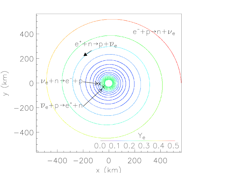
Figure 11: Electron fraction $Y_{e}$ as a function of disk position $(x,y)$ for an inspiraling mass element in the DPN disk model with $\dot{m}=1.0$, $a=0$, and $\alpha=0.1$. The markings indicate where each capture reaction becomes important, defined as where the absence of that reaction in the calculation affects $Y_{e}$ by greater than $10\%$.

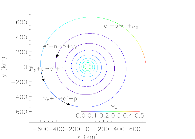
Figure 12: Same as Fig. 11 for DPN disk model $\dot{m}=10$.

The results of this section are summarized in Figs. 11 and 12. These figures show the electron fraction $Y_{e}$ as a function of position for inspiraling mass elements in the DPN disk models $\dot{m}=1$ and $10$, respectively. We note the importance of positron, neutrino, and antineutrino capture by marking the points where each interaction, when omitted, changes $Y_{e}$ by more than $10\%$.

We have calculated the fluxes coming everywhere from the surface of the disk and they affect many important pieces of physics. They alter the electron fraction in material which flows off the disk and they also determine the neutrino-antineutrino annhilation rate above the disk. A preliminary analysis of the former is in the next section. An analysis of the latter will be done in future work, but to give a point of reference: for the DPN model with $\dot{m}=1$, along the z-axis, at a height of $8\times 10^{6}{\rm cm}$ (again neglecting relativistic corrections) the neutrino number flux is $1.27\times 10^{42}{\rm cm}^{-2}$, the antineutrino number flux is $5.0\times 10^{41}{\rm cm}^{-2}$. The average energies of the neutrinos and antineutrinos at this point are 15.1 MeV and 15.7 MeV respectively, where as the rms energies are 16.4 MeV and 17.1 MeV respectively.

4 Preliminary Outflow Model

We further examine the influence of neutrinos on nucleosynthesis in GRB’s by following material from the disk as it is ejected in a wind. Neutrinos leaving the disk will interact with the outflow material, thus changing its electron fraction. Our goal here is not to develop a realistic outflow model but to estimate the import of neutrino interactions on nucleosynthesis in the wind. To this end we choose a simple constant velocity, adiabatic outflow. We assume a constant mass outflow rate proportional to $4\pi r^{2}\rho v$, which gives $\rho\sim r^{-2}$, where $r$ here is the outflow radius in the spherical approximation. The temperature in the ejecta is found from the density and the entropy per baryon. Here we assume a constant entropy per baryon in the outflow. The entropy per baryon includes the contributions from relativistic particles and nucleons, as in Qian and Woosley (1996):

$$s/k_{b}\approx 0.052\frac{T_{\mathrm{MeV}}^{3}}{\rho_{10}}+7.4+\ln\left(\frac{T_{\mathrm{MeV}}^{3/2}}{\rho_{10}}\right),$$ (26)

where $T_{\mathrm{MeV}}$ is the temperature in MeV and $\rho_{10}$ is the density in units of $10^{10}$ g/cm³. We start with a mass element in the disk, launch it with velocity $v$ equal to the escape velocity, and follow the evolution of the electron fraction in the ejecta as described in section 2.1 until the temperature drops to $10^{10}$ K.

An important difference between this calculation and that of section 2.1 is the evaluation of the effective neutrino and antineutrino fluxes at each point. We simplify the evaluation of the effective fluxes for points above the disk by assuming that the disk is essentially flat as viewed from above. Therefore each disk zone is no longer a cylindrical shell but a flat ring with radius $r_{j}$ and width $dr_{j}$. The emitted fluxes from each region first need to be adjusted for this change in geometry. Instead of multiplying the number of neutrinos emitted per second per keV per volume ($\sigma_{e}cf_{e}$ from Eqn. 13) by the width $dr_{j}$ of the zone for a cylindrical emitting surface, we multiply this quantity by the depth $d_{j}$ of the emitting zone. For the totally optically thin regions, the depth is just the total height of the disk, $d_{j}=2H$. For zones where the neutrino mean free path $l_{\nu}$ is less than $2H$, we have $d_{j}=l_{\nu}$. The height correction $h_{j}$ discussed in section 2.1 is also applicable here. The emitted neutrino flux $\phi_{\nu,j}^{\prime}$ from each zone $j$ is therefore

$$\phi_{\nu,j}^{\prime}(E_{\nu})=\phi_{\nu,j}(E_{\nu})\times h_{j}\frac{d_{j}}{dr_{j}}.$$ (27)

An equivalent expression holds for the antineutrinos.

The emitted fluxes from the optically thick region are found using the ‘neutrinosurfaces’ calculated as described in section 2.3. At each radius within the optically thick region, the emitted fluxes are calculated from Fermi-Dirac distributions according to Eqn. 19. The temperature in this expression is taken to be equal to the vertical disk temperature at the appropriate decoupling height $h_{\nu}$ or $h_{\bar{\nu}}$ for that radius, and the chemical potential is equal to $\mu_{\nu}$ or $\mu_{\bar{\nu}}$ at that disk radius. These temperatures vary along the ’neutrinosurface’. For example for DPN $\dot{m}=10$, $2.4\lesssim T_{\nu}\lesssim 6.0$ and $3.6\lesssim T_{\bar{\nu}}\lesssim 6.8$, while for DPN $\dot{m}=1$, $4.5\lesssim T_{\nu}\lesssim 5.3$ and $5.1\lesssim T_{\bar{\nu}}\lesssim 5.4$.

The effective fluxes are found by integrating the emitted fluxes over the entire disk, similar to in section 2.1 but with very different geometry. Here the appropriate solid angle is not so easily decoupled from the emitted fluxes, so we evaluate the full integral for the effective flux $\phi_{\nu}^{\prime\mathrm{eff}}$ at each point $(x,y,z)$ in the outflow,

$$\phi_{\nu}^{\prime\mathrm{eff}}(E_{\nu})=\int_{0}^{2\pi}\int_{0}^{\theta_{\mathrm{max}}(\phi)}\phi_{\nu}^{\prime}(E_{\nu},\theta,\phi)\frac{\sin\theta d\theta d\phi}{4\pi}.$$ (28)

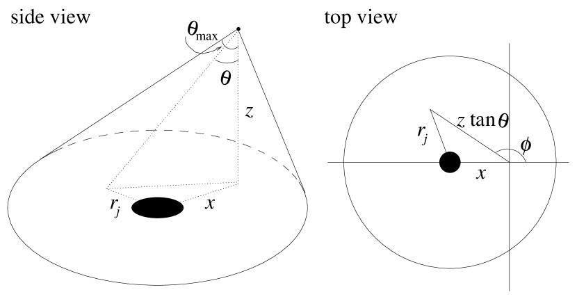
Figure 13: Illustration of the angular geometry relevant to calculating the effective neutrino flux for a point $(x,y,z)$ above the disk.

In the above expression, $\phi_{\nu}^{\prime}(E_{\nu},\theta,\phi)$ is the emitted flux $\phi_{\nu,j}^{\prime}$ at $r_{j}=[z^{2}\tan^{2}\theta+x^{2}+2xz\tan\theta\cos\phi]^{1/2}$, and $\theta_{\mathrm{max}}(\phi)$ is the maximum value for $\theta$ at the disk edge. This angular geometry is illustrated in Fig. 13.

Fig. 14 shows the minimum variation in $Y_{e}$ for two such calculations for outflows from the DPN $\dot{m}=10$ disk model. The solid line is for an outflow from close to the black hole, at $r_{\mathrm{disk}}\sim 35$ km. The short-dashed line is the equilibrium $Y_{e}$ for the same outflow. Electron capture and antineutrino capture here combine to lower $Y_{e}$ from its initial value in the disk. As the electron capture rate drops, the equilibrium $Y_{e}$ (meaning that $Y_{e}$ that would obtain if the weak rates were in equilibrium) is increasingly set by neutrino and antineutrino capture. However, $Y_{e}$ itself levels off before then since the very rapid outflow velocity ($v=v_{\mathrm{esc}}=1.5\times 10^{10}$ cm/s) causes $Y_{e}$ to quickly fall out of equilibrium. The second outflow example, the long-dashed line in Fig. 14, starts from the disk region just outside of the optically thick zone and immediately falls out of equilibrium. Here the reason is not so much that the outflow velocity is high, but that the equilibrium $Y_{e}$ rises sharply above the disk. This is entirely a neutrino-driven effect. Within the disk, the neutrino and antineutrino fluxes are quickly diminished by extinction and, most importantly, the geometric effect, so the equilibrium $Y_{e}$ is set largely by electron and positron capture. Above the disk, however, the outflow material is exposed to the high neutrino and antineutrino fluxes leaving the disk, and so the jump in the neutrino and antineutrino capture rates readjusts the equilibrium $Y_{e}$, here to a much higher value. In this example, the temperature falls below $10^{10}$ K before $Y_{e}$ levels off, but still the outflow velocity is too great (here $v=v_{\mathrm{esc}}=5.7\times 10^{9}$ cm/s) for equilibrium to be established.

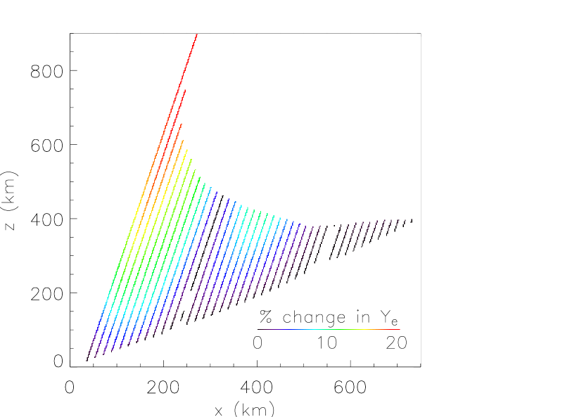
Figure 15: Percent change in $Y_{e}$, $(Y_{e}^{\mathrm{with}\;\nu}-Y_{e}^{\mathrm{no}\;\nu})\times 100/Y_{e}^{\mathrm{no}\;\nu}$, is plotted for outflows from DPN disk model $\dot{m}=10$. $Y_{e}^{\mathrm{with}\;\nu}$ includes the effects of neutrino interactions, while $Y_{e}^{\mathrm{no}\;\nu}$ is calculated with the neutrino and antineutrino capture rates set to zero.

Figs. 15 and 16 further illustrate the importance of neutrino capture in the wind. Fig. 15 compares the outflow $Y_{e}$ calculated as above to that calculated without including neutrino and antineutrino captures. The percent change in $Y_{e}$, $(Y_{e}^{\mathrm{with}\;\nu}-Y_{e}^{\mathrm{no}\;\nu})\times 100\%/Y_{e}^{\mathrm{no}\;\nu}$, is plotted for outflows from every ten radial zones in the DPN disk model with $\dot{m}=10$. In outflows from the outer disk, the neutrino flux is small and so is the percent change in $Y_{e}$. Above the inner disk, particularly above the optically thick region, the neutrino flux is much higher and $Y_{e}$ is influenced accordingly. The reason the neutrinos can have such a large influence is shown in Fig. 16. It plots the capture rates in two outflow models, (a) DPN $\dot{m}=10$ and (b) PWF $\dot{m}=0.1$, $a=0.95$, as a function of height. In both cases, the electron and positron capture rates fall quickly, dropping below the neutrino and antineutrino rates within a few hundred kilometers. The neutrino rates drop much more slowly due to the geometry of the disk. If the disk emitted neutrinos uniformly and the outflow remained above the disk, the rates would be almost constant. In our physical disks, this doesn’t hold exactly since most of the neutrinos are from the inner regions of the disk, but still the rates fall much more slowly than, for example, $\sim r^{-2}$ as in the proto-neutron star case.

It is important to note that our outflow model only conservatively estimates the influence of neutrino interactions in the wind. For example, if the velocity of the outflow is at any point slower than the escape velocity at the starting point of the flow, the wind’s exposure to the neutrino flux will be correspondingly greater. In addition, we only follow the outflow until the temperature drops below $10^{10}$ K; we expect neutrino interactions to continue to play an important role in the subsequent nucleosynthesis. This is true even for disks that are almost entirely optically thin (see, for example, Fig. 16b).

5 Conclusions

Here we have made a detailed analysis of the importance of the weak rates in the disks of gamma ray bursts. We follow mass elements as they spiral into the center of these disks, keeping track of all the rates, the emitted neutrino and antineutrino fluxes, and the electron fraction. We have included not only the effect of electron and positron capture but also of neutrino and antineutrino capture. Neutrino and antineutrino capture play an essential role for models with high accretion rates, where the neutrinos become trapped. Here the electron fraction can change by factors of several over calculations where these rates are not included. In addition, neutrinos also play an important role in models with lower accretion rates if they have high black hole spin parameter.

Even if the weak rates come into equilibrium toward the center of the disk, it is still necessary to follow the complete evolution of the mass element as we have done. This is because the lepton number of the material as it falls into the optically thick regions goes into determining the electron fraction and fluxes of neutrinos in these areas.

As part of this study, we have calculated the ’neutrinosurfaces’ or surfaces that define the regions that are optically think to neutrinos. We find that these are not spheres as in the protoneutron star case, but take on different shapes, usually more wedgelike.

As part of the larger picture, we wish to determine the nucleosynthesis that will come from the mass outflow from these disks. This will involve a hydrodynamic calculation, in addition to simply knowing the $Y_{e}$ on the disk which we have calculated here. However, whatever this outflow looks like, it is certain that the neutrino and antineutrino flux from the disk will hit it from behind as it moves out. This will change the electron fraction and therefore also any calculation of nucleosynthesis. We have made an estimate of the minimum influence of this effect by using a constant velocity for the outflowing material which is equal to the escape velocity. Even in this case, the neutrinos change the $Y_{e}$ in the outflow by 10%-60%.

Future studies of nucleosynthesis from these disks will produce exciting results. Whatever the results will be, it is certain that the neutrino interactions will have to be included in the calculations.

Appendix A Appendix

Here we describe the evaluation of the integral over the solid angle $\int d\Omega_{i,j}$ from Eqn. 18, where $d\Omega_{i,j}$ is the solid angle subtended by zone $j$ as viewed from zone $i$ within the disk. As depicted in Fig. 2, we take zone $j$ to be a uniform cylindrical shell with radius $r_{j}$, height $2H_{j}$, and thickness $dr_{j}$ and the viewpoint in zone $i$ to be a point at the midplane of the disk a distance $r_{i}$ from the black hole. The general form of the integral is as follows:

$$\int d\Omega_{i,j}=\int^{\phi_{b}}_{\phi_{a}}\int^{\theta_{b}(\phi)}_{\theta_{a}(\phi)}\sin\theta d\theta d\phi.$$ (A1)

The solid angle geometry is dependent upon whether zone $j$ is interior or exterior to zone $i$, and so the limits of integration for each case are treated separately below. Once the limits are determined we solve the integrals in Eqn. A1 numerically using the extended Simpson’s rule.

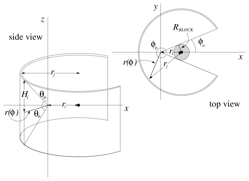
Figure 17: More detailed illustration of the solid angle, $d\Omega_{i,j}$, subtended by zone $j$ where $j$ is exterior to $i$, i.e. $r_{j}>r_{i}$.

The case where zone $j$ is exterior to zone $i$ is pictured in more detail in Fig. 17. For convenience we arrange the coordinate axes as shown, with the origin at the viewpoint in zone $i$, the $+x$ axis running along the midplane of the disk and through the black hole, and the $z$ axis extending vertically above and below the disk. In every case where $r_{j}>r_{i}$, part of zone $j$ is blocked by the event horizon and possibly an optically thick region, as depicted in the top view detail of Fig. 17. Therefore the limits of the integral over the $\phi$ coordinate become

$$\phi_{a} = \sin^{-1}\left(\frac{R_{BLOCK}}{r_{i}}\right)$$ (A2)

$$\phi_{b} = 2\pi-\sin^{-1}\left(\frac{R_{BLOCK}}{r_{i}}\right),$$ (A3)

where $R_{BLOCK}$ is the Schwarzschild radius or, if present, the radius of the optically thick region.

The limits of the integral over $\theta$, as illustrated in the side view detail of Fig. 17, are

$$\theta_{a}(\phi) = \tan^{-1}\left(\frac{r(\phi)}{H_{j}}\right)$$ (A4)

$$\theta_{b}(\phi) = \pi-\theta_{a}(\phi),$$ (A5)

where $r(\phi)$ is the distance from the origin to the midplane of zone $j$ as a function of $\phi$. The distance $r(\phi)$ is found from the law of cosines

$$r_{j}^{2}=r_{i}^{2}+r^{2}-2r_{i}r\cos\phi$$ (A6)

to be

$$r(\phi)=r_{i}\cos\phi+(r_{j}^{2}-r_{i}^{2}\sin^{2}\phi)^{1/2}.$$ (A7)

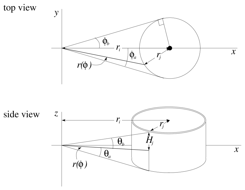
Figure 18: More detailed illustration of the solid angle, $d\Omega_{i,j}$, subtended by zone $j$ as viewed from zone $i$, for where $j$ is interior to $i$, i.e. $r_{j}<r_{i}$.

The case where zone $j$ is interior to zone $i$ is illustrated in Fig. 18. The limits of the $\phi$ integral, as shown in the top view detail, are

$$\phi_{a} = -\sin^{-1}\left(\frac{r_{j}}{r_{i}}\right)$$ (A8)

$$\phi_{b} = +\sin^{-1}\left(\frac{r_{j}}{r_{i}}\right).$$ (A9)

The side view detail of Fig. 18 shows the limits of the integral over $\theta$. The expressions for $\theta_{a}(\phi)$ and $\theta_{b}(\phi)$ are identical to Eqns. A4 and A5, except here the distance $r(\phi)$ is the negative solution of Eqn. A6,

$$r(\phi)=r_{i}\cos\phi-(r_{j}^{2}-r_{i}^{2}\sin^{2}\phi)^{1/2}.$$ (A10)

Table 1: The Electron Fraction $Y_{e}$ near the Event Horizon

Model	$\dot{m}$	$a$	$\alpha$	final $Y_{e}$
PWF	0.1	0	0.1	0.45
PWF	0.1	0	0.01	0.05
PWF	0.1	0.5	0.1	0.44
PWF	0.1	0.95	0.1	0.14
PWF	1.0	0	0.1	0.12
DPN	1.0	0	0.1	0.24
DPN	10	0	0.1	0.28

Figure 1: Disk profile for the DPN $\dot{m}=10$ disk model. The scale height $H$ of the disk is plotted versus disk radius $r$, from the Schwarzschild radius to where the temperature drops below $10^{10}$ K. The vertical long-dashed line marks the radius where the neutrino optical depth $\tau_{\nu}$ drops below 2/3, and the short-dashed line marks the equivalent point for the antineutrinos.

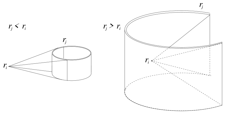
Figure 2: Illustration of the solid angle, $d\Omega_{i,j}$, subtended by zone $j$ as viewed from zone $i$, for where $j$ is interior to $i$, i.e. $r_{j}<r_{i}$, and where $j$ is exterior to $i$, i.e. $r_{j}>r_{i}$. Note that for $r_{j}>r_{i}$, part of zone $j$ is blocked by the black hole and (possibly) the optically thick region. We calculate the flux at the point $r_{i}$ from every accessible place on the surface at $r_{j}$.

Figure 3: Decoupling heights $h_{\nu}$ for neutrinos (long dashes) and antineutrinos (short dashes) versus radius in the DPN disk model $\dot{m}=1.0$. The solid line marks the scale height $H$ of the disk.

Figure 4: Same as Fig. 3 for the DPN disk model $\dot{m}=10$.

Figure 5: Electron fraction $Y_{e}$ as a function of radius for the PWF models with $\dot{m}=0.1$, alpha viscosity $\alpha=0.1$, and black hole spin parameter $a=0$. The solid line shows $Y_{e}$ from our full calculation, while the dotted line is our calculation without neutrino interactions. The dashed line is the $Y_{e}$ that would obtain, were the system in weak equilibrium.

Figure 6: Identical to Fig. 5 for the PWF disk model with $\dot{m}=0.1$, $\alpha=0.1$, and $a=0.95$. Again the solid line is the full calculation and the dotted is the calculation without neutrinos. The rise at the center of the disk is due to neutrino trapping. The additional dot-dashed line shows our calculation with just the antineutrinos turned off.

Figure 7: Effective neutrino fluxes from the optically thick region divided by the net flux emitted by the optically thick region, for the PWF disk model with $\dot{m}=0.1$, $\alpha=0.1$, and $a=0.95$. The dot-dashed line is for the antineutrino flux and the solid and dotted lines are for the neutrino flux calculated with and without the extinction correction, respectively. The dashed line shows $r^{-2}$ for comparison.

Figure 8: Electron fraction $Y_{e}$ as a function of radius for the DPN and PWF disk models with $\dot{m}=1$, black hole spin parameter $a=0$, and alpha viscosity $\alpha=0.1$. The dot-dashed line shows $Y_{e}$ calculated with the PWF disk model, while the remaining three lines are from the DPN disk model. The solid line shows $Y_{e}$ from our full calculation, the dotted line is for a calculation without neutrino interactions, and the dashed line shows the equilibrium $Y_{e}$.

Figure 9: Net neutrino fluxes versus radius for the DPN disk models with (a) $\dot{m}=1$ and (b) $\dot{m}=10$. The dark solid (dashed) lines show the net effective (anti)neutrino flux at each radius, while the lighter weight lines show the net neutrino flux emitted from each optically thin zone. The filled and unfilled circles depict the net antineutrino and neutrino fluxes, respectively, from the optically thick region and are plotted at the effective ‘neutrinosurface’ radii $r_{\nu}$.

Figure 10: Electron fraction $Y_{e}$ as a function of radius for the DPN disk model with $\dot{m}=10$, $a=0$, and $\alpha=0.1$. As in Fig. 8, the solid line is the full calculation with neutrino interactions, the dotted line without, and the dashed line shows the equilibrium $Y_{e}$.

Figure 14: Electron fraction versus height in the outflow originating from two locations within the DPN disk model $\dot{m}=10$: close to the black hole ($r\sim 35$ km, solid line) and at the outer edge of the optically thick region ($r\sim 250$ km, long-dashed line). The short-dashed line and dotted line show the equilibrium $Y_{e}$ for each outflow.

Figure 16: Capture rates versus height in the outflow originating from two disk models, (a) DPN $\dot{m}=10$ and (b) PWF $\dot{m}=0.1$, $a=0.95$. For both models, the solid line is the electron capture rate, the long-dashed line is the positron capture rate, the short-dashed line is the antineutrino capture rate, and the dotted line is the neutrino capture rate. As shown, the neutrino and antineutrino capture rates remain high well above the disk.

References

- Beloborodov (2003) Beloborodov, A. M. 2003, ApJ, 588, 931
- DiMatteo, Perna, and Narayan (2002) DiMatteo, T., Perna, R., and Narayan, R. 2002 ApJ, 579, 706.
- Eichler et al. (1989) Eichler, D., Livio, M., Piran, T., and Schramm, D. N. 1989, Nature, 340, 126.
- Fryer et al. (1999) Fryer, C. L., Woosley, S. E., Herant, M., and Davies, M. B. 1999, ApJ, 526, 152.
- Lattimer and Swesty (1991) Lattimer, J. M. and Swesty, F. D. 1991, Nucl. Phys. A, 535, 331.
- MacFadyen and Woosley (1999) MacFadyen, A. I. and Woosley, S. E. 1999, ApJ, 524, 262.
- MacFadyen, Woosley, and Heger (2001) MacFadyen, A. I., Woosley, S. E. and Heger, A. 2001, ApJ, 550, 410.
- Mészáros (2002) Mészáros, P. 2002, ARA&A, 40, 137.
- Narayan, Paczyński, and Piran (1992) Narayan, R., Paczyński, B., and Piran, T. 1992, ApJ, 395, L83.
- Narayan, Piran, and Kumar (2001) Narayan, R., Piran, T., and Kumar, P. 2001, ApJ, 557, 949.
- Paczyński (1991) Paczyński, B. 1991, Acta Astron., 41, 157.
- Paczyński (1998) Paczyński, B. 1998, ApJ, 494, L45.
- Popham, Woosley, and Fryer (1999) Popham, R., Woosley, S. E., and Fryer, C. 1999, ApJ, 518, 356.
- Pruet, Fuller, & Cardall (2001) Pruet, J., Fuller, G. M., & Cardall, C. Y. 2001, ApJ, 561, 957
- Pruet, Woosley, and Hoffman (2002) Pruet, J., Woosley, S. E., and Hoffman, R. D. 2003, ApJ, 586, 1254.
- Qian and Woosley (1996) Qian, Y.-Z., and Woosley, S. E. 1996, ApJ, 471, 331.
- Ruffert and Janka (1999) Ruffert, M., and Janka, H.-T., 1999, A&A, 344, 573.
- Ruffert and Janka (2001) Ruffert, M., and Janka, H.-T., 2001, A&A, 380, 544.
- Vietri and Stella (1998) Vietri, M. and Stella, L. 1998, ApJ, 507, L45.
- Woosley (1993) Woosley, S. E. 1993, ApJ, 405, 273.