Pixel correlation searches for O VI in the Lyman $\alpha$ forest and the volume filling factor of metals in the Intergalactic Medium at $z\sim 2-3.5$

Abstract

Artificial absorption spectra are used to test a variety of instrumental and physical effects on the the pixel correlation technique for the detection of weak O vi absorption. At H i optical depths $\raisebox{-2.58334pt}{$\,\stackrel{{\scriptstyle\raisebox{-0.60275pt}{$\textstyle<$}}}{{\sim}}\,$}0.3-1$, the apparent O vi detections are spurious coincidences due to H i absorption at other redshifts. In this range, the apparent O vi optical depth is independent of H i optical depth. At larger H i optical depths, apparent O vi optical depth and H i optical depth are correlated. Detailed modelling is required in order to interpret the significance of this relation. High-resolution spectra of four QSOs together with a large suit of synthetic spectra are used to show that the detection of O vi in individual spectra is only statistically significant for overdensities $\raisebox{-2.58334pt}{$\,\stackrel{{\scriptstyle\raisebox{-0.60275pt}{$\textstyle>$}}}{{\sim}}\,$}5$. These overdensities are larger than would be naively inferred from the onset of the correlation and a tight optical depth-density relation. The lower limit for the volume filling factor of regions which are enriched by O vi is 4% at 95% confidence. This is no larger than the observed volume filling factor of the winds from Lyman break galaxies. Previous claims that the observed O vi absorption extends to underdense regions and requires a universal metal enrichment with large volume filling factor, as may be expected from population III star formation at very high redshift, appear not to be warranted.

1 Introduction

The Ly$\alpha$ forest in QSO absorption spectra is now widely believed to be caused by fluctuating Gunn-Peterson absorption due to an undulating warm photoionised Intergalactic Medium (IGM). With this interpretation for the origin of the Ly$\alpha$ forest, it has become possible to relate the absorption optical depth to the density of absorption systems in a meaningful manner. According to this scheme low column density absorption systems arise from low density regions of the Universe. A detection of associated metal absorption in weak Ly$\alpha$ absorption systems would suggest that the metal enrichment of the IGM is widespread.

Models put forward to explain this metal enrichment fall into two categories: they either propose that early and widespread Population III star formation in pre-galactic structures at $z\raisebox{-2.58334pt}{$\,\stackrel{{\scriptstyle\raisebox{-0.60275pt}{$\textstyle>$}}}{{\sim}}\,$}10$ is responsible (e.g. Nath & Trentham 1997; Ferrara, Pettini & Shchekinov 2000; Barkana & Loeb 2001; Madau, Ferrara & Rees 2001) or suggest a later episode of metal enrichment by winds from starbursting galaxies at $z\leq 5$ (e.g. Aguirre et al. 2001, Theuns et al. 2001, Adelberger et al. 2003). Transporting metals from the galaxies or protogalaxies where they are produced into the (low density) IGM is not, however, a trivial matter. A variety of mechanisms have been proposed. Some have argued for supernova-driven (Couchman & Rees 1986, Dekel & Silk 1986) or ‘miniquasar’-driven (Haiman, Madau & Loeb, 1999) winds. Others have argued for ejection via galactic mergers (Gnedin & Ostriker 1997 and Gnedin 1998) or photoevaporation during reionisation (Barkana & Loeb, 1999). With an accurate determination of the fraction of the universe (or ‘volume filling factor’) enriched by metals it may be possible to test the veracity of such models. A large volume filling factor would favour early enrichment by stars forming in shallow potential wells, out of which metals are more easily transported into low density regions.

Observationally, the most important tracers of metals in the photoionised IGM are C iv and O vi . Associated C iv absorption has been detected down to HI column densities of order $10^{14}{\,{\rm cm}}^{-2}$ (Tytler et al. 1995, Cowie et al. 1995, Ellison et al. 2000, Pettini et al. 2003) corresponding to an optical depth of $1-10$. To investigate even lower density systems a pixel correlation technique has been employed where, instead of fitting an associated C iv absorption line, a pixel-by-pixel search for excess absorption at the corresponding C iv wavelength is performed (Cowie & Songaila, 1998). This method was hoped to be more robust than the use of line ‘stacking’ (Tytler et al. 1995; Ellison et al. 2000), but there is some ambiguity in the interpretation of the results. At the relevant redshifts, the O vi species is the most sensitive tracer of metals in low density regions of the IGM, provided that the spectrum of the UV background is sufficiently hard (Rauch, Haehnelt & Steinmetz 1997 and Hellsten et al. 1998). However, the relevant O vi absorption lines ($\lambda_{O\textsc{vi}a}=1032$Å, $\lambda_{O\textsc{vi}b}=1038$Å) occur in the same wavelength range as the Lyman $\alpha$ forest and higher order lines of the Lyman series, which makes the detection of weak O vi absorption challenging.

Schaye et al. (2000) claim to have detected O vi at H i optical depths significantly smaller than unity in some QSO absorption spectra and used the optical depth-density relation of numerical hydrodynamic simulations to argue that this indicates a detection of metals in underdense regions of the IGM. In this work, we apply the pixel-by-pixel search to synthetic spectra and thereby investigate instrumental and physical effects on this technique (see also Aguirre, Schaye & Theuns 2002). We then assess the statistical significance of the O vi detection and the implied density threshold above which the presence of metals is confidently detected.

The spectra (both simulated and observed) are described in Section 2. In Section 3 we outline the pixel correlation method used to detect the presence of O vi absorption. The results of the search for O vi are shown and discussed in Section 4. In Section 5 we explore the consequences for the metal enrichment of the low density IGM.

2 Simulated and Observed Spectra

2.1 Calculating synthetic spectra

2.1.1 Basic Assumptions

We use the method developed by Bi (Bi, Boerner & Chu 1992; Bi & Davidsen 1997) to analytically calculate synthetic spectra in the fluctuating Gunn-Peterson approximation for a warm photoionised IGM with a density distribution that is expected in a $\Lambda$CDM structure formation model. The basic assumptions are:

1. the baryonic matter traces the dark matter on scales larger than a filtering scale, which is related to the Jeans scale;

2. the distribution of mildly non-linear densities has a lognormal probability distribution function (PDF);

3. the absorbing gas obeys a simple temperature-density relation and is not shock-heated.

Table 1 shows the model parameters. A brief summary of how we calculate the synthetic spectra follows.

Table 1: Model parameters used for all simulations

Parameter	Chosen Value
$\Omega_{\rm m}$	0.3
$h$	0.65
$\Omega_{\lambda}$	0.7
$\sigma_{\rm 8}$	0.9
$log[\bar{T}_{\rm{eff}}]$	4.6
$\mu$	0.641
$\Gamma$	1.333

2.1.2 The Spatial Distribution of Baryons

According to standard structure formation models the matter distribution was initially a Gaussian random field with small density fluctuations that evolve under gravity into the pattern of sheets and filaments characteristic of CDM models. Many features of such a distribution can be reproduced by a rank-ordered mapping of a linear Gaussian random field onto a lognormal PDF of the density. This idea is at the heart of the method used to calculate synthetic absorption spectra (Bi et al., 1992). This method is an efficient way of producing large numbers of realistic synthetic spectra. Note that we are interested in producing synthetic spectra with a realistic density PDF and realistic instrumental properties. Reproducing the detailed clustering properties of the density field is less important.

We begin by creating a linear Gaussian random field which is fully determined by its power spectrum, $P_{DM}(k)$, for which we have used the form given by Efstathiou, Bond & White (1992),

$$P_{\rm DM}(k)\propto\frac{k}{(1+[ak+(bk)^{3/2}+(ck)^{2}]^{\nu})^{2/\nu}},$$ (1)

where $a=6.4/\Gamma$, $b=3.0/\Gamma$, $c=1.7/\Gamma$, $\Gamma=\Omega_{m}h$ ($\Omega_{m}$ & $h$ have their normal definitions) and $\nu=1.13$. The power spectrum was normalised by the rms fluctuation amplitude on a $\mathrm{8h^{-1}Mpc}$ scale, $\sigma_{8}$, as given in Table 1. In order to take into account pressure effects that suppress fluctuations on scales smaller than a certain filtering scale (Gnedin & Hui, 1998) the power spectrum of the baryon density in the linear regime is assumed to have the form,

$$P_{\rm B}(k)=\frac{P_{\rm{DM}}(k)}{(1+x_{\rm b}^{2}k^{2})^{2}},\qquad x_{\mathrm{b}}=\left[\frac{2\gamma k\bar{T}_{\rm{eff}}}{3\mu m_{\rm p}\Omega(1+z)}\right]^{\frac{1}{2}},$$ (2)

where $x_{\mathrm{b}}$ is a comoving scale related to the Jeans length (Peebles 1980; Bi & Davidsen 1997), $\gamma$ is the ratio of specific heats, $\bar{T}_{\rm{eff}}$ is the effective mean temperature and $\mu$ is the molecular weight of the IGM. An appropriate value for $\bar{T}_{\rm{eff}}$ has been determined from comparison with hydrodynamic simulations by Bi & Davidsen (1997). This is the baryonic matter power spectrum at $z=0$ and linear theory is used to evolve it backward to high redshift.

Equations (1) and (2) provide the 3D power spectrum. A 1D power spectrum needed for the description of line-of-sight (LOS) fluctuations is obtained by an integration of the 3D power spectrum (Kaiser & Peacock, 1991). The matter density and the peculiar velocity field are related and can be described as coupled Gaussian random fields (see Bi et al. 1992 for more details). Random realisations of the density and peculiar velocity in real space (co-moving coordinates) are obtained using a Fourier transform routine. The non-linear evolution is modelled by a local rank-ordered mapping to a lognormal density probability distribution,

$$n/\bar{n}=\exp\left[\delta(x)-\frac{\langle\delta^{2}\rangle}{2}\right].$$ (3)

where $\delta=(n-\bar{n})/\bar{n}$ and $n/\bar{n}$ is the overdensity factor. At the relevant redshift the baryonic density field is still in the mildly non-linear regime and the use of a log-normal PDF is a reasonable assumption (Bi et al. 1992; Nusser & Haehnelt 2000).

2.1.3 From the density to the absorption spectrum

The H i optical depth depends not only on the density but also on the temperature of the gas, due to the temperature dependence of the recombination rate. For densities $n/\bar{n}\raisebox{-2.58334pt}{$\,\stackrel{{\scriptstyle\raisebox{-0.60275pt}{$\textstyle<$}}}{{\sim}}\,$}10$, numerical simulations show that most of the gas is not shocked and that a simple power law relation between density and temperature is established by the balance of photoionisation heating and adiabatic cooling (Hui & Gnedin, 1997),

$$T=T_{0}(n/\bar{n})^{\alpha},$$ (4)

where $0.3\raisebox{-2.58334pt}{$\,\stackrel{{\scriptstyle\raisebox{-0.60275pt}{$\textstyle<$}}}{{\sim}}\,$}\alpha\raisebox{-2.58334pt}{$\,\stackrel{{\scriptstyle\raisebox{-0.60275pt}{$\textstyle<$}}}{{\sim}}\,$}0.6$ and $T_{0}$ is a constant.

For gas at temperatures of a few times $10^{4}K$ in photoionisation equilibrium the neutral hydrogen density is proportional to $n^{2}T^{-0.7}/\Gamma_{\mbox{H\,{\sc i}}}$, where $\Gamma_{\mbox{H\,{\sc i} }}$ is the photoionisation rate. As a result, the optical depth to Ly$\alpha$ absorption at redshift $z$ can be written as

Table 2: Observed Data Sample

QSO	$\mathrm{z_{em}}$	$\mathrm{z_{range}}$	$\mathrm{\bar{D}_{\textsc{ovi}}}$	$\mathrm{\bar{D}_{\textsc{hi}}}$
Q1122-165	2.40	2.02-2.34	0.157	0.165
Q1442+293	2.67	2.51-2.63	0.194	0.193
Q1107+485	3.00	2.71-2.95	0.254	0.253
Q1422+231	3.62	3.22-3.53	0.418	0.386

$$\tau_{\mathrm{Ly}\alpha}(z)=\sigma_{0}\bar{n}_{\rm HI}I(z),$$ (5)

where

$$I(z)=\int_{z_{1}}^{z_{2}}\frac{cdz^{\prime}}{1+z}\frac{c}{H_{0}E(z^{\prime})}\left(\frac{n(z^{\prime})}{\bar{n}}\right)^{1.7}$$ (6)

$${}\frac{1}{b}\exp\left(-\left(\frac{c(z-z^{\prime})}{(1+z)}+v_{\rm pec}(z^{\prime})\right)^{2}\Bigg{/}b^{2}\right),$$

$z_{1}$ and $z_{2}$ are the lower and upper limits of the redshift region of interest, $b$ is the Doppler parameter, $n_{\rm HI}$ is the neutral hydrogen density, $v_{\rm pec}$ is the peculiar velocity and a value $\alpha=0.4$ is assumed. $E(z)$ is the redshift dependent component of the Hubble parameter and $\sigma_{0}$ is the cross-section for resonant Ly$\alpha$ scattering.

The effect of peculiar velocity and Doppler broadening are taken into account to obtain the optical depth in redshift space. We have thereby approximated the Voigt profile by a Gaussian distribution, which is a reasonable approximation for absorption lines with equivalent width $<0.7$Å.

The optical depth for the O vi doublet is calculated assuming a fixed ratio of O vi number density to H i number density ($n_{\mathrm{O\textsc{VI}}}/n_{\mathrm{H\textsc{I}}}$). The optical depth of the higher order Lyman lines are also calculated.

2.1.4 Realistic Synthetic Spectra

To facilitate a more accurate comparison with the observed spectra we model the optical depth distribution for the same wavelength range as the observed spectra. There are two regions of the spectra of particular interest; the ‘O vi region’, where O vi absorption is searched for, and the ‘H i region’, where the corresponding Ly$\alpha$ absorption occurs. The spectra are obtained by co-adding the optical depth of Ly$\alpha$, O vi and higher order Lyman series lines. We then use the estimated statistical error on the flux for the observed spectrum to add random noise and perform a Gaussian smoothing to mimic the effect of instrumental broadening.

The optical depth is scaled such that the mean flux decrement of the observed QSO is reproduced. As we will discuss later the results of the pixel-by-pixel search depend sensitively on the mean flux level. We have thus rescaled the optical depth for the H i and the O vi regions independently to reproduce the observed mean flux level in both regions ($\bar{D}_{\mathrm{\textsc{hi}}}$ and $\bar{D}_{\mathrm{\textsc{ovi}}}$ respectively). $\bar{D}_{\mathrm{\textsc{hi}}}$ is used to set $\bar{\tau}_{\mathrm{Ly}\alpha}$ in the H i region as well as $\bar{\tau}_{\mathrm{O\textsc{vi}}}$ (with fixed $n_{\mathrm{O\textsc{VI}}}/n_{\mathrm{H\textsc{I}}}$) and the optical depth of the higher order Lyman lines in the O vi region. $\bar{D}_{\mathrm{O\textsc{vi}}}$ is then used to set $\bar{\tau}_{\mathrm{Ly\alpha}}$ in the O vi region. Note that this means that we allow a difference in the value of $\Omega_{\mathrm{bar}}^{2}/\Gamma_{\mathrm{H\textsc{i}}}$ in the two regions of the spectrum. It seems plausible to assume that the errors we obtain in this way for a range of Monte Carlo realisations of the LOS density distribution are similar to those we would have found if we had only picked random realisations that can reproduce the mean flux decrement in the H i and the O vi regions simultaneously. The latter approach is computationally prohibitive.

In this way we have obtained ensembles of simulated spectra with the same wavelength range, mean flux decrement and noise properties as the observed spectra, but differing in their specific random realisation of LOS matter distribution and noise.

2.2 Observations

We have used four observed QSOs which are part of the sample used by Schaye et al. (2000) for a detailed comparison with synthetic QSOs spectra: Q1122-165, Q1442+293, Q1107+485 and Q1422+231. The data for Q1122-165 was taken during Commissioning I and Science Verification observations for the UVES instrument on the VLT (Kueyen) and released by ESO for public use. The reduction method can be found in Kim, Cristiani & D’Odorico (2001). The other spectra were taken with the HIRES instrument (Vogt S. S. et al., 1994) on Keck I and reduced using procedures described in Barlow & Sargent (1997). These two instruments provide spectra with resolutions $R_{\mathrm{max}}\approx$ 80000 and 110000 respectively and have typical S/N of 50. Table 2 gives a list of the redshift range and flux decrement for the O vi and H i regions. Regions of strong absorption from other known metal lines were removed.

3 Pixel-by-pixel search

Figure 1: An example of the results from the pixel-by-pixel search method for the absorption spectrum of Q1107+485.

We use a technique for the detection of O vi in the Lyman $\alpha$ forest initially developed by Cowie & Songaila (1998) for the detection of weak C iv absorption. Schaye et al. (2000) adapted this method to search for the O vi doublet (see also Aguirre et al. 2002). We briefly summarise the procedure here. The redshift range explored in each of the four QSOs is shown in Table 2. This is the same as used by Schaye et al. (2000). Due to the increase in noise we did not find it worthwhile to extend the search to lower wavelength.

The continuum-fitted absorption spectrum is re-binned to pixels of equal size in redshift space for the Lyman series and both members of the O vi doublet. A width of $(c\Delta\lambda/\lambda_{\mathrm{Ly}n}\mathrm{)kms^{-1}}$ is taken (where Lyn is the highest order Lyman line used). In order to take into account possible velocity shifts between O vi and H i absorption, we have also tried larger pixels widths. This did not improve the sensitivity for O vi detection.

A search for correlated absorption at the wavelengths of the Lyman series and the O vi doublet is then performed. Each pixel of the Ly$\alpha$ absorption region is considered in turn. If the flux level is within $\sigma_{\mathrm{noi}}/2$ of the continuum level (where $\sigma_{\mathrm{noi}}$ is the estimated statistical error on the flux for the observed spectrum) or in a region where the associated O vi absorption is not covered the pixel is discarded. If the pixel is within $\sigma_{\mathrm{noi}}/2$ of saturation we attempt to use the higher order Lyman lines to estimate $\tau_{\rm{Ly}\alpha}$. We thereby use the higher order line with the lowest equivalent Ly$\alpha$ optical depth $\tau_{{\rm Ly}\alpha}=\min(\tau_{{\rm Ly}n}f_{{\rm Ly}\alpha}/f_{{\rm Ly}n}\lambda_{{\rm Ly}n})$ that is not within $\sigma_{\mathrm{noi}}/2$ of saturation or the continuum (where $f_{{\rm Ly}n}$ is the oscillator strength of the Lyn line).

Once we have established a value for $\tau_{\mathrm{Ly}\alpha}$, we consider the pixels corresponding to absorption by the O vi doublet at the same redshift. The limiting factor in the use of this method is coincident absorption from H i, either in the form of higher order Lyman lines at similar redshift or by Ly$\alpha$ lines at lower redshift. Obviously we want to minimise this contamination. The doublet nature of the O vi is utilised in this regard. The smaller equivalent absorption,

$$\tau_{\mathrm{O\textsc{vi}}}={\rm min}\left(\tau_{\mathrm{O\textsc{vi}a}},\frac{f_{\mathrm{O\textsc{vi}a}}\lambda_{\mathrm{O\textsc{vi}a}}\tau_{\mathrm{O\textsc{vi}b}}}{f_{\mathrm{O\textsc{vi}b}}\lambda_{\mathrm{O\textsc{vi}b}}}\right),$$ (7)

will be the least contaminated. This gives us an upper limit to the O vi optical depth. We will thus call the O vi optical depth obtained in this way the apparent O vi optical depth.

As pointed out by Aguirre et al. (2002) the contamination by higher order Lyman lines can be estimated from the corresponding Ly$\alpha$ absorption and corrected. Such contamination is subtracted from the O vi optical depth where possible. If this is not possible because of saturated Ly$\alpha$ absorption we also discard the pixel.

We then bin the ensemble of optical depth pairs in Ly$\alpha$ optical depth and plot the relation between the median optical depth of O vi and Ly$\alpha$ . We use the median instead of the mean as the distribution of O vi optical depth in each bin is skewed toward high optical depths due to the contamination by H i absorption.

Fig. 1 shows an example of the relation of the apparent O vi and Ly$\alpha$ optical depth (${\tau_{\mathrm{O\textsc{VI},app}}-\tau_{\mathrm{Ly}\alpha}}$ relation) obtained in this way. At small Ly$\alpha$ optical depth, the median O vi optical depth is constant. As we will demonstrate in detail in the next section (see also Aguirre et al. (2002)), the apparent O vi is here almost exclusively due to contamination of coincident H i absorption and this region of the diagram cannot be used to infer a detection of O vi . At larger Ly$\alpha$ optical depth, the apparent O vi optical depth rises and is mainly due to the presence of O vi . The level of metal enrichment is, however, not straightforward and requires detailed modelling.

Figure 2: A sketch showing the dependence of the ${\tau_{\mathrm{O\textsc{VI},app}}-\tau_{\mathrm{Ly}\alpha}}$ relation on the principal parameters $\bar{D}_{\mathrm{O\textsc{vi}}}$, $n_{\mathrm{O\textsc{VI}}}/n_{\mathrm{H\textsc{I}}}$ and $(n/\bar{n})_{\mathrm{cut}}$.

Figure 3: The ${\tau_{\mathrm{O\textsc{VI},app}}-\tau_{\mathrm{Ly}\alpha}}$ relation for an ensemble of forty synthetic spectra. Left: $\mathrm{\bar{D}_{O\textsc{VI}}}$ increases from bottom to top. Right: $\mathrm{\bar{D}_{H\textsc{I}}}$ increases from bottom to top

4 Results From Simulated Spectra

4.1 Principle parameters

To obtain an indication of how the pixel-by-pixel search depends upon instrumental effects and physical parameters and what errors should be expected due to variation of the LOS density distributions, we investigated a large suit of synthetic spectra. We have varied the mean flux decrement in the O vi and H i regions ($\bar{D}_{\mathrm{O\textsc{vi}}}$ and $\bar{D}_{\mathrm{H\textsc{i}}}$), the ratio of O vi to H i density ($n_{\mathrm{O\textsc{vi}}}/n_{\mathrm{H\textsc{i}}}$) and introduced a varying cut-off in the density below which we set the O vi density to zero ($(n/\bar{n})_{\mathrm{cut}}$ ). Fig. 2 sketches how the relation of apparent O vi optical depth and Ly$\alpha$ optical depth depends on the three key parameters $\bar{D}_{\mathrm{O\textsc{vi}}}$, $(n/\bar{n})_{\mathrm{cut}}$ and $n_{\mathrm{O\textsc{vi}}}/n_{\mathrm{H\textsc{i}}}$. A detailed discussion of the effect of these and the other parameters using synthetic spectra of Q1122 will follow below. The parameters were varied around fiducial values denoted by an ‘F’ in figures 3-5. The error bars in these figures are the $1\sigma$ spread of the optical depths for ensembles of 40 spectra.

4.2 Varying the mean optical depth

Fig. 3 shows how changing the mean flux decrement affects the ${\tau_{\mathrm{O\textsc{VI},app}}-\tau_{\mathrm{Ly}\alpha}}$ relation. In the left panels we consider changes in the O vi region, $\bar{D}_{\mathrm{O\textsc{vi}}}$. With increasing flux decrement the level of spurious coincidences due to Ly$\alpha$ absorption from gas at a lower redshift rises and mimics the detection of O vi . Since this Ly$\alpha$ absorption is uncorrelated with absorption in the H i region, this leads to a floor of constant apparent O vi optical depth which rises with increasing $\bar{D}_{\mathrm{O\textsc{vi}}}$. In the right panels of Fig. 3 we vary the mean flux decrement in the H i region $\bar{D}_{\mathrm{H\textsc{i}}}$. This time the shape of the relation between H i optical depth and apparent O vi optical depth does not change but the error bars increase substantially with decreasing mean flux decrement. This is because, for small mean flux decrement, large optical depth Ly$\alpha$ pixels are poorly sampled.

4.3 Varying the O vi distribution

Figure 4: As Figure 3. Left: $n_{O\textsc{vi}}/n_{H\textsc{i}}$ increases from top to bottom. Right: $(n/\bar{n})_{\mathrm{cut}}$ increases from top to bottom.

In Fig. 4 we vary the O vi distribution for our synthetic spectra. The left panels shows how varying the ratio of O vi to H i density affects the ${\tau_{\mathrm{O\textsc{VI},app}}-\tau_{\mathrm{Ly}\alpha}}$ relation. With increasing ratio a correlation between apparent O vi optical depth and H i optical depth develops for large H i optical depth but the errors are large. As discussed in the introduction the main aim of the search for O vi at small H i optical depth is to establish the volume filling factor of metals in the Universe. Because of the possible spurious detections due to random coincidences this is not straightforward.

There is another important effect which can lead to spurious detection of O vi . Low Ly$\alpha$ optical depth is not necessarily associated with low density gas but can also be due to the wing of a strong Ly$\alpha$ absorption feature which is caused by a high density region. In order to test the density range for which the presence of O vi is required to reproduce the observed ${\tau_{\mathrm{O\textsc{VI},app}}-\tau_{\mathrm{Ly}\alpha}}$ relation, we introduce a cut-off in the density, $(n/\bar{n})_{\mathrm{cut}}$ below which we set the O vi density to zero, i.e.

$$\frac{n_{OVI}}{n_{HI}}=0,\quad\textrm{if}\quad\frac{n}{\bar{n}}<\left(\frac{n}{\bar{n}}\right)_{\mathrm{cut}},$$ (8)

$$\frac{n_{OVI}}{n_{HI}}=\textrm{const},\quad\textrm{if}\quad\frac{n}{\bar{n}}\geq\left(\frac{n}{\bar{n}}\right)_{\mathrm{cut}}.$$ (9)

In the right panel of Fig. 4 we vary $(n/\bar{n})_{\mathrm{cut}}$. The onset of the correlation moves to larger H i optical depth. Unfortunately, this dependence is weak.

4.4 Varying S/N and continuum level

The left panels of Fig. 5 show the effect of changing the simulated noise. As expected, the errors increase significantly with increasing noise level.

The effect of an error in the continuum fit is shown in the right panels of Fig. 5, where we have raised and lowered the continuum as a whole by 1% in each synthetic spectrum. When we raise the continuum level the apparent O vi optical depth increases because the optical depth of spuriously coincident H i absorption increases. Note that if the continuum is placed too low the correlation between H i and O vi optical depth misleadingly appears to extend to smaller H i optical depth.

Figure 5: As Figure 3. Left: noise increases from top to bottom. Right: the continuum level increases from top to bottom.

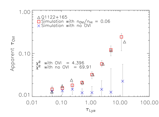
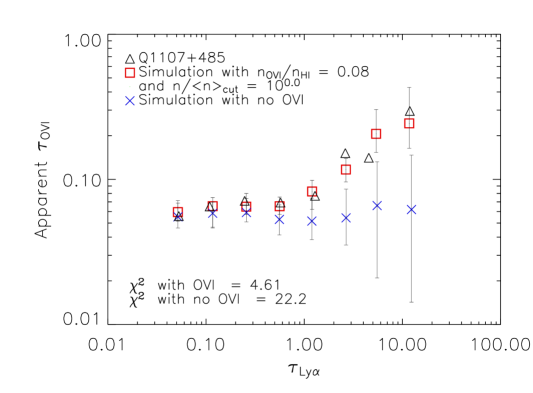
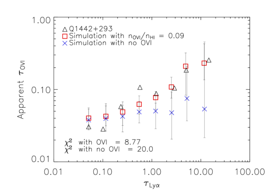
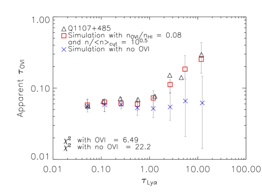
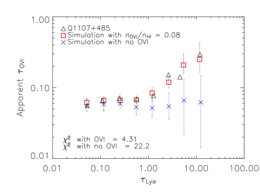
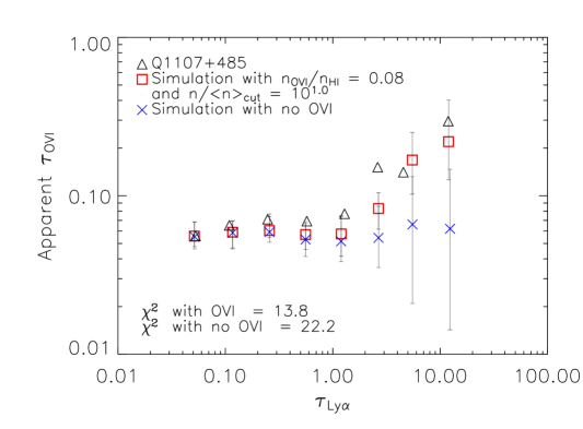
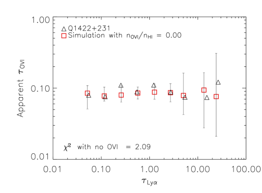
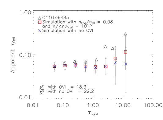
Figure 6: Right: the ${\tau_{\mathrm{O\textsc{VI},app}}-\tau_{\mathrm{Ly}\alpha}}$ relation for observed and simulated synthetic spectra for four QSOs; this is shown for synthetic spectra with both the best best fitting constant ratio of $n_{\rm{O\textsc{vi}}}/n_{\rm{H\textsc{i}}}$ and with no O vi . Left: the effect of varying $(n/\bar{n})_{\mathrm{cut}}$ on synthetic spectra of Q1107 compared to the ${\tau_{\mathrm{O\textsc{VI},app}}-\tau_{\mathrm{Ly}\alpha}}$ relation of the observed spectrum.

5 Search for O vi in the low density IGM

5.1 Comparison of real and simulated spectra

Here we perform a detailed comparison between four observed QSO spectra and sets of synthetic spectra. We use the same S/N, $\bar{D}_{\mathrm{O\textsc{VI}}}$, $\bar{D}_{\mathrm{H\textsc{I}}}$ and wavelength range as in the observed spectra with one exception. In the case of Q1122 we decrease $\bar{D}_{\mathrm{O\textsc{VI}}}$ by 35% in order to reproduce the level of apparent $\tau_{\mathrm{O\textsc{vi}}}$ at low $\tau_{\mathrm{H\textsc{i}}}$. The need for this is most likely due to a deficit of saturated regions in our synthetic spectra. The contribution of saturated regions to the mean flux decrement is high at low redshift and the failure to adequately reproduce the high incidence of these systems leads to a bias in the mean flux decrement (Viel et al., 2003).

The triangles in the left panel of Fig. 6 show the ${\tau_{\mathrm{O\textsc{VI},app}}-\tau_{\mathrm{Ly}\alpha}}$ relation for the four observed spectra. For the synthetic spectra we assume as before that the O vi distribution takes the form described in equations (8) and (9). We have varied the O vi density and the overdensity threshold for addition of O vi over the range $n_{\mathrm{O\textsc{VI}}}/n_{\mathrm{H\textsc{I}}}=0-0.3$ and $(n/\bar{n})_{\mathrm{cut}}=0-100$. We have produced samples of 40 synthetic spectra for each set of values. We have then calculated the ${\tau_{\mathrm{O\textsc{VI},app}}-\tau_{\mathrm{Ly}\alpha}}$ relation for each sample and assessed the agreement with the observed relation by calculating $\chi^{2}$. Note, however, that there may be additional sources of error such inhomogeneities in the metal distribution which our Monte Carlo technique does not take into account. The crosses and squares in the left panels of Fig. 6 show the ${\tau_{\mathrm{O\textsc{VI},app}}-\tau_{\mathrm{Ly}\alpha}}$ relation with no O vi and the best fitting values for $n_{\mathrm{O\textsc{VI}}}/n_{\mathrm{H\textsc{I}}}$ ($(n/\bar{n})_{\mathrm{cut}}$ $=0$), respectively. The best fitting value has a reduced $\chi^{2}_{\mathrm{r}}$ close to or somewhat smaller than one. There is thus good agreement between the ${\tau_{\mathrm{O\textsc{VI},app}}-\tau_{\mathrm{Ly}\alpha}}$ relation for our best fitting simulations and the real data. In the right panels of Fig. 6 we use the ${\tau_{\mathrm{O\textsc{VI},app}}-\tau_{\mathrm{Ly}\alpha}}$ relation of synthetic and observed spectra for Q1107 to provide an example of the difficulty in constraining $(n/\bar{n})_{\mathrm{cut}}$ .

The top panel of Fig. 7 shows the reduced $\chi^{2}_{\mathrm{r}}$ as a function of $n_{\mathrm{O\textsc{VI}}}/n_{\mathrm{H\textsc{I}}}$ for the four observed QSOs. In Q1442 there is a marginal detection of O vi, in Q1107 O vi is detected with a poorly constrained O vi density ($n_{\mathrm{O\textsc{VI}}}/n_{\mathrm{H\textsc{I}}}\approx 0.08$) while in Q1122 O vi is clearly detected with $n_{\mathrm{O\textsc{VI}}}/n_{\mathrm{H\textsc{I}}}\approx 0.06$. In Q1422 no O vi is detected. Indeed, we find that the spectrum of Q1422 is inconsistent with O vi absorption at the same level as detected in Q1122 and Q1107 with a confidence of greater than 99%.

In the bottom panel of Fig. 7 we show how the reduced $\chi^{2}_{\mathrm{r}}$ varies as a function of $(n/\bar{n})_{\mathrm{cut}}$.We have assumed that $n_{\mathrm{O\textsc{VI}}}/n_{\mathrm{H\textsc{I}}}$ and $(n/\bar{n})_{\mathrm{cut}}$ are independent in the calculation of the confidence level. $(n/\bar{n})_{\mathrm{cut}}$ of greater than 4 for Q1122, 7 for Q1107 and 4 for Q1442 are ruled out with 95% confidence. There is thus no significant detection of O vi at overdensities $\raisebox{-2.58334pt}{$\,\stackrel{{\scriptstyle\raisebox{-0.60275pt}{$\textstyle<$}}}{{\sim}}\,$}5$.

5.2 Other searches for O vi absorption in the observed sample

Figure 7: Results of a $\chi^{2}_{\mathrm{r}}$ test of the agreement between simulated and observed $\mathrm{\tau_{O\textsc{vi}}}$. The top panel shows $\chi^{2}_{\mathrm{r}}$ for varying $n_{\mathrm{O\textsc{vi}}}/n_{\mathrm{H\textsc{i}}}$. The bottom panel shows $\chi^{2}_{\mathrm{r}}$ for varying $(n/\bar{n})_{\mathrm{cut}}$ . The $\chi^{2}_{\mathrm{r}}$ values for no O vi and a constant $n_{\mathrm{O\textsc{vi}}}/n_{\mathrm{H\textsc{i}}}$ are also shown.

Schaye et al. (2000) have claimed that the correlation of apparent O vi optical depth and H i extends to $\tau_{\mathrm{H\textsc{i}}}\sim 0.1$ in the case of Q1122, Q1107 and Q1442. They have interpreted this as a detection of O vi in underdense regions with ${n/\bar{n}}$ $\sim 0.3-0.5$. We cannot confirm this with our more detailed analysis. Davé et al. (1998) found that Q1422 is consistent with no O vi in a search for weak O vi absorption lines consistent with our result. Note that they detected O vi in a O vi-C iv pixel correlation search which probed large Ly$\alpha$ optical depth. In the spectrum of Q1442, Simcoe, Sargent & Rauch (2002) found two strong O vi systems associated with high column density H i absorption systems but no weak absorption systems consistent with our marginal detection. Carswell, Schaye & Kim (2002) found a large number of O vi absorption systems associated with low and high column density H i absorption systems in the spectrum of Q1122 again consistent with our results.

5.3 Implications for the metal enrichment of the IGM

Figure 8: The volume filling factor (top panel) and the mass fraction (bottom panel) as a function of gas overdensity for a lognormal density PDF at the redshift of the four observed QSOs.

The lack of a significant detection of O vi at low densities cannot be used as evidence against the presence of these metals. As discussed extensively in the previous section, O vi at these densities may be masked by H i absorption. Also, at high redshift the spectrum of the UV background may not be hard enough to ionise oxygen up to O vi. The decreasing contamination by H i absorption (due to an expected lower $\mathrm{\bar{\tau}_{Ly\alpha}}$) is likely to be the main reason why the lowest redshift QSO in the sample is the only one for which we clearly detect O vi at moderate overdensities.

Fig. 8 shows how the volume filling factor depends on overdensity for the lognormal density PDF in the redshift ranges of the observed QSO absorption. For this PDF the 95% confidence limits for the density threshold, $(n/\bar{n})_{\mathrm{cut}}$, translate into lower limits of $4\%$, $1.5\%$ and $4\%$ for the volume filling factor of O vi for Q1122 ($\mathrm{z=2.0-2.3}$), Q1107 ($\mathrm{z=2.7-3.0}$) and Q1442 ($\mathrm{z=2.5-2.6}$), respectively. There appears to be no evidence for a large volume filling factor of metals from the observed oxygen absorption. A lower limit of $1.5-4\%$ for the volume filling factor is no larger than that inferred for winds from Lyman break galaxies (Adelberger et al., 2003). A picture where metal enrichment is due to winds from rather large galaxies at $z\sim 2-5$ is consistent with the observed O vi absorption in QSO spectra. Haehnelt (1998) and Pettini et al. (2003) find that the same is true for the observed C iv absorption, although Schaye et al. (2003) may find new evidence of relevance.

Fig. 8 also shows the relation between mass fraction and overdensity for the lognormal density distribution. Despite the rather low inferred volume filling factor for which metals have been detected, about 20-40 % of baryons must already be enriched with metals to explain the observed absorption.

6 Conclusions

We have used a large sample of synthetic spectra which mimic the observational properties of four observed QSO spectra to interpret the results of a search for O vi in the low density IGM. Our results can be summarised as follows.

1. At low Ly$\alpha$ optical depth the corresponding apparent O vi optical depth obtained by using the pixel correlation technique developed by Cowie & Songaila (1998) and Schaye et al. (2000) depends mainly on the mean flux decrement in the O vi region of the spectrum.

2. In a sample of four QSO in the redshift range 2-3.5 we detect O vi significantly in two QSOs and marginally in the third. The significance of the detection increases with decreasing redshift.

3. The position of the bend in the relation of apparent O vi and Ly$\alpha$ optical depth depends only weakly on the lowest density at which OVI is present in the IGM.

4. We obtain upper limits of 4, 7 and 4 for the minimum density for which O vi has been detected with 95% confidence. For the lognormal model density distribution this translates into lower limits of $4\%$, $1.5\%$ and $4\%$ for the volume filling factor of metals. We thus do not confirm previous claims of a detection of O vi in underdense regions and a corresponding large volume filling factor of metals.

5. The O vi absorption in QSO absorption spectra as detected by the pixel correlation technique provides no evidence for (or against) a widespread metal enrichment at very high redshift ($z\sim 10-20$). The lower limit for the volume filling factor of metals is equally consistent with metal enrichment by winds from Lyman break galaxies.

References

- Adelberger et al. (2003) Adelberger K. L., Steidel C. C., Shapley A. E., Pettini M., 2003, ApJ, 584, 45
- Aguirre et al. (2001) Aguirre A., Hernquist L., Schaye J., Weinberg D. H., Katz N., Gardner J., 2001, ApJ, 560, 599
- Aguirre et al. (2002) Aguirre A., Schaye J., Theuns T., 2002, ApJ, 576, 1
- Barkana & Loeb (1999) Barkana R., Loeb A., 1999, ApJ, 523, 54
- Barkana & Loeb (2001) Barkana R., Loeb A., 2001, Phys. Rep., 349, 125
- Barlow & Sargent (1997) Barlow T. A., Sargent W. L. W., 1997, AJ, 113, 136
- Bi & Davidsen (1997) Bi H., Davidsen A. F., 1997, ApJ, 479, 523
- Bi et al. (1992) Bi H. G., Boerner G., Chu Y., 1992, A&A, 266, 1
- Carswell et al. (2002) Carswell B., Schaye J., Kim T.-S., 2002, ApJ, 578, 43
- Couchman & Rees (1986) Couchman H. M. P., Rees M. J., 1986, MNRAS, 221, 53
- Cowie & Songaila (1998) Cowie L. L., Songaila A., 1998, Nat, 394, 44
- Cowie et al. (1995) Cowie L. L., Songaila A., Kim T.-S., Hu E. M., 1995, AJ, 109, 1522
- Davé et al. (1998) Davé R., Hellsten U., Hernquist L., Katz N., Weinberg D. H., 1998, ApJ, 509, 661
- Dekel & Silk (1986) Dekel A., Silk J., 1986, ApJ, 303, 39
- Efstathiou et al. (1992) Efstathiou G., Bond J. R., White S. D. M., 1992, MNRAS, 258, 1P
- Ellison et al. (2000) Ellison S. L., Songaila A., Schaye J., Pettini M., 2000, AJ, 120, 1175
- Ferrara et al. (2000) Ferrara A., Pettini M., Shchekinov Y., 2000, MNRAS, 319, 539
- Gnedin (1998) Gnedin N. Y., 1998, MNRAS, 294, 407
- Gnedin & Hui (1998) Gnedin N. Y., Hui L., 1998, MNRAS, 296, 44
- Gnedin & Ostriker (1997) Gnedin N. Y., Ostriker J. P., 1997, ApJ, 486, 581
- Haehnelt (1998) Haehnelt M. G., 1998, in ASP Conf. Ser. 146: The Young Universe: Galaxy Formation and Evolution at Intermediate and High Redshift Probing beyond the epoch of galaxy formation. p. 249
- Haiman et al. (1999) Haiman Z., Madau P., Loeb A., 1999, ApJ, 514, 535
- Hellsten et al. (1998) Hellsten U., Hernquist L., Katz N., Weinberg D. H., 1998, ApJ, 499, 172
- Hui & Gnedin (1997) Hui L., Gnedin N. Y., 1997, MNRAS, 292, 27
- Kaiser & Peacock (1991) Kaiser N., Peacock J. A., 1991, ApJ, 379, 482
- Kim et al. (2001) Kim T.-S., Cristiani S., D’Odorico S., 2001, A&A, 373, 757
- Madau et al. (2001) Madau P., Ferrara A., Rees M. J., 2001, ApJ, 555, 92
- Nath & Trentham (1997) Nath B. B., Trentham N., 1997, MNRAS, 291, 505
- Nusser & Haehnelt (2000) Nusser A., Haehnelt M., 2000, MNRAS, 313, 364
- Peebles (1980) Peebles P. J. E., 1980, The Large-Scale Structure of the Universe. Princeton Univ. Press, Princeton, NJ
- Pettini et al. (2003) Pettini M., Madau P., Bolte M., Prochaska J. X., Ellison S. L., Fan X., 2003, preprint, (astro-ph/0305413)
- Rauch et al. (1997) Rauch M., Haehnelt M. G., Steinmetz M., 1997, ApJ, 481, 601
- Schaye et al. (2003) Schaye J., Aguirre A., Kim T.-S., Theuns T., Rauch M., Sargent W. L. W., 2003, preprint, (astro-ph/0306469)
- Schaye et al. (2000) Schaye J., Rauch M., Sargent W. L. W., Kim T.-S., 2000, ApJ, 541, L1
- Simcoe et al. (2002) Simcoe R. A., Sargent W. L. W., Rauch M., 2002, ApJ, 578, 737
- Theuns et al. (2001) Theuns T., Mo H. J., Schaye J., 2001, MNRAS, 321, 450
- Tytler et al. (1995) Tytler D., Fan X.-M., Burles S., Cottrell L., Davis C., Kirkman D., Zuo L., 1995, in QSO Absorption Lines, Proceedings of the ESO Workshop Held at Garching, Germany, 21 - 24 November 1994, edited by Georges Meylan. Springer-Verlag Berlin Heidelberg New York. Also ESO Astrophysics Symposia, 1995., p.289 Ionization and Abundances of Intergalactic Gas. p. 289
- Viel et al. (2003) Viel M., Haehnelt M. G., Carswell R. F., Kim T. S., 2003, preprint, (astro-ph/03068078)
- Vogt S. S. et al. (1994) Vogt S. S. et al. 1994, in Proc. SPIE Instrumentation in Astronomy VIII Vol. 2198, HIRES: the high-resolution echelle spectrometer on the Keck 10-m Telescope. p. 362