Optical Pulse-Phased Photopolarimetry of PSR B0656+14

Abstract

We have observed the optical pulse profile of PSR B0656+14 in 10 phase bins at a high signal-to-noise ratio, and have measured the linear polarization profile over 30% of the pulsar period with some significance. The pulse profile is double-peaked, with a bridge of emission between the two peaks, similar to gamma-ray profiles observed in other pulsars. There is no detectable unpulsed flux, to a 1-$\sigma$ limit of 16% of the pulse-averaged flux. The emission in the bridge is highly ($\sim$ 100%) polarized, with a position angle sweep in excellent agreement with the prediction of the Rotating Vector Model as determined from radio polarization observations. We are able to account for the gross features of the optical light curve (i.e., the phase separation of the peaks) using both polar cap and outer gap models. Using the polar cap model, we are also able to estimate the height of the optical emission regions.

1 Introduction

Radio pulsars, as their name implies, are well studied at radio wavelengths. High time-resolution pulse profiles and polarization profiles have allowed determinations of the relative orientations of the rotation axis, magnetic axis, and observer line-of-sight (LOS), based on variations of the Rotating Vector Model (RVM), originally proposed for the Vela pulsar by Radhakrishnan & Cooke (1969). It is commonly believed that the radio emission is generated near the surface of the neutron star (Kijak & Gil, 1997), which simplifies the interpretation of the radio data. Studies by Lyne & Manchester (1988), Rankin (1990), and Everett & Weisberg (2001) use different methods and assumptions to determine these angles, with a rough agreement established between the methods.

High-energy (infrared to gamma-ray) magnetospheric emission from isolated, rotation-powered radio pulsars presents a complex theoretical picture. Two categories of theories have dominated the explanation of the location of the emission region for high-energy photons. Polar cap models (Daugherty & Harding, 1994, 1996) claim that the emission region is close to the neutron star surface, near the emission region for the observed radio waves. Outer gap models (Romani & Yadigaroglu, 1995; Romani, 1996) place the high-energy emission regions farther out in the magnetosphere, at significant fractions of the light-cylinder radius. Part of the problem in distinguishing between these two models lies in the small number of pulsars observed at high energies. Pulsed gamma rays have been observed in seven radio pulsars (counting Geminga as a radio pulsar for this argument), with possible detections in another three (Thompson, 2001). Many more pulsars have been observed in X-rays (Becker & Trümper, 1997), with inconclusive impact on the question of emission model, possibly because of a cyclotron resonance “blanket” confining the X-rays (Wang et al., 1998). Optical pulsations have been convincingly observed in only three radio pulsars, namely the Crab (Cocke et al., 1969), Vela (Wallace et al., 1977), and PSR B0540-69 (Middleditch & Pennypacker, 1985), with marginal detections in PSR B0656+14 (Shearer et al., 1997) and Geminga (Shearer et al., 1998). Optical photopolarimetric measurements hold the best promise to constrain the models for high-energy emission regions, until such time that X-ray and gamma-ray polarimetry is available.

PSR B0656+14 is a middle-aged pulsar, with period 0.385 s and characteristic age 1.1$\times 10^{5}$ years, considered a “cooling neutron star” because its soft X-ray emission is believed to come from the neutron star surface (Becker & Trümper, 1997). There is a tentative detection of a gamma-ray pulse (Ramanamurthy et al., 1996), as well as a claim of optical pulsations (Shearer et al., 1997). Optically, PSR B0656+14 is the second-brightest radio pulsar in the Northern sky ($V$ = 25), after the Crab puslar.

2 Observations

We observed PSR B0656+14 on 2000 December 20–21 at the Palomar 5 m telescope, with a Phase-Binning CCD Camera. Over the two nights, we obtained 38,000 s of integration time, with an average FWHM of 1.3 arcsec under non-photometric conditions. The phase-binning CCD used is a 512$\times$512-pixel back-illuminated CCD, masked by a 100$\times$26-pixel (50$\times$13 arcsec) slit. Intensity is binned on-chip into 10 phase intervals using a periodic frame transfer of the CCD. Between the slit and the CCD, an achromatic half-wave plate and two broadband polarizing beamsplitters form an imaging two-channel polarimeter, measuring two orthogonal linear polarizations simultaneously. The two polarized images are arranged side-by-side on the CCD in two columns. The half-wave plate is rotated between exposures to obtain measurements of the linear Stokes parameters (we do not measure $V$, the circular polarization). All observations were through a Schott BG38 colored-glass filter, which together with the quantum efficiency of our CCD, defines a bandpass of approximately 400–600 nm.

Every 1/10 of the period of PSR B0656+14 (known a priori), the accumulated images (both polarizations) are transferred away from the slit onto a region of the CCD used for storage, but no pixels are read out of the CCD. At the end of 10 transfers (i.e., 1 period of PSR B0656+14), which alternate between shifting the accumulated charge both up and down on the CCD, the images accumulated during the first phase interval are shifted back into the CCD region illuminated by the slit, and the images are re-illuminated. At any time, there are 20 accumulated images residing on the CCD (2 columns of linearly polarized images, 10 rows of phase-binned images), two of which are being illuminated.

This illumination pattern is repeated for 120 s (311 cycles of PSR B0656+14), at which point the shutter is closed and the entire array is read out. Timing of the exposures is coordinated using a GPS receiver and time-code generator, which delivers start and stop signals accurate to 1 $\mu\rm{s}$. An ephemeris for PSR B0656+14 from A. Lyne (2000, private communication) was used, with barycentric $f=2.5980738005954\ \rm{s}^{-1}$, $\dot{f}=-3.71214\times 10^{-13}\ \rm{s}^{-2}$, and $\ddot{f}=8.33\times 10^{-25}\ \rm{s}^{-3}$ at 2451687.5 JD TDB, and a radio pulse geocentric time-of-arrival 2451687.500000997 JD UTC. The JPL DE200 solar system ephemeris was used to compute the barycenter-geocenter and geocenter-topocenter corrections. On each night, we observed the Crab Pulsar to verify our timing and polarization optics.

3 Data Analysis

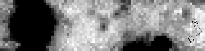
Figure 1: Average intensity image, eliminating all phase and polarization information. PSR B0656+14 is in the exact center of the image. Note the extended object which overlaps the pulsar (above the pulsar in this plot). The size of this image is 40$\times$10 arcsec (0.5 arcsec/pixel).

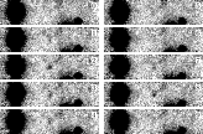
Figure 2: Phase-binned total intensity (i.e., no polarization information) images of PSR B0656+14. Each image is labeled by its phase bin index (0–9), with 0 corresponding to phase 0.0–0.1, 1 to phase 0.1–0.2, etc. PSR B0656+14 is in the exact center of each 40$\times$10 arcsec image. The intensity peaks in bins 2 and 8. The measured intensity of the bright star 14 arcsec NE of PSR B0656+14 varies by less than 0.2% over the phase bins.

The integrated image, formed by adding all of the individual images to eliminate phase and polarization information, is shown in Figure 1. The total intensity images, formed by combining sets of polarized images but retaining the 10 phase bins, are shown in Figure 2.

A 3$\times$3-pixel (1.5$\times$1.5 arcsec) aperture was used to extract the flux of PSR B0656+14 in each phase bin. While absolute photometric measurements using a small (and square) photometric aperture are difficult to calibrate, the choice of aperture does not affect the time-differential photometry, to first order. The short pulse period (0.385 s) ensures that the point spread function and image centroids are the same in all phase bins, to first order. The total intensity of a bright nearby star, measured using the same analysis routines and photometric aperture used to analyze PSR B0656+14, is measured to be constant to a signal-to-noise ratio exceeding 800. Assuming the fractional photometric errors are constant, they contribute no more than a $\sim$ 0.125% error in the PSR B0656+14 measurements. The individual polarized flux measurements from the nearby bright star are constant to a similar level ($\sim$ 0.1%). Flat-fielding and bias subtraction are performed as described in detail in Kern (2002).

3.1 Background Subtracted Pulse Profile

A nearby extended object, which is visible in Hubble Space Telescope WF/PC2 and NICMOS images of the field around PSR B0656+14 (Koptsevich et al., 2001), when observed from the ground contributes some light to the photometric aperture used for PSR B0656+14. This object is labeled o2 by Koptsevich et al. (2001). The HST WF/PC2 images were observed in the F555W filter, a similar bandpass to that of our ground-based images. We convolve the WF/PC2 images with a gaussian PSF whose FWHM equals our average ground-based seeing FWHM (1.3 arcsec). We find that in our 1.5 arcsec square photometric aperture, the extended object contributes 39% $\pm$ 7% of the pulse-averaged light in our (ground-based) photometric aperture.

We define $I_{i}$ as the background-subtracted intensity of PSR B0656+14 in phase bin $i$, which is plotted in Figure 3, normalized by the pulse-averaged flux, $\overline{I}$. The uncertainties plotted in Figure 3 are determined from the variations in the measured intensities in each phase bin, and are only 5% larger than the expected Poissonian errors due to the background flux surrounding PSR B0656+14. The phases of our observations are referenced to the peak of the radio pulse, which arrives at phase 0.0. The possible gamma-ray pulse (Ramanamurthy et al., 1996) peaks at phase 0.2. The soft X-ray pulse broadly peaks near phase 0.85, with a minimum near phase 0.3 (Marshall & Schulz, 2002).

The minimum of the normalized background-subtracted pulse profile, $I_{\rm min}/\overline{I}$, is -0.05. While a negative intensity is clearly unphysical, the measurement error in each bin ($\sigma_{I}/\overline{I}=0.24$) can account for this discrepancy. Using all of the bins in a joint probability measurement, we find a 1-$\sigma$ upper limit (two-tailed) to the true unpulsed flux to be $I_{\rm unpulsed}/\overline{I}<0.16$, accounting for both measurement error in each bin and the uncertainty in the background level. The limited temporal resolution of these measurements causes $I_{\rm unpulsed}$ to be overestimated, so this number is an upper limit.

The pulse profile we measure for PSR B0656+14 differs from that measured by Shearer et al. (1997). Due to an ephemeris folding error (A. Shearer 2002, private communication), the Shearer et al. published results must be shifted in phase so that the peak arrives at phase 0.8 (relative to the radio peak at 0.0). Shearer et al. measure a pulse with a broad single peak, similar to the soft X-ray pulse profile (Marshall & Schulz, 2002), reaching a maximum at phase 0.8, coincident with our Peak 2, but they find a minimum near phase 0.2, coincident with our Peak 1. Considering the errors in the flux levels ($\sim$ 80% of the mean flux) and the sky background level ($\sim$ 40%) published by Shearer et al., along with our errors (24% flux, 7% background), the two curves (independently normalized to the measured mean fluxes) disagree at the 97.5% (two-tailed) level. Some difference may be expected because the Shearer et al. results were obtained through a $B$ filter, while ours were obtained through a wider passband (400–600 nm). The measured disagreement could be due to the pulse morphology changing over the 5 years between the Shearer et al. observations and ours, or simply due to measurements that sample the tail of the error distribution. The level of disagreement does not warrant serious discussion of variability in the pulse morphology.

3.2 Linearly Polarized Flux

We compute the linearly polarized flux, $L_{i}$, and the polarization position angle, $\theta_{i}$, from the measured Stokes parameters $Q_{i}$ and $U_{i}$,

$$L_{i} = \sqrt{Q_{i}^{2}+U_{i}^{2}},$$ (1a)

$$\theta_{i} = \tan^{-1}(U_{i}/Q_{i})/2.$$ (1b)

Following the prescriptions in Simmons & Stewart (1985), we construct a Wardle-Kronberg (Wardle & Kronberg, 1974) estimator for $L_{i}$, which we denote $L^{\rm WK}_{i}$, to reduce bias in points with low signal-to-noise ratios. A plot of the linearly polarized flux (using the Wardle-Kronberg estimator), normalized to the pulse-averaged flux, is shown in Figure 4. In phases 0.4 – 0.7, the $L^{\rm WK}_{i}$ values differ from zero at the 2–3-$\sigma$ level.

We test the significance of the polarized flux measurements in two ways. In each test we use the simple estimator in Eqn. 1a for $L_{i}$, rather than $L^{\rm WK}_{i}$. If the uncertainties in $Q_{i}$ and $U_{i}$ are distributed as independent gaussian variables with variance $\sigma^{2}$, under the null hypothesis that there is no polarized flux, $\chi^{2}=\sum_{i=0}^{9}L_{i}^{2}/\sigma^{2}$ should be distributed as $\chi^{2}$ with 20 degrees of freedom. This first test gives $\chi^{2}=50$, which has a cumulative probability of 94.5%.

The polarized flux measurements form a time series, in which the ordering of the measurements is significant. We test the randomness of the time series (i.e., , the ordering) with the Wald-Wolfowitz test of serial correlation (Wald & Wolfowitz, 1943). The ordering of the polarization values measured violates the null hypothesis, that the numbers are randomly chosen, at the 97% level.

The combination of these two tests, which are independent of one another (the size of the measurements is independent of the ordering of the measurements), lends some credibility to the measured polarization flux values. We combine the cumulative probabilities of the two tests (94.5% and 97%) to derive a significance of 0.998 for the detection of pulsed polarized flux (a 3-$\sigma$ result).

If the position angle changes by 90° on timescales comparable to the bin width, the measured linear polarization will be reduced. Therefore, the measured linear polarization must be considered a lower limit. The best estimate is then that the flux is $\sim$ 100% polarized from phase 0.4–0.7, and (linearly) unpolarized at other phases.

4 Emission Models

There are two dominant classes of models that attempt to explain the origin of the optical emission. These two classes are the polar cap models and the outer gap models. In each of these two classes of models, the morphology and the polarization of the optical light curve are determined by the spin period, $P$, the angle between the rotation and magnetic axes, $\alpha$, and the colatitude of the observer’s line-of-sight, $\zeta$. The geometry is shown diagrammatically in Fig. 5. In addition, the polar cap model allows the height of the emission region, $h$, to vary.

The optical light curve of PSR B0656+14 is sharply double-peaked, unlike either the radio (Gould & Lyne, 1998) or the X-ray (Marshall & Schulz, 2002) light curves, which are both single-peaked. We separate the optical light curve (see Fig. 3) into 4 phase intervals. We define Peak 1 from phase 0.2–0.3, Bridge emission from phase 0.3–0.8, Peak 2 from 0.8–0.9, and Off-pulse from 0.9–1.2.

The radio pulse peaks at phase 0.0, with FWHM 0.04–0.07 at frequencies from 0.2–1.6 GHz (Gould & Lyne, 1998). The Rotating Vector Model (RVM) allows radio polarization profiles to determine the geometry of the magnetic poles relative to the rotation axis and the observer line-of-sight (LOS). In the case of PSR B0656+14, the deepest data (at 1.4 GHz) give a measurement of $\alpha=29\arcdeg\pm 23\arcdeg$, $\beta=8.9\arcdeg\pm 6.1\arcdeg$ (Everett & Weisberg, 2001), where $\beta$ is the angle of the closest approach of the observer LOS to the magnetic axis, defined by $\beta=\zeta-\alpha$. The uncertainties of these angles are highly (positively) correlated. Two earlier studies investigated PSR B0656+14, with Lyne & Manchester (1988) giving $\alpha$=8.2°, $\beta$=8.2°, and Rankin (1990) giving $\alpha$=30° (with no estimate of $\beta$.) These earlier studies do not estimate errors, as they are fits to empirical assumptions about the underlying geometry whose errors are not easily estimated.

4.1 Polar cap model

The polar cap model assumes that the optical light is emitted near the surface of the neutron star, at radii small compared to the light cylinder radius. The optical light curve and polarization information can be tested against two predictions of the polar cap model. First, the polarization position angles can be compared to the predictions of the RVM, using geometric parameters determined by radio polarization data. Second, the phase separation between the peaks in the optical light curve, combined with the geometric parameters determined by the RVM, determines an emission height for the optical peaks. If this emission height is too large to be consistent with the polar cap model, then the model fails.

The RVM is a simple model, which assumes that the polarization position angle depends only on the projection of the magnetic dipole axis on the sky. Because the position angles predicted by the RVM have no dependence on height above the neutron star surface, we can reasonably assume that the radio and optical position angles must follow the same fit, even if they are emitted in different regions. The radio polarization data of Everett & Weisberg (2001) are not calibrated with an absolute position angle, which leaves the zero-point of radio position angles as a free parameter. We take the RVM position angles predicted by the fits to the radio polarization, degrade the temporal resolution to that of the optical observations (10 resolution elements), and add a constant position angle offset to best fit the optical polarization measurements. The best-fit RVM prediction, showing both the radio and optical position angles, is shown in Figure 6. The range of $\alpha$ and $\zeta$ allowed by the radio fit does not change the predicted position angle by an amount comparable to the errors in our measurement of $\theta_{i}$, so the optical data do not reduce formal errors on $\alpha$ and $\zeta$ beyond those of the radio polarization data alone. The fit of the optical position angles to the RVM prediction is quite good, with a measured $\chi^{2}$ of 2.3 for 2 degrees of freedom (cumulative probability 0.69). The optical position angle observations greatly expand the phase coverage of the polarization data, but the size of the optical error bars and the lack of absolute calibration of the radio data angles prevent significant improvement of the RVM fit. The fact that the optical data agree well with the radio data, given that they are obtained by entirely independent techniques, does lend credibility to the RVM. The conservative conclusion drawn from the the optical polarization position angles is that they are consistent with the assumption that the optical light is emitted along dipolar field lines, without consideration of relativistic aberration, light travel time, or retarded potentials.

The polar cap model, by assuming that the light is emitted near the neutron star surface (far from the light cylinder), makes specific predictions regarding the morphology of the light curves. For the second test, the information contained in the optical pulse profile is reduced to the separation between the peaks, which are assumed to be emitted from a single height, $h_{\rm peak}$, above the neutron star surface. The last open field lines form a pseudo-cone near the surface of the star, and the optical light is assumed to be emitted along the surface of the cone (tangent to the field lines), from some height $h_{\rm peak}$ above the surface. Peaks in the optical light curve arise as the neutron star rotates and the line-of-sight intersects the cone of emission at $h_{\rm peak}$. The sharp rise of Peak 1 and sharp fall of Peak 2 match the prediction that the optical emission arises from a hollow cone (Sturner & Dermer, 1994), with the radio pulse arriving in the center of the cone, during the optical Off-pulse phase interval.

Several theoretical attempts have been made to estimate the height of the gamma-ray emission region. Recent studies have estimated that particle acceleration begins at heights 0.5–1 times the neutron star radius, $R_{\rm NS}$, above the poles (Harding & Muslimov, 1998). This particle acceleration results in radiation of curvature photons or inverse Compton scattering of thermal photons, which then produce pairs, resulting in cascades of photons and particles. The optical radiation is produced after some number of generations of this cascade. We are not aware of specific estimates of the height of the optical emission regions with respect to the primary particle acceleration regions, but it has been speculated that the gamma-ray emission regions may extend to several ($\sim$ 3–5) $R_{\rm NS}$ (Daugherty & Harding, 1996), motivated by the requirement that observed gamma-ray pulsar statistics reflect random viewing angles of pulsars. We adopt the estimate that $h_{\rm peak}\lesssim 5R_{\rm NS}$.

The opening angle of the cone defined by the last open field lines increases with increasing height, $h_{\rm peak}$, of the emission region above the neutron star surface. All else equal, larger values of $h_{\rm peak}$ result in more widely separated peaks in the optical light curve. Given values of the pulsar period, $P$, and the phase separation between the optical peaks, $\Delta\varphi_{\rm peak}$, $h_{\rm peak}$ is a function of $\alpha$ and $\zeta$. We calculate the relationship between these variables by assuming the magnetic fields are described by an inclined static dipole (defined by $\alpha$), and define the last open field lines as those which are tangent to the light cylinder (defined by $P$). We do not consider plasma loading, inertial frame dragging, or general relativistic photon propagation effects near the surface, and do not distort the field lines for any near-surface plasma effects. These additional corrections, which we neglect, can increase the opening angle of the near-surface field lines by a factor of $\sim$ 2 (Daugherty & Harding, 1996). The absence of these corrections results in conservative limits, in the sense that the corrections would allow larger values of $\alpha$ and $\zeta$ to produce the observed peak separation. For given values of $h_{\rm peak}$ and $\zeta$, we calculate the tangents to the last open field lines, and find the values of $\varphi$ for which the tangents to the last open field lines point toward the observer. Because $\alpha$ and $\zeta$ are not uniquely determined for PSR B0656+14, estimates of $h_{\rm peak}$ depend on the range of $\alpha$ and $\zeta$ allowed by the RVM. We do not use the standard small-angle approximations for the dipole field lines, but calculate the full spherical trigonometric relationships for all angles, which are valid for all values of $\alpha$ and $\zeta$.

By assuming that the optical emission forms a hollow cone (Sturner & Dermer, 1994), with the radio pulse in the center of the cone, the separation between the optical peaks becomes $\Delta\varphi_{\rm peak}=0.4$ (instead of 0.6). A plot of $h_{\rm peak}$ versus $\alpha$ and $\zeta$, showing values of $h_{\rm peak}$ comparable to several $R_{\rm NS}$, is shown in Fig. 7. It must be recognized that the uncertainties in $h_{\rm peak}$ for each $\alpha$ and $\zeta$ amount to several tens of percent, in the sense that the plot is calculated for $\Delta\varphi_{\rm peak}=0.4$, which is itself uncertain by approximately $\pm 0.1$. If $\alpha$ and $\zeta$ are less than $\sim 5^{\circ}$, $h_{\rm peak}$ is small enough to be consistent with the intial assumption of the polar cap model (that the emission region is within a few NS radii) and the constraints of the RVM.

The data contained in Fig. 7 represent only a consistency check based on the optical peak separation, from a single height above the neutron star surface. We propose an entirely empirical model to estimate the relative emissivity versus height in the polar cap model, for a range of heights. For a single representative point in Fig. 7, we calculate the emission height at all phases, defining the height as the point at which the tangent to the last open field lines points to the observer. A plot of the emission height versus $\varphi$ for $\alpha=3.5^{\circ}$, $\zeta=5^{\circ}$ is shown in Fig. 8. While this choice of $\alpha$ differs somewhat from the best-fit RVM estimate of $29\pm 23^{\circ}$ from radio data, it corresponds to $h_{\rm peak}~{}5R_{\rm NS}$, which we choose as an upper limit. For this analysis (but not in the following Outer gap model section), we make use of the lag between the radio peak and the transit of the magnetic pole, as determined from the radio polarization data in Everett & Weisberg (2001). They find that the RVM estimates a lag of $14.9\pm 0.9^{\circ}$ of the magnetic pole with respect to the radio peak, which we approximate as $\Delta\varphi$ = 0.05 (or 18^∘). We find this lag convenient, as it makes the interpretation of the pulse profile (Fig. 3) symmetric, in the sense that the first peak arrives at $\varphi\sim 0.25$ (between 0.2 and 0.3 relative to the radio peak), which is 0.2 revolutions after the magnetic pole transit, and the second peak arrives at $\varphi\sim 0.85$, which is 0.2 revolutions before the magnetic pole transit. This should not be interpreted as an independent corroboration of the estimated lag of the magnetic pole, as there is no reason to believe the profile must be symmetric, and because the effect is smaller than the optical temporal resolution.

The emissivity at different heights above the polar caps can be crudely estimated using the height profile shown in Fig. 8. We again assume light is emitted along tangents to the last open field lines. Points on the two-dimensional surface of last open field lines emit light that would be observed at different phases, $\varphi$, by observers at different colatitudes, $\zeta$. The transformation from two-dimensional area on the surface of last open field lines to solid angle ($\varphi$, $\zeta$) on the sky into which optical light is emitted defines a Jacobian, which determines the relationship between emissivity (emitted flux per unit surface area) and the flux observed in a given phase interval (recognizing that the observer defines a delta-function in $\zeta$). At lower heights, the magnetic field lines diverge more rapidly, which results in a lower observed flux for a given emissivity (i.e., , the flux is emitted into a larger solid angle). Conversely, given an observed flux, the inferred emissivity is greater at lower heights.

A plot of the estimated emissivity versus height above the neutron star surface is shown in Fig. 9, for $\alpha=3.5^{\circ}$, $\zeta=5^{\circ}$. The points at small $h$ (less than $\sim 3R_{\rm NS}$) come from the Off-pulse interval, the peaks in emissivity correspond to the optical peaks, and the largest value of $h$ corresponds to $\varphi$ = 0.5–0.6. This plot clearly shows the errors implicit in Fig. 7, based on the size of the horizontal bars (the range of heights that contribute to each phase bin). The heights and emissivities shown in Figs. 8 and 9 depend on the given geometry ($\alpha=3.5^{\circ}$, $\zeta=5^{\circ}$), but the trends in the plots remain the same for different geometries, with a rapid rise of emissivity up to $h_{\rm peak}$, declining at larger heights. It must be emphasized that this emissivity model is purely empirical, and is not based on any understanding of the underlying pair cascade physics or emission mechanisms.

4.2 Outer gap model

Outer gaps arise beyond null charge surfaces, where the Goldreich-Julian charge density vanishes (Romani & Yadigaroglu, 1995; Romani, 1996). These gaps act as accelerators, which result in cascades of high-energy particles and photons being emitted along the magnetic field lines (in the rotating frame). The gaps are “closed” some distance from the null charge surface, where the cascades supply a sufficient density of charged particles to end the acceleration. In a broad interpretation, the regions responsible for the observed optical emission are bounded by the null charge surfaces, the last open field lines, the light cylinder, and the upper edges of the gap (where the cascades close the gap). Individual models, applied to different pulsars, have assumed that high-energy emission comes from some subset of the potential emission region.

The typical assumption used to model the observed emission from an outer gap is that photons are emitted, in the rotating frame, along magnetic field lines. Calculating the resulting light curve entails applying relativistic corrections and correcting for light travel times, which means that the emission region observed at a particular phase is generally not along the line-of-sight connecting the observer to the surface of the neutron star. In addition, calculating the magnetic field line trajectories at radii comparable to the light cylinder radius requires using retarded potentials, such as those described by Deutsch (1955).

The parameters required to produce an individual light curve using an outer gap model are $P$, $\alpha$, and $\zeta$, as in the polar cap model, plus a width parameter $w$. The width parameter, $w$, identifies a set of magnetic field lines, based on the location at which they intersect the surface of the neutron star. The last open field lines are defined to lie at $w=0$, while the magnetic pole defines $w=1$ (Romani & Yadigaroglu, 1995). A given value of $w$ identifies a two-dimensional surface (a pseudo-cone), that is the collection of all magnetic field lines that strike the neutron star surface at the appropriate distance from the magnetic pole. We then assume that this surface emits optical photons tangential to the local field lines, directed inward, outward, or both, with a constant flux per unit surface area. More complex outer gap models may also include azimuthal and radial limits on the emission region inside the outer gap, or any arbitrary pattern of emission over the surfaces of constant $w$.

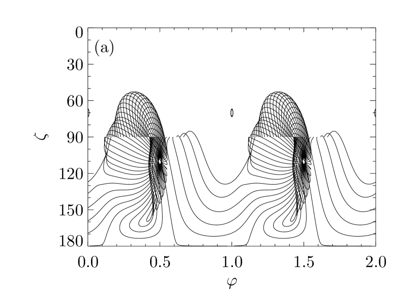
Figure 10: (a) Outward-going emission skymap for $\alpha=70^{\circ}$, $w=0.20$. Each point in the plot represents the phase, $\varphi$, at which an observer at colatitude $\zeta$ would observe an outward-going photon emitted along magnetic field lines in the $w=0.20$ surface. Only values of $\zeta<90^{\circ}$ are in the outer gap (the null-charge surface corresponds to $\zeta=90^{\circ}$), where photons are produced. The small circles at $\zeta=70^{\circ}$, $\varphi=0$, 1, and 2 represent the magnetic pole responsible for the radio emission. (b) Envelope of outer gap emission region. The lines denote the boundary between areas with observable emission and those without. These lines include virtually all peaks in the light curves. The hatched regions show the locations of the optical peaks (relative to the radio peak at $\varphi=0$). The envelope does not intersect the region $\varphi$ = 0.8–0.9 for these parameters, implying that this geometry cannot produce the observed optical peaks.

In our simplified approach, where we only determine emission peaks for a given geometry, we adopt a simple technique for identifying peaks. For a given $\alpha$ and $w$, a skymap is constructed, as described in Yadigaroglu (1997). A skymap shows the locus of points in the $\zeta$-$\varphi$ plane (where $\varphi$ is phase) which correspond to observable emission from the surface of magnetic field lines defined by $w$. The skymap corresponding to $\alpha=70^{\circ}$, $w=0.2$ is shown in Fig. 10. The transformation that maps the two-dimensional surface of magnetic field lines at constant $w$ to the two-dimensional skymap ($\zeta$ vs. $\varphi$), combined with the assumption of constant emitted flux per unit surface area, results in a map of observed flux per unit $\zeta$-$\varphi$ area. The Jacobian of this transformation is large (high flux) where $\zeta$ and $\varphi$ change little across or along magnetic field lines. This is most commonly the case at the envelope of the optical emission regions, between regions of $\zeta$ and $\varphi$ where there is observable emission and regions where there is none. We then use the location of this boundary as an estimate of the $\zeta$ and $\varphi$ at which the optical light curve peaks. One motivation for this formulation is that for a given $\zeta$, the lightcurve will be discontinuous at values of $\varphi$ which cross this boundary, as the flux is zero on one side of the boundary. While this quality does replicate part of the phenomenology associated with a peak, by only reproducing the positions of the optical peaks, we make no distinction between zero emission off-peak and bridge emission.

This simplified technique is prone to identify too many peaks. There are configurations for which the outer gap models generate broad, sinusoidal pulse profiles, whose peaks are not captured by identifying boundary crossings. In addition, there are low flux regions identified by this technique that are insignificant in the overall pulse profile. Configurations with small values of $\alpha$, or large values of $\zeta$ (near 90^∘) tend to produce more spurious peaks using this technique.

Given the large number of pulse profiles that can be constructed by varying the available parameters, we restrict the observational features we try to match. We reduce the contents of the optical light curve to the peak positions, specifically, Peak 1 occurs between phases 0.2–0.3 and Peak 2 occurs between phases 0.8–0.9. The radio pulse arrives at phase 0.0. We model the emission from three classes of outer gap models, to match the observations. Class A restricts the emission region to single values of $w$, and insists that the phases of the two optical peaks and the radio peak all match the observations. Class B allows emission from all values of $w$, and insists that the phases of the radio and optical peaks match. Class C allows emission from all values of $w$, but assumes the optical peaks have no relationship to the radio peak. For each of these classes, we determine the light curves produced by only outward-going photons, only inward-going photons, and a combination of inward- and outward-going photons. For each of the nine resulting constraints, we determine the values of $\alpha$, $\zeta$, and (for Class A) $w$ which produce the observed phases of optical peaks.

We calculate skymaps, and their corresponding envelopes, for $\alpha$ = 5^∘–85^∘ at intervals of 5^∘, and for $w$ = 0.02, 0.05, 0.10, 0.20, 0.40, and 0.80. From this grid of skymaps, we calculate peak positions for values of $\zeta$ = 1^∘–90^∘ at intervals of 1^∘. The agreement of the models with the constraints corresponding to each class, and inward- or outward-going emission, are recorded and binned into 5^∘-square bins in $\alpha$-$\zeta$ space. The results of the agreement of the models is presented in Fig. 11. We include the regions of $\alpha$ and $\zeta$ which are consistent with the RVM applied to the radio data in Fig. 11, except in Class C, which ignores the radio data.

Further work will be required to compare the observed polarization profile to those predicted by the outer gap models under different geometries, in an attempt to further constrain the outer gap models.

5 Discussion

The double-peaked nature of the optical pulse profile can be interpreted in light of both polar cap and outer gap models. In the absence of a clear gamma-ray pulse profile for PSR B0656+14, and given that the soft X-rays observed for PSR B0656+14 are commonly interpreted as thermal emission from the neutron star surface, the optical pulse profile is the only high-energy data available to test these models. The optical polarization data, while not of high signal-to-noise ratio, allow a new set of diagnostics to be applied to these tests.

Unlike the radio emission, which is probably coherent curvature radiation, the optical emission mechanism is more likely to be synchrotron radiation. This is supported in the case of PSR B0656+14 by the close match between the optical fluxes and the extrapolation of the non-thermal X-ray power law component, scaling as $\nu^{-0.45}$ (Koptsevich et al., 2001). There are two immediate implications of this inference. First, the polarization position angle differs by 90^∘ between curvature and synchrotron radiation. Curvature radiation in the normal mode is polarized parallel to the $B$ field, while the position angle of syncrotron radiation will be perpendicular to the $B$ field. We cannot test this prediction without absolutely calibrated radio position angles. Without absolutely calibrated position angles, there is no orientation against which to compare the measured optical position angles. Second, if the optical light is synchrotron with a negative power-law exponent, the $B$ field at the location of emission must be low enough that the synchrotron characteristic frequency is below the optical frequency. A critical frequency, $\nu_{\rm c}$, of $\lesssim 10^{14}$ Hz corresponds to $B\lesssim 10^{8}$ G, compared to the surface $B_{0}=5\times 10^{12}$ G. This constraint leads to a minimum height of the emission region of $\gtrsim 35R_{\rm NS}$ for the dipole field to drop to 10⁸ G.

The polar cap model can explain the morphology of the optical pulse profile, with the light arising from an emission within $\sim 5R_{\rm NS}$, for $\alpha$, $\zeta\lesssim 5^{\circ}$, as shown in Fig. 7. As is typical for polar cap models with widely separated peaks (Sturner & Dermer, 1994), the predicted values of $\alpha$ are small. What is striking is that the polarization position angles for the optical light curve agree very well with the sweep predicted by the Rotating Vector Model, applied to the radio polarizaion data of Everett & Weisberg (2001). While the agreement is quite good ($\chi^{2}$ = 2.3 for 2 degrees of freedom), it is based on only three data points, which give only two degrees of freedom because the absolute position angles of the radio data are not known. The optical position angles do support the interpretation of the radio data in Everett & Weisberg (2001), which is encouraging, as the fits to the RVM using radio data from a short phase interval give estimates with a great deal of covariance in the parameters. The simple fact that the sweep of optical position angles agrees at all with the radio position angles implies a new level of confidence that the RVM applies to PSR B0656+14, considering that the RVM gives good fits to only a small fraction of pulsars with high-quality radio polarization data. It must be recognized that the radio polarization data are obtained in only a small window of phase (see Fig. 6), while the optical position angles are taken from a wider range of phase. The optical data, when combined with the radio data, give a more complete picture than is available for nearly any other radio pulsar, except the Crab (which does not follow the RVM). While the optical data do not directly confirm the estimated lag between the radio peak and the magnetic pole transit, the agreement of the optical data with the RVM fit does bolster confidence that the RVM can be interpreted quite literally in the case of PSR B0656+14. The optical position angles do not allow us to test if the optical light is synchrotron while the radio is curvature radiation, because the radio position angles are not absolutely calibrated. Regardless of the interpretation of the optical position angles, the polar cap model can explain the general morphology of the optical light curve (peak positions relative to the radio peak, bridge emission between the peaks). However, there may be a problem with an unbroken synchrotron power-law spectrum through optical frequencies requiring a larger emission height ($\gtrsim 35R_{\rm NS}$) than is realistic under polar cap cascade scenarios ($\lesssim 5R_{\rm NS}$).

The outer gap models discussed here are somewhat restrictive, in that we do not accomodate several dimensions of flexibility available to outer gap models. We assume a constant emitted flux per unit surface area across the entire possible outer gap region. This assumption ignores, for example, the flexibility allowed by instituting azimuthal or radial limits to the optical emission region, which could shift the location of the peaks in the optical light curve. We also reduce the optical light curve to its simplest observable parameter, the location of the optical peaks. We find that with these restrictions, we are able to find agreement between the data and the outer gap models, as summarized in Fig. 11. However, in examining only the presence of peaks at the observed phases, we ignore the fact that most of these models produce too many peaks. For instance, the inclusion of both outward- and inward-going emission produces four peaks for most geometries. In addition, including many values of $w$ in the calculations (which results in many geometries compatible with the observations) would diffuse the peaks, without fine-tuning the models by restricting the emission region in azimuth or radius. The overly liberal approach we take in our modeling, which produces as many peaks as possible, is intended only to determine the ability to construct a model which produces peaks at the right positions, with the assumption that the remaining degrees of freedom could be used to fine-tune the model to better fit the entire light curve observed.

One conclusion that is not well represented in Fig. 11 is that values of $w>0.40$ do not contribute significantly to the observed optical peaks. Zhang & Cheng (1997) predict that because PSR B0656+14 rotates slowly, 70% of the volume of the outer magnetosphere should be filled by the outer gap. While this fractional volume is not directly comparable to $w$, taken simplistically, it seems to imply that the optical emission is being emitted well inside (i.e., not filling) the boundaries of the outer gap.

The Crab Pulsar is the only other pulsar for which optical polarization measurements are available. The polarization pulse profile measured in PSR B0656+14 is different in character than that measured in the Crab. The Crab’s linearly polarized flux is maximized at the peaks and minimized in the bridge, while the polarized fraction is maximized in the bridge and minimized at the peaks (Smith et al., 1988). In PSR B0656+14, the linearly polarized flux and polarized fraction are both maximized in the bridge and both minimized at the peaks. The low temporal resolution of our optical measurements will lead to a decrease in the measured linearly polarized flux, but our observations of the Crab at the same temporal resolution show a much greater polarized flux at the peaks (where the position angle swings rapidly) than in the bridge. Under the RVM, this decrease in measured linearly polarized flux would be small, as can be seen by noting that the position angle sweep is not rapid at phases 0.2 and 0.8 in Fig. 6. However, the RVM does not apply to the position angles measured in the Crab (as the position angles execute a “double sweep”), so without a more detailed polarization model for PSR B0656+14, we cannot rule out the chance that rapid swings have degraded our measured polarized flux.

The 1-$\sigma$ upper limit on the unpulsed flux is 16%, limiting the contribution of thermal radiation to the observed flux. As we are presenting only differential photometry in these observations, we must rely on absolute photometry presented by other authors, which almost certainly have different methods of background subtraction (and treatment of the nearby extended object). As such, we note only that this limit on the thermal radiation from PSR B0656+14 is not surprising, given realistic extrapolations of the Rayleight-Jeans emission (Koptsevich et al., 2001). The high pulsed fraction does, however, rule out models in which the optical emission is due to a fallback disk (Perna, Hernquist, & Narayan 2000). A comparable pulsed / unpulsed measurement in the UV would provide a much better constraint on the Rayleigh-Jeans tail of the thermal emission from the surface of PSR B0656+14.

Figure 3: Total-intensity pulse profile of PSR B0656+14. The intensity scale is normalized to the pulse-averaged intensity. Error bars are 1-$\sigma$ errors. Pulse is plotted twice for clarity. All intensities have been background-subtracted as described in Section 3.1. The radio pulse peaks at phase 0.0, and the possible gamma-ray peak (Ramanamurthy et al., 1996) is at phase 0.2.

Figure 4: Linearly polarized flux. The filled circles are the Wardle-Kronberg estimates of the linearly polarized flux, $L^{\rm WK}_{i}$, with 1-$\sigma$ error bars, normalized to the pulse-averaged total intensity. The dotted line is the total-intensity pulse profile, on the same flux scale, duplicated from Fig. 3.

Figure 5: Rotation geometry. $\Omega$ is the rotation axis, $\mu$ is the magnetic axis, $\alpha$ is the angle between $\Omega$ and $\mu$, and $\zeta$ is the angle between $\Omega$ and the observer’s line-of-sight.

Figure 6: Linear polarization position angles, $\theta$. Diamonds are the optical position angles with 1-$\sigma$ error bars, dots are the radio polarization position angles from Everett & Weisberg (2001). The radio position angles are not absolutely calibrated, and are shown with the best-fit zero-point offset. The radio position angles do not have error bars plotted. The radio position angle measurements made where the radio flux is low ($|\varphi|>0.05$) have large uncertainties. The dotted line is the prediction from the Rotating Vector Model, using the radio data. The solid line is the same prediction, with temporal resolution reduced to equal that of the optical measurements.

Figure 7: Height at which optical peaks are emitted. Contours represent heights of the optical emission region, above the surface of the neutron star, that give the observed phase separation between peaks of 0.4. The heights are stated in multiples of $R_{\rm NS}=10$ km. The hatched region is the 3-$\sigma$ confidence region for $\alpha$ and $\zeta$ (no dependence on $h_{\rm peak}$), applying the Rotating Vector Model to the radio data of Everett & Weisberg (2001). The cross-hatched region denotes $h_{\rm peak}<0$, for which there is no geometry giving the observed peak separation. This plot shows only values of $\alpha$ and $\zeta$ corresponding to a range of $h_{\rm peak}$ comparable to the theoretically expected heights.

Figure 8: Sample optical emission height profile in polar cap model. This plot is calculated for $\alpha=3.5^{\circ}$, $\zeta=5^{\circ}$ (see Fig. 7), assuming the magnetic pole transit lags the radio peak by 0.05 in phase. The height, $h$, at which the tangent to the last open field lines point to the observer, is plotted versus phase, $\varphi$, normalized to the neutron star radius, $R_{\rm NS}$ = 10 km. The vertical dotted lines correspond to the nominal locations of the optical peaks (during the phase intervals 0.2–0.3, and 0.8–0.9), and the hatched regions approximately mark the Off-pulse interval.

Figure 9: Sample areal emissivity versus height in polar cap model. The emissivity is calculated from the observed pulse profile (Fig. 3) and the Jacobian of the transformation from area on the last closed field lines (at the emission location as defined in Fig. 8) to solid angle on the sky. The geometric assumptions are as in Fig. 8, and the plotted values vary as $\alpha$ and $\zeta$ vary. Ten points are plotted, corresponding to the ten measured points in the pulse profile. The vertical error bars are the 1-$\sigma$ errors from Fig. 3, the horizontal bars denote the range of heights associated with the phase interval in each phase bin.

Figure 11: Outer gap parameters which match observed optical properties. Each panel is marked at values of $\alpha$ and $\zeta$ for which the outer gap models can produce a light curve with peaks at the observed phases. The (a) panels produce peaks at phases 0.2 and 0.8 relative to the radio peak at phase 0.0, from field lines at a single value of $w$. The (b) panels produce peaks at phases 0.2 and 0.8 relative to the radio peak at 0.0, from field lines at all values of $w$. The (c) panels produce peaks separated by 0.4 (or, equivaliently, 0.6) in phase, with no specified relationship to the radio peak, and from all $w$. The (1) panels show only outward-going emission, the (2) panels only inward-going emission, and the (3) panels both inward- and outward-going emission. In the (a) panels, the symbols represent the value of $w$ satisfying the observations, with a diamond for 0.02, plus for 0.05, square for 0.10, cross for 0.20, and a circle for 0.40. No models with $w=0.80$ fall on this plot. The sole data point in panel (a1) is likely to be spurious. The region in the (a) and (b) panels marked by the dotted lines is the 3-$\sigma$ confidence interval determined from the RVM fits to radio data.

References

- Becker & Trümper (1997) Becker, W. & Trümper, J. 1997, A&A, 326, 682
- Cocke et al. (1969) Cocke, W., Disney, M., & Taylor, D. 1969, Nature, 221, 525
- Daugherty & Harding (1994) Daugherty, J. K. & Harding, A. K. 1994, ApJ, 429, 325
- Daugherty & Harding (1996) Daugherty, J. K. & Harding, A. K. 1996, ApJ, 458, 278
- Deutsch (1955) Deutsch, A. J. 1955, Annales d’Astrophysique, 18, 1
- Everett & Weisberg (2001) Everett, J. E. & Weisberg, J. M. 2001, ApJ, 553, 341
- Gould & Lyne (1998) Gould, D. M. & Lyne, A. G. 1998, MNRAS, 301, 235
- Harding & Muslimov (1998) Harding, A. K. & Muslimov, A. G. 1998, ApJ, 508, 328
- Kern (2002) Kern, B. 2002, Ph.D. thesis, California Institute of Technology
- Kijak & Gil (1997) Kijak, J. & Gil, J. 1997, MNRAS, 288, 631
- Koptsevich et al. (2001) Koptsevich, A. B., Pavlov, G. G., Zharikov, S. V., Sokolov, V. V., Shibanov, Y. A., & Kurt, V. G. 2001, A&A, 370, 1004
- Lyne & Manchester (1988) Lyne, A. G. & Manchester, R. N. 1988, MNRAS, 234, 477
- Marshall & Schulz (2002) Marshall, H. L. & Schulz, N. S. 2002, ApJ, 574, 377
- Middleditch & Pennypacker (1985) Middleditch, J. & Pennypacker, C. 1985, Nature, 313, 659
- Perna et al. (2000) Perna, R., Hernquist, L., & Narayan, R. 2000, ApJ, 541, 344
- Radhakrishnan & Cooke (1969) Radhakrishnan, V. & Cooke, D. J. 1969, Astrophys. Lett., 3, 225
- Ramanamurthy et al. (1996) Ramanamurthy, P. V., Fichtel, C. E., Kniffen, D. A., Sreekumar, P., & Thompson, D. J. 1996, ApJ, 458, 755
- Rankin (1990) Rankin, J. M. 1990, ApJ, 352, 247
- Romani (1996) Romani, R. W. 1996, ApJ, 470, 469
- Romani & Yadigaroglu (1995) Romani, R. W. & Yadigaroglu, I.-A. 1995, ApJ, 438, 314
- Shearer et al. (1997) Shearer, A. et al. 1997, ApJ, 487, L181
- Shearer et al. (1998) Shearer, A., Golden, A., Harfst, S., Butler, R., Redfern, R. M., O’Sullivan, C. M. M., Beskin, G. M., Neizvestny, S. I., Neustroev, V. V., Plokhotnichenko, V. L., Cullum, M., & Danks, A. 1998, A&A, 335, L21
- Simmons & Stewart (1985) Simmons, J. F. L. & Stewart, B. G. 1985, A&A, 142, 100
- Smith et al. (1988) Smith, F. G., Jones, D. H. P., Dick, J. S. B., & Pike, C. D. 1988, MNRAS, 233, 305
- Sturner & Dermer (1994) Sturner, S. J. & Dermer, C. D. 1994, ApJ, 420, L79
- Thompson (2001) Thompson, D. J. 2001, in AIP Conf. Proc. 558, High Energy Gamma-Ray Astronomy, ed. F. A. Aharonian & H. J. Völk (Melville:AIP), 103
- Wald & Wolfowitz (1943) Wald, A. & Wolfowitz, J. 1943, Annals of Mathematical Statistics, 14, 378
- Wallace et al. (1977) Wallace, P. T., Peterson, B. A., Murdin, P. G., Danziger, I. J., Manchester, R. N., Lyne, A. G., Goss, W. M., Smith, F. G., Disney, M. J., Hartley, K. F., Jones, D. H. P., & Wellgate, G. W. 1977, Nature, 266, 692
- Wang et al. (1998) Wang, F. Y.-H., Ruderman, M., Halpern, J. P., & Zhu, T. 1998, ApJ, 498, 373
- Wardle & Kronberg (1974) Wardle, J. F. C. & Kronberg, P. P. 1974, ApJ, 194, 249
- Yadigaroglu (1997) Yadigaroglu, I.-A. 1997, Ph.D. thesis, Stanford Univ.
- Zhang & Cheng (1997) Zhang, L. & Cheng, K. S. 1997, ApJ, 487, 370