The $K$–selected Butcher-Oemler Effect

Abstract

We investigate the Butcher-Oemler effect using samples of galaxies brighter than observed frame $K^{*}+1.5$ in 33 clusters at $0.1\lesssim z\lesssim 0.9$. We attempt to duplicate as closely as possible the methodology of Butcher & Oemler. Apart from selecting in the $K$-band, the most important difference is that we use a brightness limit fixed at 1.5 magnitudes below an observed frame $K^{\ast}$ rather than the nominal limit of rest frame $M(V)=-20$ used by Butcher & Oemler. For an early type galaxy at $z=0.1$ our sample cutoff is 0.2 magnitudes brighter than rest frame $M(V)=-20$, while at $z=0.9$ our cutoff is 0.9 magnitudes brighter. If the blue galaxies tend to be faint, then the difference in magnitude limits should result in our measuring lower blue fractions. A more minor difference from the Butcher & Oemler methodology is that the area covered by our galaxy samples has a radius of 0.5 or 0.7 Mpc at all redshifts rather than $R_{30}$, the radius containing 30% of the cluster population. In practice our field sizes are generally similar to those used by Butcher & Oemler.

We find the fraction of blue galaxies in our $K$-selected samples to be lower on average than that derived from several optically selected samples, and that it shows little trend with redshift. However, at the redshifts $z<0.6$ where our sample overlaps with that of Butcher & Oemler, the difference in $f_{B}$ as determined from our $K$-selected samples and those of Butcher & Oemler is much reduced. The large scatter in the measured $f_{B}$, even in small redshift ranges, in our study indicates that determining the $f_{B}$ for a much larger sample of clusters from $K$-selected galaxy samples is important.

As a test of our methods, our data allow us to construct optically-selected samples down to rest frame $M(V)=-20$, as used by Butcher & Oemler, for four clusters that are common between our sample and that of Butcher & Oemler. For these rest $V$ selected samples, we find similar fractions of blue galaxies to Butcher & Oemler, while the $K$ selected samples for the same 4 clusters yield blue fractions which are typically half as large. This comparison indicates that selecting in the $K$-band is the primary difference between our study and previous optically-based studies of the Butcher & Oemler effect.

Selecting in the observed $K$-band is more nearly a process of selecting galaxies by their mass than is the case for optically-selected samples. Our results suggest that the Butcher-Oemler effect is at least partly due to low mass galaxies whose optical luminosities are boosted. These lower mass galaxies could evolve into the rich dwarf population observed in nearby clusters.

1 Introduction

In the late 1970’s a variety of new imaging technologies were being tried out, with an order of magnitude or more better sensitivity than photographic plates. Butcher & Oemler’s (1978) observations of two galaxy clusters at $z\sim 0.4$ using the ISIT Vidicon on the KPNO 2.1 m altered the landscape for studies of distant galaxies, providing the first clear indication of dramatic changes in galaxy properties, and in the unexpectedly recent past. Butcher & Oemler (1984; hereafter BO84) confirmed the reality of the effect by addressing a number of concerns about systematic effects in the analysis procedure, and by broadening the sample both in number and redshift. The Butcher-Oemler (BO) effect—the discovery that galaxy clusters at $z>0.2$ contain a higher fraction of blue galaxies ($f_{B}$) than do nearby galaxy clusters—inspired an empirical approach to galaxy evolution which continues to the present day.

The origin of the BO effect is important to discern. Larson, Tinsley, & Caldwell (1980) suggested that S0s could be later type disks transformed by the cluster environment into earlier types. The fraction of blue galaxies in $z\sim 0.4$ clusters is qualitatively similar to the excess of lenticulars (S0) in nearby clusters relative to those at $z\sim 0.5$ (Dressler et al., 1997), supporting the idea that infalling field spirals are transformed into S0s. Morphological transformation from spiral to S0 may be induced by starbursts occurring upon cluster infall and leading to the rapid exhaustion of gas reservoirs (Dressler & Gunn, 1983; Barger et al., 1996; Poggianti et al., 1999), by truncation of normal star formation after infall (Abraham et al., 1996; Morris et al, 1998), or by a gradual decline in star formation as the dark haloes surrounding spirals are removed and gas supplies can no longer be replenished by cooling and infall (Larson et al., 1980; Balogh et al., 2000). These mechanisms also provide natural explanations for the origin of the morphology-density relation (Dressler, 1980) and agree with the apparent preference of the blue galaxies for the outskirts of clusters (BO84). The starburst explanation is supported by spectroscopy of the blue galaxies indicating that they are seen during or shortly after an episode of star formation (Couch & Sharples, 1987; Couch et al., 1994, 1998) (hereinafter CS87, C94, and C98 respectively). Finally, $HST$ images indicate that the blue galaxies are predominantly normal late-type disks, with some tendency to be involved in interactions (Lavery & Henry 1988, Oemler et al. 1997, C94, C98).

On the other hand, Rakos et al. (1997) and C98 conclude that many of the most actively star forming blue galaxies are actually low luminosity systems, temporarily brightened by starbursts, which will fade from view and evolve not into S0s but into dwarf galaxies. In this bursting dwarf scenario the optical luminosities of such galaxies are boosted to enter the luminosity cut defined by BO84. This raises the possibility that at least part of the BO effect is a result of photometric selection. In BO84 selection is carried out in optical passbands, which could magnify the effect of even minor starbursts (even though the BO84 passbands correspond approximately to the rest-frame $V$ band).

Our understanding of the physical mechanisms responsible for the BO effect remains contentious. Part of the problem is simply that there is a wide range in measured blue fractions at a given redshift. This could be explained by the larger problem that the cluster samples usually used in studies of the BO effect do not consist of the same kind of clusters over the redshift range of interest. Andreon & Ettori’s (1999) analysis of the clusters in BO84 using X-ray data indicate that the latter’s results are biased. They found that the $L_{x}$ of the BO84 sample increases with redshift, whereas there is no evidence for evolution in the X-ray luminosity function up to $z\sim 0.8$. When Andreon & Ettori (1999) add X-ray selected clusters to the BO84 sample, the trend of the blue fraction with redshift is much reduced. Margoniner & de Carvalho (2000) found similar results, underscoring the need for a study of the BO effect using a well-defined sample of clusters, over a large redshift range. Further illustrating the importance of sample selection, Margoniner et al. (2001) found a strong correlation between cluster richness and the blue fraction, in the sense that $f_{B}$ is higher for poorer clusters, using a large sample of 295 Abell clusters.

Selection of galaxy samples in the near-infrared as opposed to the optical should result in samples more representative by stellar mass (Aragon-Salamanca et al., 1991; Gavazzi et al., 1996; Stanford et al., 1998). Stanford et al. (1998) and De Propris et al. (1999) have shown that the luminosities and colors of galaxies selected in the $K$ band are not strongly dependent on their environment. Therefore $K$-selected samples can be used to constrain the masses of the blue galaxies causing the BO effect and investigate if these objects evolve into S0’s or dwarfs.

We present here a study of the BO effect in distant clusters using galaxies selected in the $K$ band. Our sample, observations and data reduction are described in the next section. The analysis and the main results are presented in Section 3. We discuss our findings in Section 4. For consistency with BO84, we adopt a cosmology with $H_{0}=50$ km s^-1 Mpc^-1 and $q_{0}=0.1$.

2 Data

Our sample is the heterogeneous set of clusters which were studied for luminosity function evolution by De Propris et al. (1999). For this sample, we have $JK$ and two optical bands of imaging which reach at least to 1.5 magnitudes below an evolving $K^{\ast}$ at the 5$\sigma$ level. The optical bands change with redshift, bracketing the 4000 ${\rm\AA}$ break as closely as possible. Catalogs for these clusters were generated from the $K$-band images. The observations, data reduction, and photometry for this sample are presented in Stanford et al. (2002).

3 Analysis

In our analysis we are attempting to duplicate the methodology of BO84 as closely as possible. To that end, we begin with a summary of the cluster sample and procedures used by BO84. Their sample consisted of 33 clusters spanning the range $0.003\ {\rm(Virgo)}<z<0.54$ drawn mostly from the Abell catalog. The data used by BO84 came from three main sources. Except for CL0016+16 (photographic plates were obtained by Koo 1981), the most distant clusters were observed with the ISIT Vidicon camera on the Kitt Peak 2.1 m telescope in the $V$ and $R$ bands covering areas of $\sim$6.2 arcmin² down to a limit of $R\sim 22.0$. The photometry for their intermediate redshift clusters was obtained using $J$ and $F$ plates on the 4 m telescopes at KPNO and CTIO and covered areas of 55 arcmin² down to a red magnitude of 22. The photometry for the low redshift clusters was obtained from $J$ and $F$ plates done at the Palomar 1.2 m Schmidt and covered areas of radius 1.5 Mpc.

BO84 defined ‘blue’ galaxies as (i) objects lying within a radius containing 30% of the cluster population (R₃₀); (ii) brighter than a no-evolution $M_{V}=-20$; and (iii) bluer by 0.2 magnitudes in rest frame $B-V$ than the red sequence defined by the cluster E/S0 galaxies. BO84 derived the slope and intercept of the color-magnitude relation from their data or from the unevolved slope of the relation in nearby clusters (Sandage & Visvanathan, 1978) and calculated their $B-V$ color offset using spectral energy distributions from Coleman et al. (1980) and assuming no evolution.

Because of the smaller size of infrared detectors, we are generally unable to cover enough field to trace the surface density distribution of galaxies and derive $R_{30}$ directly from our data. Therefore we adopt circular apertures of radius 0.5 and 0.7 Mpc centered on the brightest cluster galaxy. The $R_{30}$ listed in Table 1 of BO84 are between $\sim$1 and $\sim$5 arcmin with an average of 2.2 arcmin for the clusters at $z>0.2$ (see our Table 2 for the $R_{30}$ of the comparison clusters). A radius $=0.7$ Mpc is very similar to this average $R_{30}$ in the redshift range where our sample overlaps with that of BO84.

As for the magnitude limit for our samples, first we need to convert from the optical band used in BO84 to the $K$-band we are using for galaxy selection. We calculate that $M_{V}=-20$ corresponds to $M_{K}=-23.05$ for early-type galaxies in the present epoch, based on data from the $UBVRIzJHK$ survey of the Coma cluster by Eisenhardt et al. (2003). Our data on the distant clusters do not reach $M_{K}=-23.05$ in all cases. We choose to use a magnitude cut at $K^{*}+1.5$, where $K^{*}$ has been determined from our data on each cluster (De Propris et al., 1999). Table 1 gives these $K^{\ast}$, along with both the limiting $K$ actually used with our data in calculating blue fractions, the observed frame $K$ magnitude that is equivalent to the nominal $M(V)=-20.0$ for an elliptical galaxy assuming pure $k-$correction (using the models of Poggianti 1997) of the observed colors of Coma early-types, and the observed frame $K$ equivalent to the actual limits in $M(V)$ used by BO84 (see Table 2). For $0.1<z<0.3$ our limiting magnitudes are somewhat brighter than those used in BO84, a point we will return to later. While different from the fixed absolute magnitude cut used by BO84, our variable magnitude limit accounts for the passive evolution seen in cluster galaxies (e.g., Stanford et al. 1998). The single absolute magnitude limit used by BO84 translates into a cut relative to $M^{\ast}$ that changes with redshift, thus possibly including variable proportions of giant and dwarf galaxies into their samples, whereas our magnitude limit is more likely to sample similar populations at all redshifts.

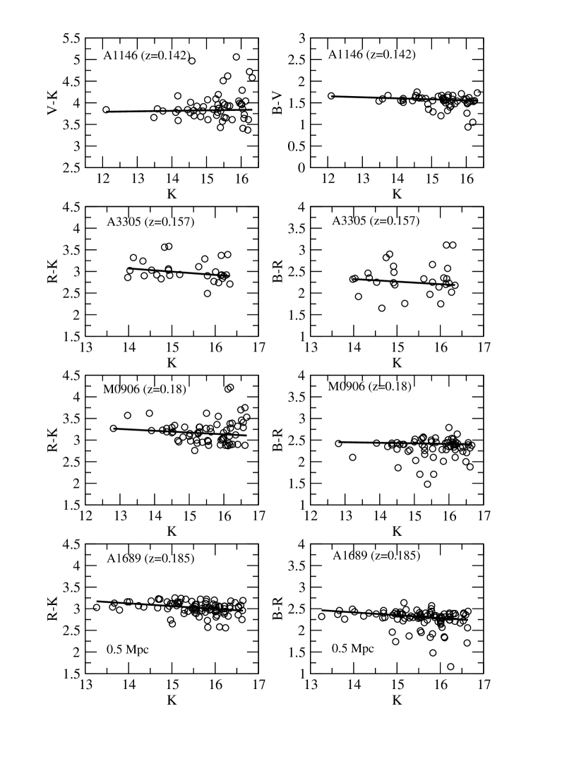
Figure 1: Color–magnitude diagrams, with best fits to the color-magnitude relation shown by the solid line, in optical-$K$ vs. $K$ and in an optical color ($B-R$, $g-$, $V-I$ or $R-I$) straddling the 4000 Å break vs. $K$ for all sample clusters. The data are for the 0.7 Mpc regions described in the text (unless otherwise specified) and to the magnitude limit referred to in Table 1.

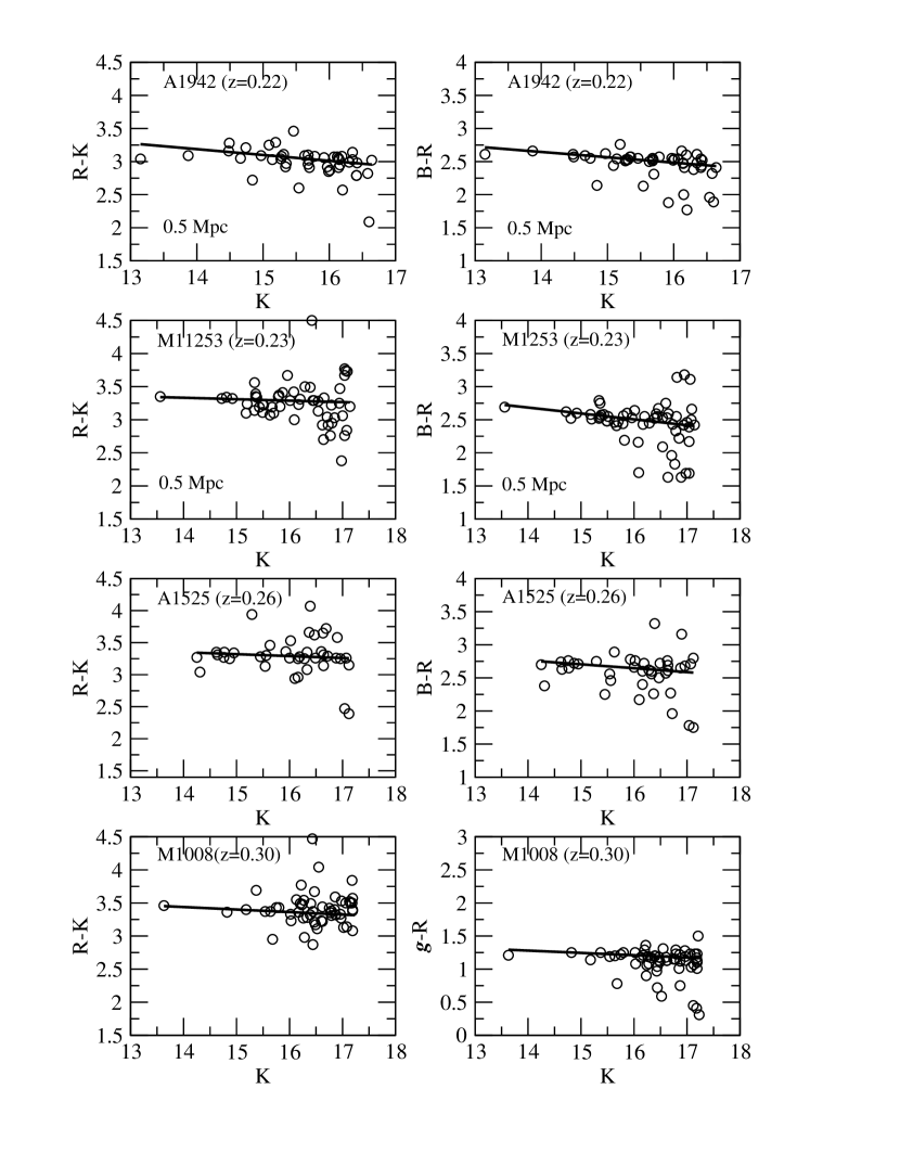
Figure 1: continued

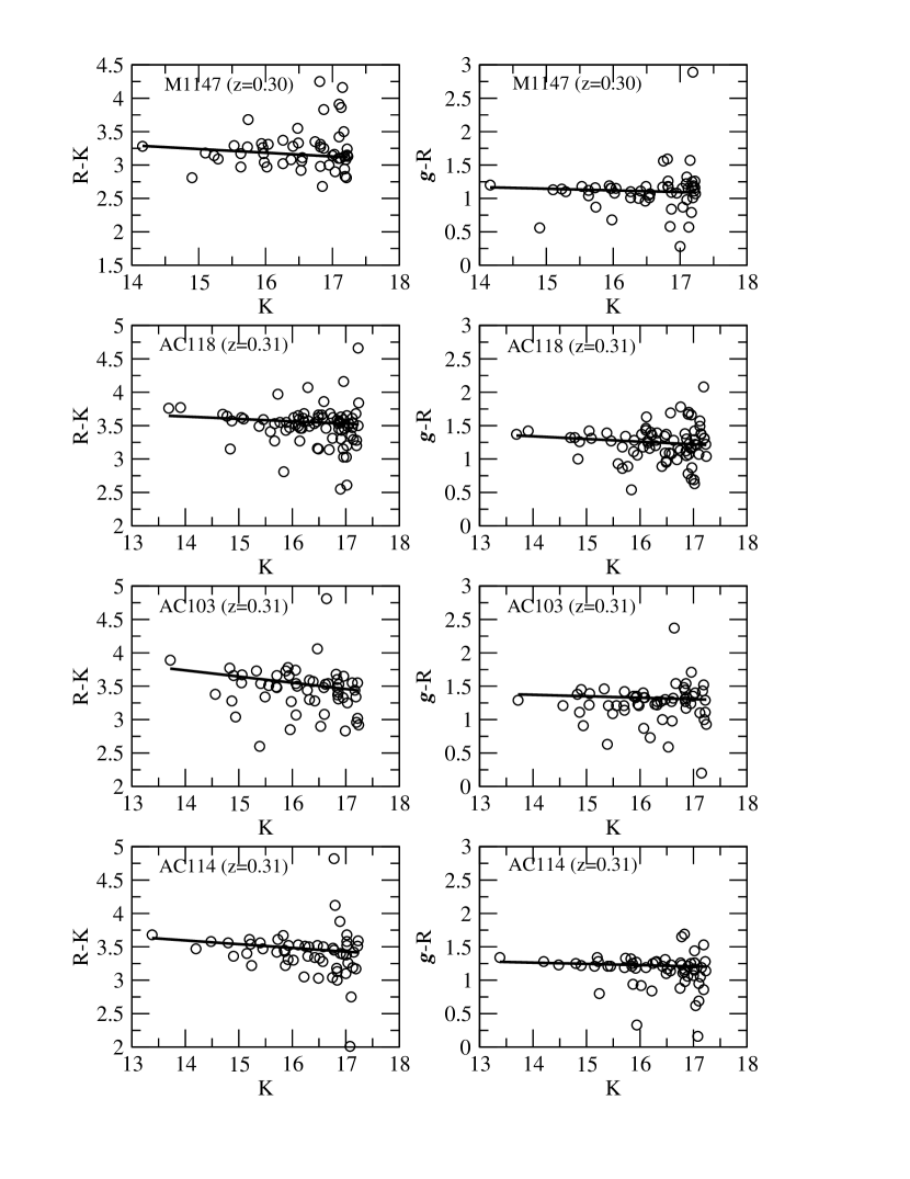
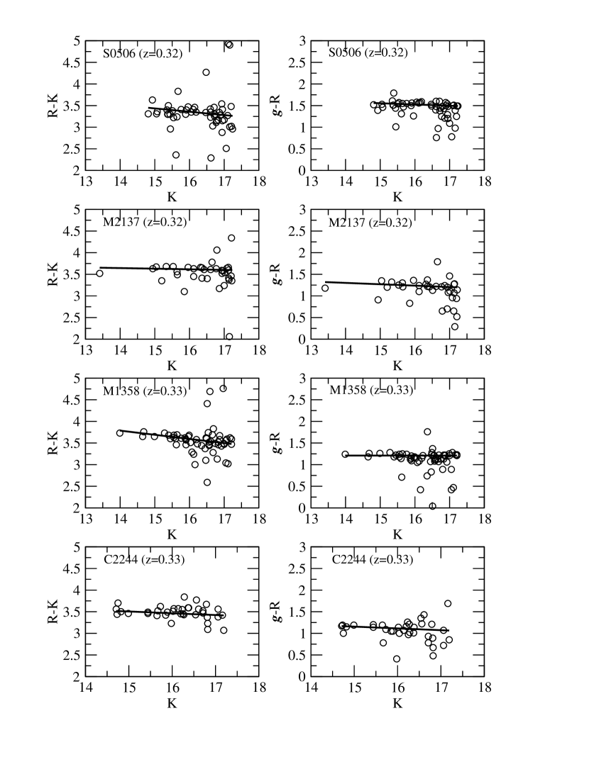
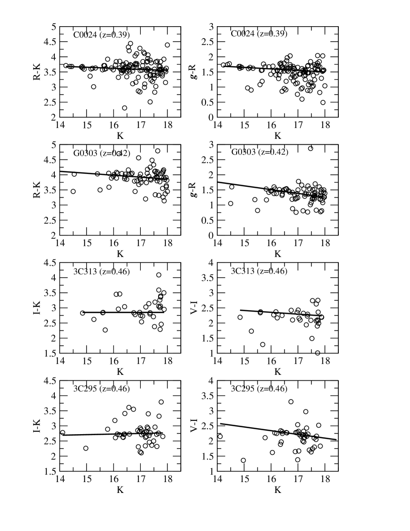
Figure 1: continued

Figure 1: continued

Figure 1: continued

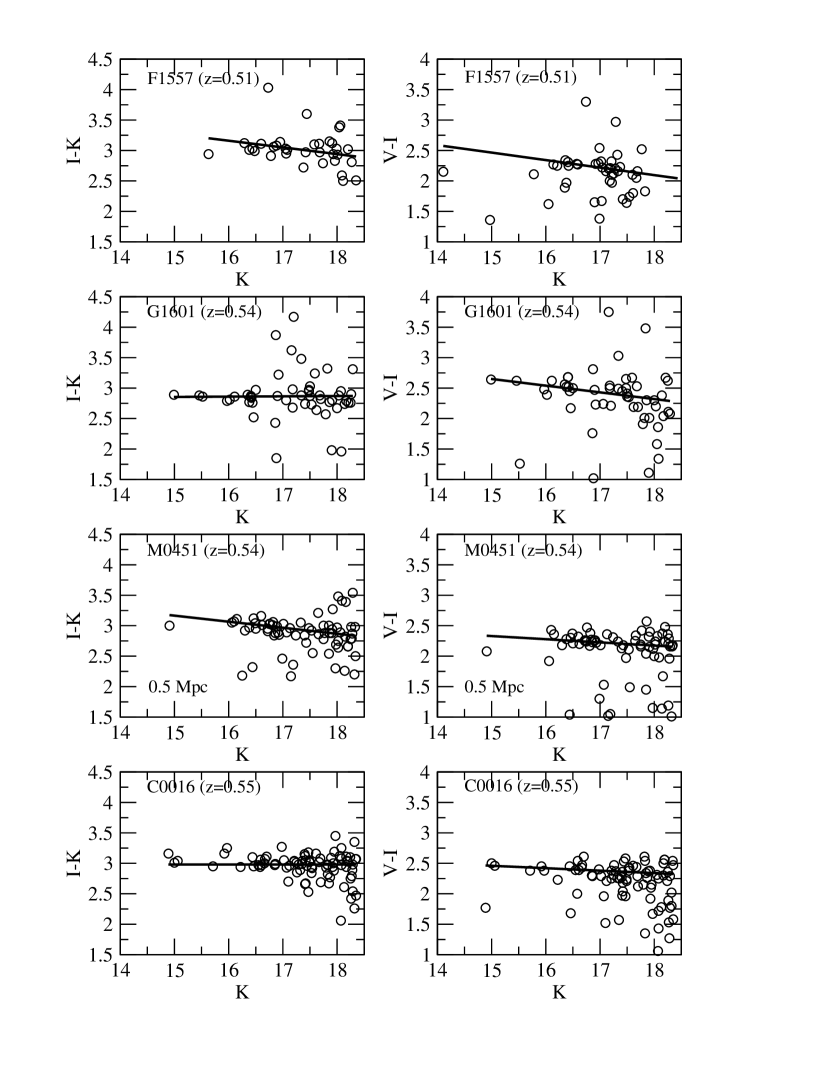
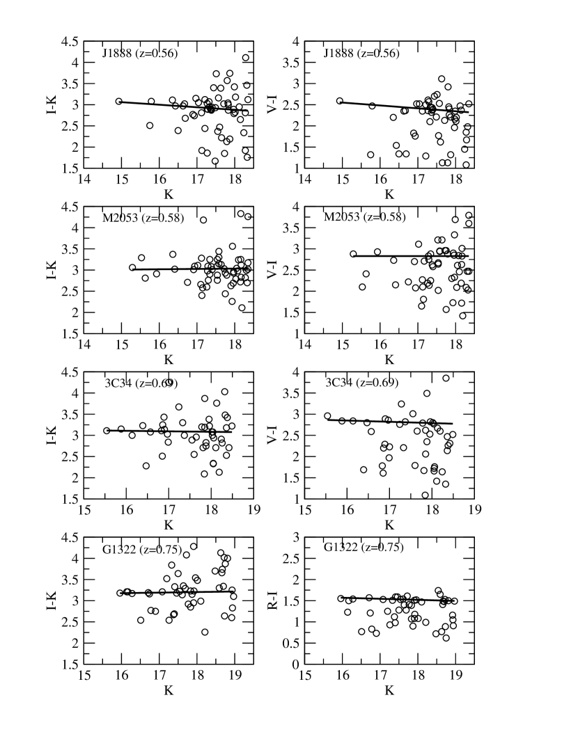
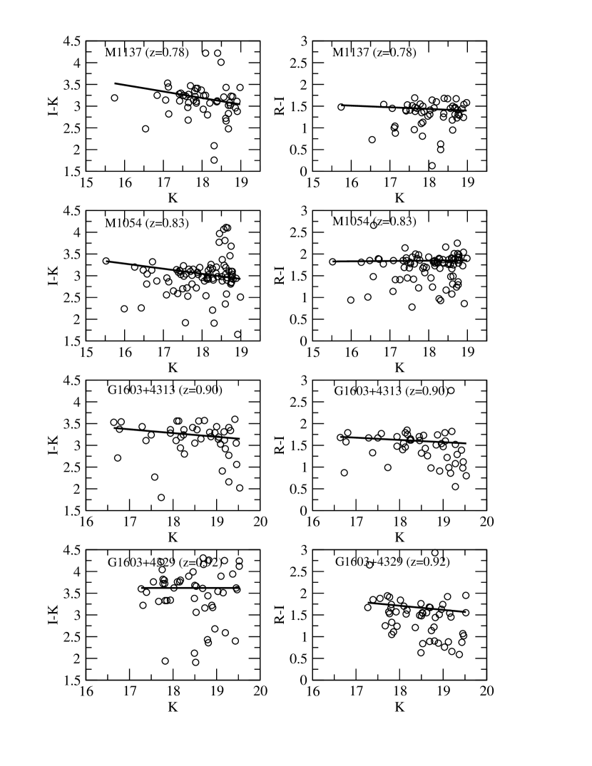
Figure 1: continued

To determine which galaxies in our samples defined by the magnitude and area limits described above are blue we follow the methodology of BO84. First we correct the galaxy colors for the color-magnitude correlation of E/S0 galaxies by fitting the optical and optical-IR colors with a robust linear least squares routine with brightest cluster galaxies excluded from the fits. This algorithm minimizes least absolute deviation (rather than its square) with iterative rejection (Applied Statistics algorithm # 132) and therefore reduces the influence of outliers. We carry out this fit within the 0.5 Mpc region to maximize the strength of the cluster red sequence. We inspect the fit by eye and, occasionally, intervene manually to produce a more acceptable relation (i.e. one where the mode of the marginalized color distribution is as close as possible to 0). The fit should be done only to the early-type galaxies but we do not have morphological information on all the clusters in our sample. The color-magnitude diagrams and the best fits are shown in Figure 1 for both the optical-IR and the pure optical colors.

In order to set a color boundary that defines the blue galaxies for our chosen passbands, we need to transform the rest frame $(B-V)=0.2$ offset into a difference in the observed colors ($B-R$, $g-R$, $V-I$, $R-I$, $R-K$ and $I-K$ as described below) at the redshift of each cluster. We follow the procedure outlined by BO84 and Smail et al. (1998) and use E, Sa and Sc spectral energy distributions from Poggianti (1997). We find that a mixture of 55% Sa and 45% Sc yields a spectrum with a color difference $\Delta(B-V)=0.2$ from an E model. We use this mixed spectrum to calculate the corresponding $\Delta\ (color)$ (for our observed colors) at $z=0$. We then use the $k-$ corrections given in Poggianti (1997) (for no-evolution models) to calculate a color difference as a function of redshift (i.e., we compute the no-evolution colors for the E model and for the Sa+Sc mixture). For example, the difference corresponding to an offset of $(B-V)=0.2$ in the observed $V-I$ at $z=0$ is 0.21 mag. For a solar metallicity elliptical in e.g. GHO1601+4253 the $k-$correction in $V$ is 1.77 mag and 0.41 in $I$ (Poggianti 1997); for the composite Sa+Sc spectrum the $k-$correction is 1.24 in $V$ and 0.21 in $I$. Therefore the $k-$corrected difference corresponding to $(B-V)=0.2$ is 0.54 magnitudes in $V-I$ at $z=0.54$.

We remove contamination from field galaxies by using the SPICES survey (Stern et al., 2002; Eisenhardt et al., 2003). SPICES is an imaging survey of four fields (Cetus, Lynx, Pisces, and SA57) in $BRIzJK$. Objects in these fields were selected in the $K$ band down to $K=20.0$, where the completeness level is $80$%. These objects were photometered in the same manner as was done for the clusters in our sample (Stanford et al., 2002). Before being used for background correction, color distributions for the field galaxy samples are corrected for the color-magnitude relations derived for each cluster. We have no $g$ or $V$ data in the SPICES field survey and so need to interpolate magnitudes for those bands for the clusters which have $g$ or $V$ data. As part of the analysis of SPICES data, photometric redshifts have been determined by A. Connolly using the methods of Connolly & Szalay (1999) and Csabai et al. (2000). This process yields spectral types as well photometric redshifts. Using these spectral types and the Coleman et al. (1980) spectral energy distributions, we may calculate colors in any band for the objects in the SPICES catalogs. As a test of this procedure, we show a comparison of interpolated and measured colors in Figure 2. The average of the differences amounts to only a few hundredths of a magnitude with an rms varying from 0.15 to 0.3 mags (as shown in the figure). This indicates that the interpolated $g$ and $V$ band colors of the field galaxies in the SPICES sample are reasonably accurate. The above rms values are typically 2–3 times smaller than the actual offsets in the observed colors that are used in determining which are the blue galaxies when calculating Butcher-Oemler fractions.

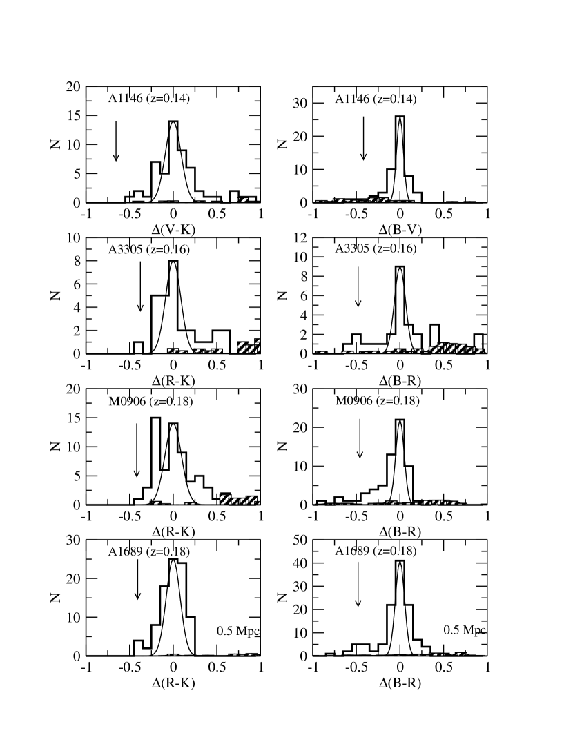
Figure 3: Marginal color distributions in optical-$K$ and an optical color straddling the 4000 Å  break for galaxies in the cluster fields (open histogram) and in the background fields (hatched histogram). We have removed the color–magnitude relations from both the cluster and field datasets and normalized field counts to the areas covered. Here we show the distributions for the 0.7 Mpc areas we use in our analysis (except for a few clusters where our data cover only 0.5 Mpc; these are identified in the figure). The arrow indicates the $k$-corrected color for galaxies to be considered ‘blue’ as per the definition of BO84 (see text for details). A Gaussian is shown centered at 0 in the marginal color with a width specified by the expected scatter in the observed colors due only to measurement uncertainties.

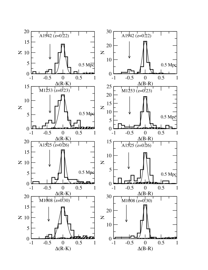
Figure 3: continued

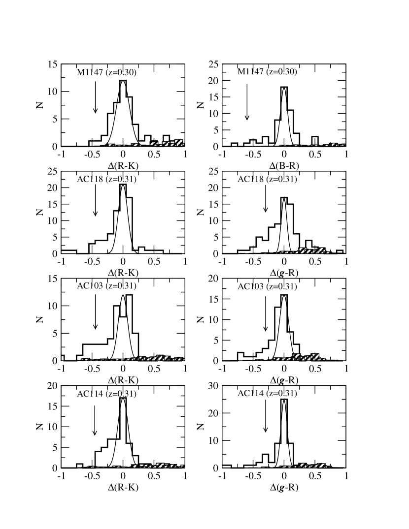
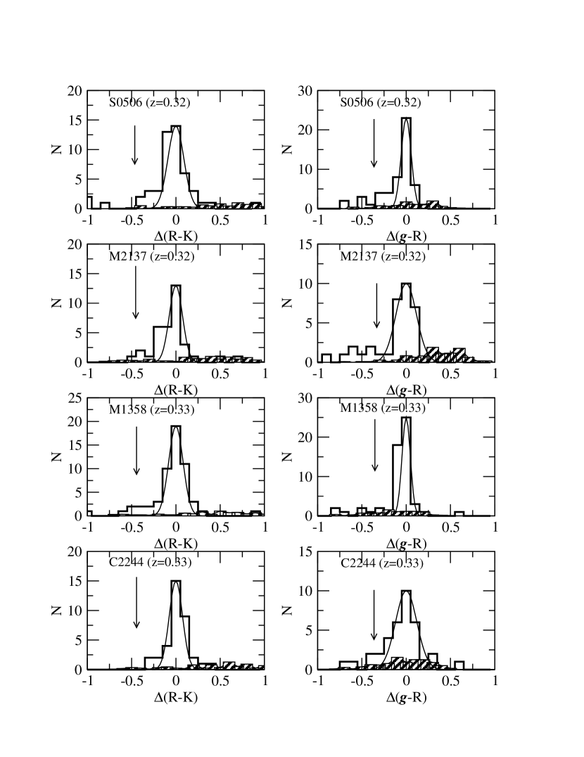
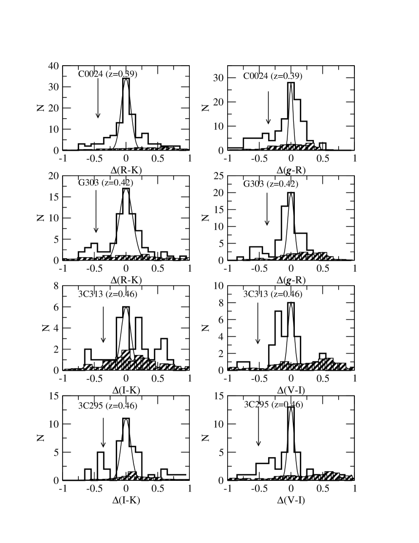
Figure 3: continued

Figure 3: continued

Figure 3: continued

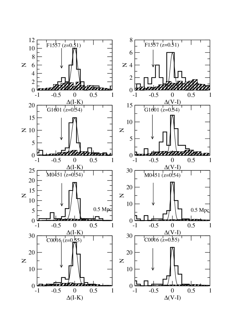
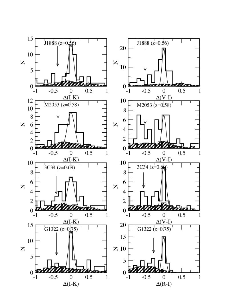
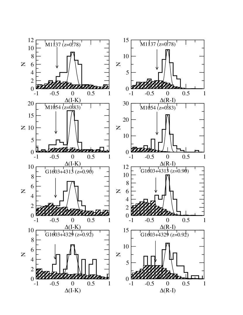
Figure 3: continued

The marginal color distributions for the clusters and the field sample, normalized by the relative areas and with the appropriate magnitude limits, are shown in Figure 3. The partial galaxies in the field histograms are due to the normalization to the area and magnitude limit of each cluster. As we state above, we have checked that the mode of the color distributions are close to 0 as expected. This does not always work perfectly both because measurement scatter in the colors tends to place fainter objects towards the red, and because field galaxies are in the color-magnitude diagrams biasing the fits to the cluster color-mag sequences. The distributions for M0906 are a special case: note they have modes which are significantly different from 0. This appears to be due to the fact that this cluster is composed of two clumps in redshift space, each with its own color-magnitude relation (Ellingson et al., 2001).

The arrow in each panel of Figure 3 indicates the color corresponding to $(B-V)_{rest}=$0.2 mag bluer than the early-type c–m relation. The blue fraction is defined as the ratio $N_{b}/N$, where $N_{b}$ is the field-corrected number of galaxies bluer than the BO84 color limit, and $N$ is the total number of cluster members (in a statistical sense, after subtraction of the field population). The error in this quantity is derived from

$${\sigma^{2}(f_{B})\over f_{B}^{2}}=\Big{(}{\sigma^{2}N_{b}\over N^{2}_{b}}\Big{)}+\Big{(}{\sigma^{2}N\over N^{2}}\Big{)}$$

and

$$N=N{\rm(all)}-N{\rm(field)}$$

$$N_{b}=N_{b}{\rm(all)}-N{\rm(field)}$$

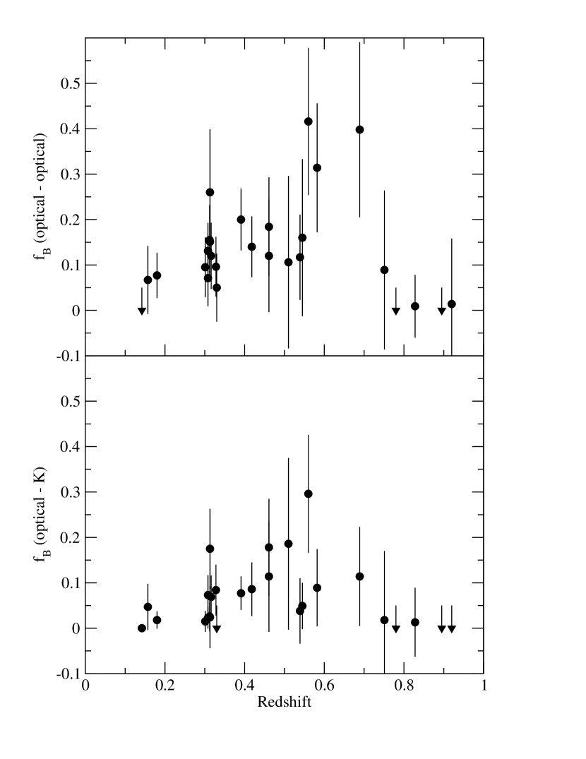
Figure 4: Variation of the blue fraction with redshift in the 0.7 Mpc fields in all clusters for both the optical$-K$ (bottom panel) and the optical color (top panel). The upper limits (downward pointing arrows) indicate clusters for which the derived f_B is negative because of overcorrection of the field population.

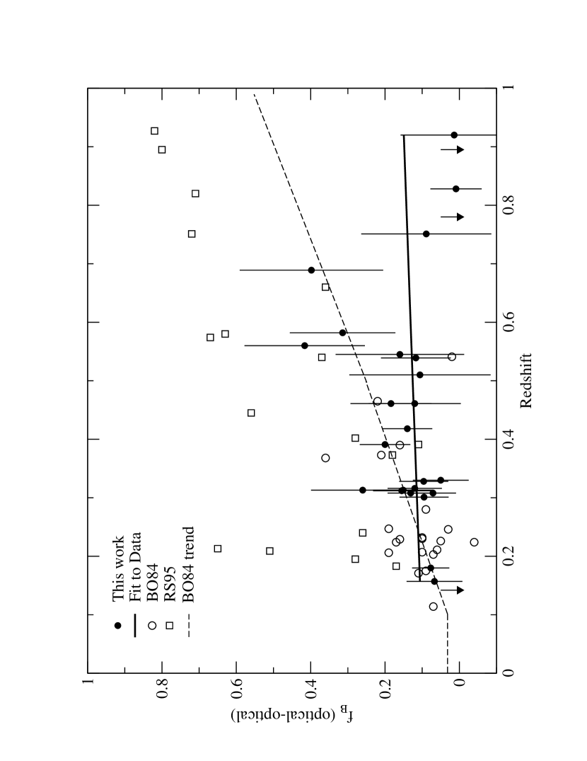
Figure 5: Comparison of blue fractions in our optical colors with BO84 and Rakos & Schombert (1995) for the R=0.7 Mpc fields. Closed symbols are our data; open circles show BO84’s and open squares Rakos & Schombert (1995)’s data. Upper limits as for Figure 4 above. The thick solid line is a linear fit to our data to show the trend in blue fraction with redshift. The thin dot dashed line is the fit shown by BO84 to their data, extrapolated to $z=1$.

where $N{\rm(all)}$ and $N_{\rm(field)}$ are Poisson variables (including an extra contribution from clustering which is computed from the four separate background fields of SPICES) and $N_{b}{\rm(all)}$ and $N_{b}{\rm(field)}$ are binomial variables. The correction for field contamination is statistical which means that the corrections can be too large resulting, on some occasions, in blue fractions that are negative. In these cases we have indicated that the value is an upper limit in Figures 4 and 5 below.

We plot blue fractions as a function of redshift for the 0.7 Mpc radii for both optical-infrared and optical-optical colors in Figure 4, and compare our results for the optical colors with the previous compilations by BO84 and Rakos & Schombert (1995) in Figure 5. The derived $f_{B}$’s for our $K$-selected samples are tabulated in Table 3. A fit to our data shows that $f_{B}$ is about 10% at all redshifts we consider (albeit with large scatter).

To see if there are any systematic differences between our blue fractions and those reported by BO84, we have attempted to make direct comparisons with BO84. For this purpose, there are four clusters in both our sample and that of BO84 for which we have adequate data to make useful comparisons: Abell 1942, CL0024+1654, 3C 295, and CL0016+16. For these clusters, we have selected samples in both the $K$-band and also in an optical band, $R$ or $I$, depending on the cluster redshift. Our samples are chosen over the same areas as in BO84, and to the same magnitude limits actually used by BO84, to the extent that these magnitude limits can be determined from the literature. The areas and magnitude limits for these comparisons are summarized, along with the resulting blue fractions, in Table 2. For 3 of the 4 clusters we find blue fractions in our optically-selected samples similar to those calculated by BO84. The exception is CL0016+16, the highest redshift cluster in BO84 at $z=0.54$, for which we determined a significantly higher value of $f_{B}$. However, the $f_{B}=0.02\pm 0.07$ found by BO84 is far below the value of $f_{B}$ predicted by the Butcher-Oemler effect for the cluster’s redshift. For all four clusters the $f_{B}$ that we found in our $K$-selected sample in this comparison are lower than those found from the optically-selected samples, even when the area and effective magnitude limits are the same. So these tests indicate that selecting in the $K$-band is the most important factor determining the generally lower values of $f_{B}$ that we find from our $K$-band selected samples.

4 Discussion

We find that: (i) our infrared selected blue fractions are generally lower than optically selected $f_{B}$ and (ii) our data show no strong trend in $f_{B}$ with redshift. However, at the redshifts $z<0.6$ where our sample overlaps with that of Butcher & Oemler, there is little if any significant difference in $f_{B}$ as determined from our $K$-selected samples and those of Butcher & Omeler, given the larger scatter in the $f_{B}$ found both by us and by Butcher & Oemler.

These points need further clarification. Our sample of clusters is heterogeneous and is somewhat biased to rich clusters at higher redshifts, for which blue fractions could be lower, as these objects are more likely to be more dynamically evolved. Andreon & Ettori (1999) show that the BO effect weakens when X-ray selected clusters are added to the set of clusters in BO84. However, we have shown that the same degree of passive evolution is present in at least the early-type galaxies in our sample (Stanford et al., 1998; De Propris et al., 1999) independent of the X-ray luminosity of the cluster.

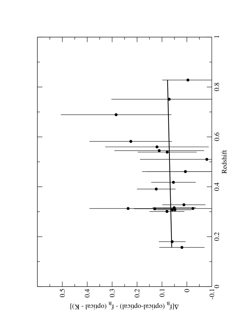
Figure 6: Differences in blue fractions between optical-only and $R/I-K$ colors as a function of redshift for the R=0.7 Mpc aperture. The thick solid line is a straight line fit to these differences.

The $K$-band selection procedure adopted will identify galaxies with colors of Sb’s or later types, as long as they are above our magnitude limit (i.e. are sufficiently massive). At the redshifts we are considering, the $R$ band passes through the rest frame $B$ and $U$ passbands, whereas $I$ samples the $V$ and $B$ bands, so our optical colors should be sensitive even to minor episodes of star formation in otherwise old populations. We show a comparison of blue fractions as derived in the optical-$K$ and optical-only colors in Figure 6. There is no evidence of large systematic differences in the derived blue fractions in these colors. On average the difference in blue fractions between optical-$K$ and purely optical colors is $0.07\pm 0.10$. Our $K$ selected sample is roughly equivalent to selection by stellar mass and therefore our results indicate that the star formation likely causing the BO effect takes place among relatively low mass objects as well as in normal spirals Dressler et al. (1994), Oemler et al. (1997).

A plausible interpretation of our results is that there are two components to the classical BO effect. One component, which is seen by our $K$-selected samples giving rise to the $\sim$10% values of $f_{B}$ that we find, is the massive galaxies, with colors approximately equivalent to those of Sb’s, that are present at a roughly constant fraction at all redshifts; these objects are likely to be field spirals whose star formation history is modified by infall into the cluster. The second component, which is missing from our infrared selected data, is responsible for both the larger blue fractions of optically-selected samples and their redshift dependence. If this is correct, these objects have $K-$band luminosities lower than $K^{*}+1.5$ and are likely to be a population of starbursting dwarfs (or low luminosity spirals), subject to luminosity boosting in the optical bands (Barger et al., 1996). The first population would be identified with the ‘normal’ spirals of C94 and C98, whereas the dwarfs would constitute the more extreme starburst and post-starburst objects. These dwarfs are unlikely to evolve into S0’s and instead contribute to the rich populations of dwarf galaxies observed in nearby clusters. As dwarfs are sampled from the more steeply rising power-law regime of the luminosity function ($\alpha\sim-1.3$), the exact placement of an optical magnitude limit with respect to $M^{\ast}$ strongly affects the number of dwarfs included in a sample and thus can result in a large increase in observed $f_{B}$. This is qualitatively consistent with the results of C98, where the greater part of the blue population corresponds to relatively low mass late type spirals and irregulars.

There is considerable evidence that low luminosity galaxies show greater star forming activity at moderate redshifts. The Canada-France Redshift Survey detected a population of bright objects with strong OII emission at $z>0.2$ (Hammer et al., 1997). The blue excess field population at $z=0.5$ consists of dwarfs (kinematically: Mallén-Ornelas et al. 1997). The luminosity function of dwarfs in two distant clusters, MS 2255.7+2039 at $z=0.29$ (Näslund et al., 2000) and CL1601+54 at $z=0.54$ (Dáhlen et al., 2001), appears to steepen with redshift, suggesting a brightening of the dwarf population associated with star formation episodes. Such objects would then fade to become part of the rich dwarf populations observed in nearby clusters (Wilson et al., 1997). This is consistent with the ‘harassment’ scenario of Moore et al. (1998) whereby low mass spirals are transformed into spheroidals via interactions with the cluster tidal field. A possible interpretation then would account for the Butcher-Oemler effect as a cluster counterpart of the faint blue field galaxies, coupled with an increase in cluster infall at larger redshift, as in the scenario presented by Ellingson et al. (2001).

Although our data only provide information on the bright, massive component of the BO effect, we observe that there is no redshift at which the blue fractions peak strongly in Figure 4. If the blue galaxies in our $K$-selected samples are mostly normal spirals falling into clusters, this suggests that there is no preferred epoch of cluster merging and that spiral and lenticular populations may be built up gradually by infall of small groups at least since $z\sim 1$.

To conclude, we need to caution the reader that our results are based on a heterogeneous sample of objects, which is likely to contain significant observational biases. One obvious example is that the fit in Fig. 5 is weighed to low blue fraction by the small number of clusters at $z>0.7$ which have low $f_{B}$. If we exclude these from our fit, we still find a shallower slope than BO84 but the discrepancy is much reduced. The higher redshift clusters are those most likely to be massive and to have low blue fractions because more highly evolved. This points to the the need to acquire more data, over wider fields of view and to fainter limits, and for a larger sample of clusters at high redshift, in order to confirm the results presented here.

Table 1: Reference magnitudes vs. $z$

Redshift	$K_{*}$	$K_{lim}$	$K(BO)$	actual $K(BO)$
0.15	$14.84\pm 0.49$	16.3	16.5	16.5
0.20	$15.16\pm 0.07$	16.7	17.0	17.0
0.25	$15.64\pm 0.38$	17.1	17.5	17.5
0.32	$15.74\pm 0.08$	17.2	18.0	18.0
0.40	$16.50\pm 0.11$	18.0	18.5	17.8
0.46	$16.38\pm 0.08$	17.9	18.8	17.7
0.54	$16.85\pm 0.18$	18.4	19.2	18.2
0.69	$17.2\tablenotemark{e}\pm 0.4$	18.7	19.1	$\cdots$
0.79	$17.51\pm 0.26$	19.0	20.1	$\cdots$
0.90	$18.05\pm 0.25$	19.5	20.4	$\cdots$

Table 2: Comparisons with BO84

Cluster	BO84 $f_{B}$	R(30)	BO84 limit	Nsample (BO84)	Optical $f_{B}$	IR $f_{B}$	radius	$K_{lim}$	Nfield/Nsample
		arcmin	$M(V)$				arcmin
Abell 1942	$0.17\pm 0.05$	2.8	-20.0	57	$0.21\pm 0.05$	$0.16\pm 0.04$	2.2	17.3	8.7/65
CL0024+16	$0.16\pm 0.02$	1.1	-20.8	87	$0.16\pm 0.02$	$0.08\pm 0.03$	1.1	17.8	5.7/76
3C 295	$0.23\pm 0.05$	1.0	-21.1	45	$0.27\pm 0.10$	$0.14\pm 0.04$	1.0	17.8	5.5/26
CL0016+16	$0.02\pm 0.07$	1.0	-21.0	65	$0.18\pm 0.06$	$0.09\pm 0.06$	1.0	18.3	9/51

Table 3: Blue Fractions for the complete cluster sample

Cluster ID	Redshift	$f_{B}(R/I-K)$	$f_{B}(R/I-K)$	$f_{B}$ (optical)	$f_{B}$ (optical)	$N_{field}/N_{sample}$	$N_{field}/N_{sample}$
		R=0.5 Mpc	R=0.7 Mpc	R=0.5 Mpc	R=0.7 Mpc	R=0.5 Mpc	R=0.7 Mpc
A1146	0.142	$0.000\pm 0.000$	$0.000\pm 0.000$	$-0.020\pm 0.044$	$-0.024\pm 0.046$	1.7/38	3.3/55
A3305	0.157	$0.050\pm 0.056$	$0.047\pm 0.051$	$0.038\pm 0.058$	$0.067\pm 0.075$	4.0/24	7.8/29
MS0906.5+1110	0.180	$0.027\pm 0.029$	$0.018\pm 0.019$	$0.029\pm 0.045$	$0.077\pm 0.050$	5.3/42	10.3/65
A1689	0.185	$0.046\pm 0.038$	$\cdots$	$0.029\pm 0.025$	$\cdots$	5.2/91	$\cdots$
A1942	0.224	$0.069\pm 0.053$	$\cdots$	$0.054\pm 0.051$	$\cdots$	3.8/47	$\cdots$
MS1253.9+0456	0.230	$0.090\pm 0.055$	$\cdots$	$0.112\pm 0.069$	$\cdots$	6.7/59	$\cdots$
A1525	0.259	$0.055\pm 0.048$	$\cdots$	$0.051\pm 0.061$	$\cdots$	5.7/40	$\cdots$
M1008-1225	0.301	$0.000\pm 0.010$	$0.015\pm 0.023$	$0.047\pm 0.054$	$0.085\pm 0.066$	5.2/44	10.4/60
M1147+1103	0.308	$0.036\pm 0.040$	$0.023\pm 0.024$	$0.112\pm 0.092$	$0.071\pm 0.062$	5.2/33	10.3/54
AC118	0.308	$0.073\pm 0.054$	$0.073\pm 0.044$	$0.123\pm 0.076$	$0.131\pm 0.062$	5.2/52	10.3/77
AC114	0.312	$0.050\pm 0.051$	$0.026\pm 0.033$	$0.148\pm 0.096$	$0.155\pm 0.077$	5.1/38	10.1/60
AC103	0.313	$0.107\pm 0.078$	$0.175\pm 0.088$	$0.082\pm 0.064$	$0.161\pm 0.088$	5.1/39	10.0/57
MS2137-0234	0.313	$0.014\pm 0.057$	$0.024\pm 0.068$	$0.177\pm 0.124$	$0.260\pm 0.139$	5.1/27	10.1/36
Abell S0506	0.316	$0.029\pm 0.034$	$0.069\pm 0.047$	$0.077\pm 0.066$	$0.120\pm 0.073$	5.0/38	9.8/52
M1358+6245	0.328	$0.046\pm 0.050$	$0.084\pm 0.056$	$0.054\pm 0.062$	$0.096\pm 0.056$	4.8/39	9.4/59
CL2244-02	0.330	$-0.014\pm 0.026$	$-0.022\pm 0.029$	$0.007\pm 0.061$	$0.050\pm 0.075$	4.8/26	9.4/36
CL0024+16	0.391	$0.081\pm 0.044$	$0.077\pm 0.037$	$0.153\pm 0.068$	$0.200\pm 0.068$	10.2/88	20/119
GHO 0303+1706	0.418	$0.065\pm 0.064$	$0.086\pm 0.059$	$0.174\pm 0.096$	$0.140\pm 0.067$	9.5/46	18.5/74
3C 313	0.461	$0.010\pm 0.112$	$0.114\pm 0.122$	$-0.070\pm 0.083$	$0.120\pm 0.124$	7.3/19	14.3/34
3C 295	0.461	$0.194\pm 0.134$	$0.178\pm 0.107$	$0.240\pm 0.152$	$0.184\pm 0.109$	7.3/29	14.4/45
F1557.19TC	0.510	$-0.021\pm 0.105$	$-0.186\pm 0.189$	$0.143\pm 0.132$	$0.106\pm 0.190$	10.6/29	20.7/34
GHO 1601+4253	0.539	$0.027\pm 0.077$	$0.038\pm 0.072$	$0.020\pm 0.078$	$0.117\pm 0.094$	10.1/33	19.8/53
MS0451.6-0306	0.539	$0.121\pm 0.066$	$\cdots$	$0.197\pm 0.089$	$\cdots$	10.1/70	$\cdots$
CL0016+16	0.545	$0.000\pm 0.043$	$0.049\pm 0.051$	$0.193\pm 0.098$	$0.160\pm 0.073$	10/52	19.5/80
J1888.16CL	0.560	$0.243\pm 0.142$	$0.296\pm 0.130$	$0.353\pm 0.181$	$0.416\pm 0.162$	9.7/36	19.1/59
MS2053-0449	0.582	$0.083\pm 0.116$	$0.089\pm 0.085$	$0.226\pm 0.168$	$0.314\pm 0.142$	9.4/30	18.4/58
3C 34	0.689	$-0.067\pm 0.092$	$0.114\pm 0.109$	$0.143\pm 0.153$	$0.398\pm 0.193$	9.3/28	18.1/47
GHO 1322+3027	0.751	$-0.180\pm 0.188$	$0.018\pm 0.152$	$-0.200\pm 0.231$	$0.089\pm 0.173$	12.9/26	25.2/49
MS1137.5+6625	0.780	$-0.006\pm 0.099$	$-0.040\pm 0.120$	$0.014\pm 0.121$	$-0.101\pm 0.137$	12.6/38	24.7/55
MS1054.5-0327	0.820	$0.052\pm 0.065$	$0.105\pm 0.057$	$0.013\pm 0.076$	$0.009\pm 0.069$	12.2/54	24.1/86
GHO 1603+4313	0.895	$-0.070\pm 0.191$	$-0.363\pm 0.361$	$-0.310\pm 0.236$	$-0.987\pm 0.653$	17.1/33	33.5/48
GHO 1603+4329	0.920	$-0.297\pm 0.393$	$-0.342\pm 0.251$	$0.050\pm 0.190$	$0.014\pm 0.144$	15.5/24	30.4/54

Figure 1: continued

Figure 1: continued

Figure 2: Comparison between interpolated and measured colors for galaxies in the SPICES survey.

Figure 3: continued

Figure 3: continued

References

- Abraham et al. (1996) Abraham, R. et al, 1996, ApJ, 471, 694
- Andreon & Ettori (1999) Andreon, S., & Ettori, S. 1999, ApJ, 516, 647
- Aragon-Salamanca et al. (1991) Aragon-Salamanca, A., Ellis, R. S. & Sharples, R. M. 1991, MNRAS, 248, 128
- Balogh et al. (2000) Balogh, M. L., Navarro, J. F., & Morris, S. L. 1999, ApJ, 527, 54
- Barger et al. (1996) Barger, A. J., Aragon-Salamanca, A., Ellis, R. S., Couch, W. J., Smail, I. & Sharples, R. M. 1996, MNRAS, 279, 1
- Butcher & Oemler (1978) Butcher, H., & Oemler, A. 1978, ApJ, 226, 559
- Butcher & Oemler (1984) Butcher, H., & Oemler, A. 1984, ApJ, 285, 426
- Coleman et al. (1980) Coleman, G. D., Wu, C.-C., & Weedman, D. W. 1980, ApJS, 43, 393
- Connolly & Szalay (1999) Connolly, A. J. & Szalay, A. S. 1999, AJ, 117, 2052
- Couch & Sharples (1987) Couch, W. J., & Sharples, R. M. 1987, MNRAS, 229, 483
- Couch et al. (1994) Couch, W. J., Ellis, R. S., Sharples, R. M. & Smail, I. 1994, ApJ, 430, 121
- Couch et al. (1998) Couch, W. J., Barger, A. J., Smail, I., Ellis, R. S. & Sharples, R. M. 1998, ApJ, 497, 188
- Csabai et al. (2000) Csabai, I., Connolly, A. J., Szalay, A. S. & Budávari, T. 2000, AJ, 119, 69
- Dáhlen et al. (2001) Dáhlen, T., Fransson, C. & Näslund, M. 2001, MNRAS, 330, 167
- De Propris et al. (1999) De Propris, R., Stanford, S. A., Eisenhardt, P. R., Dickinson, M., & Elston, R. 1999, AJ, 118, 719
- Dressler (1980) Dressler, A. 1980, ApJ, 236, 351
- Dressler & Gunn (1983) Dressler, A. & Gunn, J. E. 1983, ApJ, 270, 7
- Dressler et al. (1994) Dressler, A., Oemler, A., Butcher, H., & Gunn, J.E. 1994, ApJ, 430, 107
- Dressler et al. (1997) Dressler, A. et al. 1997, ApJ, 490, 577
- Eisenhardt et al. (2003) Eisenhardt, P. R., De Propris, R., Gonzales, A., Stanford, S. A., Dickinson, M. & Wang, M., in preparation
- Eisenhardt et al. (2003) Eisenhardt, P. R., Elston, R., Stanford, S. A., Stern, D., Wu, K. L., Connolly, A. J. & Spinrad, H. 2003, in preparation
- Ellingson et al. (2001) Ellingson E., Lin H., Yee H. K. C. & Carlberg R. 2001, ApJ, 547, 609
- Gavazzi et al. (1996) Gavazzi, G., Pierini, A. & Boselli, D. 1996, A&A, 312, 297
- Hammer et al. (1997) Hammer, F. et al. 1997, ApJ, 481, 49
- Kauffmann (1995) Kauffmann, G. 1995, MNRAS, 274, 161
- Koo (1981) Koo, D. 1981, ApJ, 251, L75
- Larson et al. (1980) Larson, R. B., Tinsley, B. M. & Caldwell, C. N. 1980, ApJ, 237, 692
- Lavery & Henry (1988) Lavery, R. J., & Henry, J. P. 1988, ApJ, 330, 596
- Mallén-Ornelas et al. (1999) Mallén-Ornelas, G., Lilly, S. J., Crampton, D. & Schade, D. 1999, ApJ, 518, L83
- Margoniner & de Carvalho (2000) Margoniner, V. E., & de Carvalho, R. R. 2000, AJ, 119, 1562
- Margoniner et al. (2001) Margoniner, V.E., De Carvalho, R.R., Gal, R., & Djorgovski, S.G. 2001, ApJ, 548, L143
- Metevier et al. (2000) Metevier, A. J., Romer, A. K. & Ulmer, M. P. 2000, AJ, 119, 1090
- Moore et al. (1998) Moore, B., Lake, G., & Katz, N. 1998, ApJ, 495, 139
- Morris et al (1998) Morris, S. L., Hutchings J. B., Carlberg, R. G., Yee, H. K. C., Ellingson, E., Balogh, M. L., Abraham, R. G., Smecker-Hane, T. A. 1998, ApJ, 507, 84
- Näslund et al. (2000) Näslund, M., Fransson, C., & Huldtgren, M. 2000, A&A, 356, 435
- Oemler et al. (1997) Oemler, A., Dressler, A. & Butcher, H. 1997, ApJ, 474, 561
- Poggianti (1997) Poggianti, B. M. 1997, A&AS, 122, 399
- Poggianti et al. (1999) Poggianti, B, M., Smail, I., Dressler, A., Couch, W. J., Barger, A. J.,Butcher, H., Ellis, R. S. & Oemler, A. 1999, ApJ, 578, 516
- Rakos & Schombert (1995) Rakos, K. D., & Schombert, J. M. 1995, ApJ, 439, 47
- Rakos et al. (1997) Rakos, K. D., Odell, A. D. & Schombert, J. M. 1997, ApJ, 490, 194
- Sandage & Visvanathan (1978) Sandage, A. & Visvanathan, N. 1978, ApJ, 223, 707
- Smail et al. (1998) Smail, I., Edge, A. C., Ellis, R. S. & Blandford, R. D. 1998, MNRAS, 293, 124
- Stanford et al. (1998) Stanford, S. A., Eisenhardt, P. R., & Dickinson, M. 1998, ApJ, 492, 461
- Stanford et al. (2002) Stanford, S. A., Eisenhardt, P. R., Dickinson, M., Holden, B. P., & De Propris, R. 2002, ApJS, 142, 153
- Stern et al. (2002) Stern, D. et al. 2002, AJ, 123, 2223
- Wilson et al. (1997) Wilson, G., Smail, I., Ellis, R. S., & Couch, W. J. 1997, MNRAS, 284, 915