Models for Type I X-Ray Bursts with Improved Nuclear Physics

Abstract

Multi-zone models of Type I X-ray bursts are presented that use an adaptive nuclear reaction network of unprecedented size, up to 1300 isotopes, for energy generation and include the most recent measurements and estimates of critical nuclear physics. Convection and radiation transport are included in calculations that carefully follow the changing composition in the accreted layer, both during the bursts themselves and in their ashes. Sequences of bursts, up to 15 in one case, are followed for two choices of accretion rate and metallicity, up to the point where quasi-steady state is achieved. For ${\dot{M}}=1.75{{\times}{10^{-9}}}\,{{\mathrm{M}_{\odot}}\,{\mathrm{yr}}^{-1}}$ (and ${\dot{M}}=3.5{{\times}{10^{-10}}}\,{{\mathrm{M}_{\odot}}\,{\mathrm{yr}}^{-1}}$, for low metallicity), combined hydrogen-helium flashes occur. These bursts have light curves with slow rise times (seconds) and long tails. The rise times, shapes, and tails of these light curves are sensitive to the efficiency of nuclear burning at various waiting points along the rp-process path and these sensitivities are explored. Each displays “compositional inertia” in that its properties are sensitive to the fact that accretion occurs onto the ashes of previous bursts which contain left-over hydrogen, helium and CNO nuclei. This acts to reduce the sensitivity of burst properties to metallicity. Only the first anomalous burst in one model produces nuclei as heavy as $A=100$. For the present choice of nuclear physics and accretion rates, other bursts and models make chiefly nuclei with $A\approx 64$. The amount of carbon remaining after hydrogen-helium bursts is typically $\lesssim 1$% by mass, and decreases further as the ashes are periodically heated by subsequent bursts. For ${\dot{M}}=3.5{{\times}{10^{-10}}}\,{{\mathrm{M}_{\odot}}\,{\mathrm{yr}}^{-1}}$ and solar metallicity, bursts are ignited in a hydrogen-free helium layer. At the base of this layer, up to 90% of the helium has already burned to carbon prior to the unstable ignition of the helium shell. These helium-ignited bursts have a) briefer, brighter light curves with shorter tails; b) very rapid rise times ($<0.1\,$s); and c) ashes lighter than the iron group.

1. Introduction

Since the 1970’s, when the nuclear instability of accretion onto neutron stars was noted (Hansen & van Horn, 1975), and the connection with short, transient X-ray flashes (Type I X-ray bursts) pointed out (Woosley & Taam, 1976), there have been numerous studies of thermonuclear flashes on neutron stars. For reviews, see Lewin et al. 1993, 1995; Bildsten 1998; Strohmayer & Bildsten 2003. Studies in the mid-1980’s elucidated the relevant nuclear physics, known as the rp-process (Wallace & Woosley, 1981), and showed that the most critical parameter determining burst properties was the accretion rate, with several different regimes of bursting behavior expected (Fujimoto et al., 1981; Fushiki & Lamb, 1987). In particular, combined helium and hydrogen burning powers flashes with the lowest critical masses for accretion rates between $4$–$11{{\times}{10^{-10}}}$ and $2{{\times}{10^{-8}}}$ ${{\mathrm{M}_{\odot}}\,{\mathrm{yr}}^{-1}}$ (depending upon the metallicity of the accreted matter), whereas pure helium flashes occur beneath a stable hydrogen shell for rates between $2{{\times}{10^{-10}}}$ and $4$–$11{{\times}{10^{-10}}}\,{{\mathrm{M}_{\odot}}\,{\mathrm{yr}}^{-1}}$. Weakly flashing hydrogen shells occur for rates less than $2{{\times}{10^{-10}}},{{\mathrm{M}_{\odot}}\,{\mathrm{yr}}^{-1}}$. The generic properties predicted for these flashes — intervals, durations, energies, brightness, etc. — were in good agreement with observations, though the trends in burst properties with changing accretion rate were often at odds with the simple theory (e.g., van Paradijs et al. 1988; Bildsten 2000).

Previous theoretical studies can generally be criticized, however, either for oversimplification of the nuclear physics, especially the use of small approximation networks for the energy generation, e.g., Taam 1980; Ayasli & Joss 1982; Woosley & Weaver 1984, or for inadequate attention to the stellar model, especially convection, in single-zoned studies that use large reaction networks (Schatz et al., 2001a, b; Brown et al., 2002). In this paper, we combine both: large networks and current nuclear data with leading edge (albeit one-dimensional) stellar models that include convection and multi-zone radiation transport.

Any such attempt to simulate Type I X-ray bursts realistically meets with four challenges. First is the physics of the accretion process and the geometry of the runaway. Is the accretion uniformly distributed over the surface of the neutron star prior to runaway and does the burst commence almost simultaneously over that surface? Observations of nearly-coherent oscillations during Type I bursts in the last six years have brought these questions into focus (see Strohmayer & Bildsten 2003 for a review). The oscillations, which are interpreted as rotational modulation of brightness asymmetries, indicate rapid rotation, and perhaps non-uniform ignition. If so, rotation may be key to balancing the strong transverse pressure gradients that arise near a local hot spot (Spitkovsky et al., 2002; Zingale et al., 2003). We do not address these issues in this paper; our one-dimensional calculations address only the local physics per unit area. While comparison to observables like the light curve could be affected by the geometry, the nuclear physics of the runaway is not.

Second, the nuclear physics is complex with no single or even several reactions governing the energy generation rate. Recent years have brought significant advances in our understanding of the major flows in the rp- and $\alpha$p-processes and the properties of the nuclei that govern them (e.g., Schatz et al. 2001a, b; Brown et al. 2002). These advances should be included in any modern study.

A particularly exciting development has been the discovery of very energetic, long duration Type I bursts, known as “superbursts” (see Kuulkers et al. 2002 for a review of superburst properties). These flashes have 1000 times the energy and duration of normal Type I bursts, and have been interpreted as unstable ignition of a thick carbon layer (Cumming & Bildsten, 2001; Strohmayer & Brown, 2002), originally proposed by Woosley & Taam (1976) as a gamma-ray burst model. Calculating the amount of carbon produced during unstable hydrogen/helium burning, and how much carbon survives to great depth, requires an accurate multi-zone calculation with a large nuclear network.

The third challenge is following not just one, but many bursts. As was pointed out by Taam (1980), the thermal and compositional “inertia” of the neutron star envelope can have important implications for the properties of subsequent bursts. It is only by computing a succession of X-ray bursts that the heating associated with the previous thermonuclear flashes and compositional change in the accreted layer can be taken into account (Ayasli & Joss, 1982; Woosley & Weaver, 1984; Taam et al., 1993). Here we not only carry out fine-zoned studies of individual bursts, but follow each case until a steady state is achieved, including in one study, 15 consecutive bursts.

The fourth challenge is making contact with the rich archive of photometry and spectra for observed X-ray bursts. The models presented here are limited to single-temperature black bodies calculated using flux-limited radiative diffusion, although more detailed studies of the spectrum and color temperature could use our results as input to a more superior treatment of radiation transport. An immediate application of our results is direct comparisons with observed light curves to study, for example, the physics underlying burst rise and decay times. We do not attempt such a comparison in this initial paper, but leave this for future work.

An outline of the paper is as follows. In § 2 we describe modifications to the one-dimensional implicit hydrodynamics code – Kepler – used for this study. This code has been used before to study X-ray bursts (e.g., Woosley & Weaver 1984; Fushiki et al. 1992; Taam et al. 1993, 1996) and we need only clarify recent modifications to the nuclear reaction library and the implementation of energy generation from an extended network. A novel approach to evolving the abundance vector in each zone, called an “adaptive reaction network”, is employed in which the number of isotopes employed in each cycle of each stellar model may vary according to the active flows and significant abundances present. At maximum, we employed over 1300 isotopes in the reaction network for over 1000 zones at a time. The energy generation obtained from this network is used in calculating the stellar model.

In subsequent sections we describe the results for four models that crudely sample the accretion rates and compositions relevant for X-ray bursts. Two accretion rates, $3.5$ and $17.5{{\times}{10^{-10}}}\,{{\mathrm{M}_{\odot}}\,{\mathrm{yr}}^{-1}}$ and two metallicities, $Z=0.001$ and $0.02$ are examined. As expected, in three of these combined hydrogen helium runaways were observed. In the fourth, $Z=0.02$ and ${\dot{M}}=3.5{{\times}{10^{-10}}}\,{{\mathrm{M}_{\odot}}\,{\mathrm{yr}}^{-1}}$, hydrogen burns away before helium ignites in a thick shell that has already burned, at its base, mostly to carbon.

In the results and conclusions sections we describe some of the novel aspects of our results, the sensitivity to nuclear rates employed, the light curves and intervals for the bursts, and the composition of the ashes after many bursts have occurred, addressing both the expected composition of the crust, and whether enough carbon is produced to power a superburst.

2. The Kepler Code and the Nuclear Data Employed

Kepler is a one-dimensional implicit hydrodynamics code adapted to the study of stellar evolution and explosive astrophysical phenomena (Weaver et al., 1978). It has been used for twenty years to simulate X-ray bursts on neutron stars. The equation of state allows for a general mixture of radiation, ions, and electrons of arbitrary degeneracy and relativity. Electron-positron pair formation is also accurately included. Convective mixing is modeled using mixing length theory in a time-dependent manner. That is, the composition is diffusively mixed with a diffusion coefficient calculated from the convective velocity. The convective criterion is Ledoux but with a substantial semi-convective diffusion coefficient, about $10\,\%$ of the radiative diffusion coefficient, in regions that are stable by the Ledoux criterion and unstable by Schwarzschild. A relatively small amount of convective overshoot is included by flagging convective boundary zones as semi-convective. The opacity, neutrino losses, and other aspects of the code have been discussed in Woosley et al. (2002). In particular, the recent OPAL and Los Alamos opacity tables are used wherever the helium mass fraction exceeds $10^{-5}$ and the temperature is less than ${10^{9}}\,{\mathrm{K}}$.

Accretion is handled as in Woosley & Weaver (1984) and Taam et al. (1996). In the Lagrangian code, the outer boundary pressure is increased to simulate the weight of the accreted matter at the given gravitational potential. This continues until the pressure equivalent to the mass of a new zone has accumulated. At that point a new zone is added to the grid with conditions like those in the previous outer zone. The surface boundary pressure is zeroed and the process begun anew. All runs accrete zones of $2{{\times}{10^{19}}}\,{\mathrm{g}}$ and all accreted zones are retained until the end of the run, i.e., there was no re-zoning of the accreted layers. Some models accumulated more than 1000 zones this way. Typically, the zones at the base of the accreted layer become significantly thinner than $1\,{\mathrm{cm}}$!

During the accretion process, nuclear energy generation and composition change are calculated at every time step. Convection is always “on” in the sense that, if the Ledoux criterion for instability is satisfied, the code responds. In this way we found that, even though the strongest convection accompanied the onset of a burst, there were interesting episodes of both convection and thermohaline mixing in between the bursts.

2.1. Adaptive network

The major improvement in the present study was a more detailed treatment of the nuclear physics and energy generation. Unlike previous multi-zone calculations that carried only a very sparse “approximation network”, we computed energy generation and composition changes with a much larger network previously used only to study nucleosynthesis.

Reaction rates were extracted from a library of nuclear data (§ 2.3) carried in the calculation for isotopes ranging from hydrogen to polonium ($Z=1$ to $84$). When the abundance of an isotope exceeded a threshold mass fraction of $10^{-17}$, all neighboring isotopes that could be accessed by (${{\mathrm{}}}{{\mathrm{}}}{\mathrm{n}}$,$\gamma$), (${{\mathrm{}}}{{\mathrm{}}}{\mathrm{p}}$,$\gamma$), ($\alpha$,$\gamma$), ($\alpha$,${{\mathrm{}}}{{\mathrm{}}}{\mathrm{n}}$), ($\alpha$,${{\mathrm{}}}{{\mathrm{}}}{\mathrm{p}}$), or (${{\mathrm{}}}{{\mathrm{}}}{\mathrm{p}}$,${{\mathrm{}}}{{\mathrm{}}}{\mathrm{n}}$) reactions and their inverse, as well as (2${{\mathrm{}}}{{\mathrm{}}}{\mathrm{p}}$,$\gamma$) were added. For (${{\mathrm{}}}{{\mathrm{}}}{\mathrm{n}}$,$\gamma$) and ($\gamma$,${{\mathrm{}}}{{\mathrm{}}}{\mathrm{n}}$) links the limit is somewhat smaller, $10^{-18}$. Additionally, all possible decays, ($e^{-},\nu_{\rm e}$), ($e^{+}$$\nu_{{{{{{\mathrm{}}}{{\mathrm{}}}{\mathrm{e}}}}}}$), ($e^{-}$$\bar{\nu}_{{{{{{\mathrm{}}}{{\mathrm{}}}{\mathrm{e}}}}}}$), and ($\alpha$), were included for all isotopes in the network independent of their abundance. Conversely, when the mass fraction of an isotope dropped below $10^{-23}$, and its presence is not necessary to satisfy any of the above conditions for adding it, it was removed from the network. These criteria were applied in all zones during each stage of the calculation and only one network, the sum of all these local conditions, was used at any point in time throughout the star. This is necessary since zones may mix at unpredictable times and locations during the evolution.

2.2. Binding energies

Nuclear flow through the rp-process waiting point nuclei is exponentially sensitive to the proton separation energies ($S_{p}$) of a few nuclei near the proton-drip line. Experimental values for the binding energies were taken from Audi & Wapstra (1995; AW95) where available (Fig. 1). For many of the relevant nuclei however, no experimental information is available and one must rely on theoretical mass predictions. For nuclei with $Z>N$ in the mass range $A=41$–$75$, we used the compilation of Brown et al. (2002), in which the experimentally determined masses of $N>Z$ nuclei, together with a Skyrme Hartree-Fock calculation of Coulomb displacement energies, are used to estimate masses for the $Z>N$ mirrors. These mass predictions have an uncertainty of about 100 keV for the mass difference to the mirror nucleus. This results in an average uncertainty of the proton separation energies of about $140\,{\mathrm{keV}}$ if the mirror masses are sufficiently well known. As Table 1 shows, for many of the relevant rp-process nuclei this is not the case and uncertainties are substantially larger, though still within a few hundred $\mathrm{keV}$.

For another large set of nuclei, we used the unpublished calculations of (Brown, 2002) (Fig. 1). These are obtained using the same displacement energy method as in Brown et al. (2002), but the theoretical error in the displacement energy is larger than 100 keV (though still within a few 100 keV) because of the need to apply a spherical basis to a mass region where some nuclei are strongly deformed. Furthermore, for many of these heavier nuclei, the masses of the $N>Z$ mirrors are not known experimentally. We then used the theoretical extrapolations of AW95 as a basis for the displacement energy method. The errors in the AW95 extrapolations for $A>76$ introduced an additional error of order 500 keV for nuclei near the Z = N line. When no information is available either from AW95 or Brown, we employed the theoretical estimates of Möller et al. (1995).

Table 1 shows the proton separation energies of several key nuclei important in determining flow past the waiting point nuclei with long half-lives against positron decay – ${{\mathrm{}}}{{\mathrm{{}^{64}}}}{\mathrm{Ge}}$, ${{\mathrm{}}}{{\mathrm{{}^{68}}}}{\mathrm{Se}}$, ${{\mathrm{}}}{{\mathrm{{}^{72}}}}{\mathrm{Kr}}$, and ${{\mathrm{}}}{{\mathrm{{}^{76}}}}{\mathrm{Sr}}$. As discussed by Ormand (1997) and Brown et al. (2002), uncertainties in the masses of ${{\mathrm{}}}{{\mathrm{{}^{64}}}}{\mathrm{Ge}}$ and ${{\mathrm{}}}{{\mathrm{{}^{68}}}}{\mathrm{Se}}$ dominate uncertainties in the proton separation energies of ${{\mathrm{}}}{{\mathrm{{}^{65}}}}{\mathrm{As}}$ and ${{\mathrm{}}}{{\mathrm{{}^{69}}}}{\mathrm{Br}}$, key nuclei in the rp-process.

2.3. Reaction rates

Nuclear reaction rates were taken from experiment, shell-model calculations, and statistical model (Hauser-Feshbach) calculations. An experimentally determined rate was adopted whenever possible. Largely, though, experimental information was unavailable for the proton-rich nuclei important in X-ray bursts. For nuclei in the mass range $A=44$–$63$, experimentally-undetermined (${{\mathrm{}}}{{\mathrm{}}}{\mathrm{p}}$,$\gamma$) rates were taken from the shell model calculations of Fisker et al. (2001). Those authors also provide a critical discussion of uncertainties inherent in the different methods of calculating rates near the proton drip line. All other reaction rates were calculated using the Hauser-Feshbach code Non-Smoker as described by Rauscher & Thielemann (2000).

2.4. Weak rates

Our calculations include electron capture

$$e^{-}+{{{{\mathrm{}}}{{\mathrm{{}^{A}}}}{\mathrm{Z}}}}\rightarrow{{{{\mathrm{}}}{{\mathrm{{}^{A}}}}{\mathrm{(Z-1)}}}}+{\nu_{{{{{{\mathrm{}}}{{\mathrm{}}}{\mathrm{e}}}}}}},$$ (1)

nuclear ${e^{+}}$ decay (positron emission)

$${{{{\mathrm{}}}{{\mathrm{{}^{A}}}}{\mathrm{Z}}}}\rightarrow{{{{\mathrm{}}}{{\mathrm{{}^{A}}}}{\mathrm{(Z-1)}}}}+e^{+}+{\nu_{{{{{{\mathrm{}}}{{\mathrm{}}}{\mathrm{e}}}}}}},$$ (2)

and the neutrino energy loss rates associated with the above processes. For low temperature and density ($T_{9}<0.5$, $\rho{Y_{e}}<10^{5}\,{\mathrm{g}\,\mathrm{cm}^{-3}}$), we adopt the ground state rates. This is appropriate for the proton rich nuclei of interest during rp-process burning. These nuclei have decays characterized by large Q-values, for which positron emission dominates over electron capture. We take ground state weak decay rates from experiment where available and from the compilation of Möller et al. (1997) otherwise. Möller et al. (1997) calculated weak decay assuming only the presence of Gamow-Teller (GT) transitions. As is discussed below, Fermi transitions dominate the lifetimes of many near-proton-drip line nuclei. For such nuclei the lifetime is typically a factor of $4$–$6$ shorter than that estimated from a consideration of GT transitions alone. This issue and others relating to the weak physics of $N\sim Z$ nuclei will be addressed in a future study.

For nuclei with $A\leq 60$ and for higher temperature and density ($T_{9}>0.5$, $\rho{Y_{e}}>10^{5}\,{\mathrm{g}\,\mathrm{cm}^{-3}}$), we include the influence on the weak rates of thermal population of excited states as well as continuum electron capture. These rates are taken from the compilation of Langanke & Martinez-Pinedo (2000, LMP), and from the compilation of Fuller et al. (1982, FFN) for nuclei not studied by Langanke & Martinez-Pinedo. With the exception of a slightly different interpolation of neutrino energy loss rates, interpolation of the weak rates is done following the prescription of Fuller et al. (1985).

Thermal effects on weak rates for near-proton-drip line nuclei in the mass range $A\sim 60$–$100$ follow simple systematics. Consideration of these systematics can be used to determine if our use of ground state lifetimes for these nuclei is reasonable. Fig. 2 illustrates important nuclear and weak flows near the waiting point nucleus ${{\mathrm{}}}{{\mathrm{{}^{72}}}}{\mathrm{Kr}}$. These flows are typical of those near the other waiting point nuclei in this mass region.

As can be seen from Fig. 2, important weak decay parents fall into four categories. Nuclei with $Z=N+1$ undergo $e^{+}$-decay to their isospin mirrors. For these nuclei, the ground state of the ($e^{+}$) daughter is the isobaric analog state (IAS) of the parent ground state, the first excited state of the daughter is the IAS of the first excited state in the parent, and so on for all of the levels. Because the nuclear Hamiltonian commutes with the isospin raising and lowering operators, the Q-values and rates for all of these (parent level)$\rightarrow$(IAS in daughter) Fermi transitions are approximately the same. GT transitions are not expected to dominate the decay rates because the GT strength is typically spread out over a wide range in daughter excitation energy. In addition, electron capture cannot compete with these large Q-value $\beta^{+}$ decays at the small temperatures and electron Fermi energies achieved in X-ray bursts. Consequently, the decay rates of $Z=N+1$ nuclei are essentially temperature and density independent (for the range of conditions found in X-ray bursts). For nuclei with $Z=N+2=$ even, the situation is similar. Each parent state decays via a Fermi transition to an IAS in the daughter and the decay rates for these nuclei are well approximated by the ground state decay rate.

Nuclei with $N=Z=$ odd also decay principally via Fermi transitions. However, while for these nuclei it is true that every low-lying daughter state has a low-lying IAS in the parent, the converse is not true. Parent states in these $N=Z=$ odd nuclei that do not decay via a Fermi transition typically decay about an order of magnitude slower than do states with a low lying IAS in the even-even daughter. Consequently, $e^{+}$-rates for these nuclei are approximately proportional to $G_{\mathrm{daughter}}/G_{\mathrm{parent}}$ (Pruet & Fuller, 2002). Here $G$ is the partition function and the ratio is a rapidly decreasing function of temperature because of the high level density of odd-odd nuclei (relative to even-even nuclei).

The last, and most important, class of $Z\sim N$ nuclei are those with $Z=N=$ even. Of these, only two have partition functions at $T_{9}=1.5$ (${{\mathrm{}}}{{\mathrm{{}^{76}}}}{\mathrm{Sr}}$ with $G\approx 1.7$ and ${{\mathrm{}}}{{\mathrm{{}^{80}}}}{\mathrm{Zr}}$ with $G\approx 1.6$) large enough for the decay of excited states to determine the lifetime (see also Schatz et al. (1998) for a discussion of $2^{+}$ lifetimes in X-ray bursts and estimates of $2^{+}$ excitation energies for $Z>82$ nuclei). For these two nuclei the thermal decay rate may be larger by a factor of $\sim 2-3$ than the ground state decay rate, though a more reasonable estimate is probably in the $30\,\%$ range. As with the other important decays, electron capture is negligible for $N=Z=$ even nuclei during rp-process burning.

Detailed calculations of thermal effects on the weak decays of $A>60$ nuclei should eventually be incorporated into X-ray burst studies. However, the above considerations suggest that the adoption of laboratory ground state rates is not too bad. One shortcoming of our procedure concerns $N=Z=$ odd nuclei. We typically underestimate the lifetime of these nuclei in the X-ray burst environment by about a factor of 5. For $A<80$ this error is not expected to be important because so little of the nuclear flow ($\sim 1\,\%$ or less) proceeds through the $e^{+}$-decay of these nuclei. With increasing atomic mass number the proton drip line tends closer to $N=Z$. Errors in the lifetimes of $N=Z=$ odd nuclei may have a larger influence on nuclear flow for $A>80$. However, a qualitative change in the flow is unlikely because the typical lifetimes of important $A>80$ nuclei are so short ($\sim 1\,{\mathrm{s}}$) compared to lifetimes of long-lived waiting point nuclei ($\approx 64\,{\mathrm{s}}$ for ${{\mathrm{}}}{{\mathrm{{}^{64}}}}{\mathrm{Ge}}$).

2.5. Neutrino Losses from Radioactive Decays

Neutrino losses during weak decays are an important part of the total energy budget, since neutrinos typically carry away a sizeable fraction (half or more) of the energy available in a decay. When a weak decay rate is estimated from the compilation of LMP or FFN, we also adopt the LMP or FFN value for the neutrino energy loss rate associated with that decay. For a few light nuclei (${{\mathrm{}}}{{\mathrm{{}^{7}}}}{\mathrm{Be}}$, ${{\mathrm{}}}{{\mathrm{{}^{13}}}}{\mathrm{N}}$, ${{\mathrm{}}}{{\mathrm{{}^{14,15}}}}{\mathrm{O}}$, ${{\mathrm{}}}{{\mathrm{{}^{17,18}}}}{\mathrm{F}}$), neutrino energy loss rates are calculated using experimentally determined ground state weak strength distributions. Other neutrino energy loss rates were estimated using a code provided to us by Petr Vogel. This code uses an empirical form of the GT⁺ strength distribution to estimate the average energy of neutrinos emitted in a decay. The neutrino energy loss rate is then taken to be the product of the weak decay rate and the average neutrino energy. Though empirical strength distributions cannot reliably reproduce ground state decay rates, they can do a fair job of estimating average neutrino energies because phase space so heavily favors those transitions with the most energetic outgoing neutrinos. For decays characterized by large Q-values, Vogel’s estimates of average neutrino energies typically agree with more detailed estimates (FFN, LMP) to within $10\,\%$ or $15\,\%$.

3. Initial Models and Setup

Four different combinations of accretion rate and metallicity were examined (Table 2). The first model, zM, employs conditions very similar to Schatz et al. (2001a): an accretion rate of $0.1\,{\dot{M}_{\mathrm{Edd}}}=8.8{{\times}{10^{3}}}\,{\mathrm{g}\,\mathrm{cm}^{-2}\,\mathrm{s}^{-1}}=1.75{{\times}{10^{-9}}}\,{{\mathrm{M}_{\odot}}\,{\mathrm{yr}}^{-1}}$ for a $10\,{\mathrm{km}}$  radius neutron star. For comparison, we also calculated a similar model, zm, with an accretion rate one-fifth as large. The composition in both cases was taken to be $75.9\,\%$ hydrogen, $24\,\%$ helium, and $0.1\,\%$ ${{\mathrm{}}}{{\mathrm{{}^{14}}}}{\mathrm{N}}$ by mass, corresponding approximately to the $Z={10^{-3}}$ used by Schatz et al.. Hereafter this is referred to as the $5\,\%$ solar composition, since the total mass fractions of CNO in the sun are about $20$ times larger. For comparison, we also calculated similar models ZM and Zm with solar metallicity ($70.48\,\%$ ${{\mathrm{}}}{{\mathrm{{}^{1}}}}{\mathrm{H}}$, $27.52\,\%$ ${{\mathrm{}}}{{\mathrm{{}^{4}}}}{\mathrm{He}}$, $2\,\%$ ${{\mathrm{}}}{{\mathrm{{}^{14}}}}{\mathrm{N}}$) and high and low accretion rates respectively. These are similar to the Anders & Grevesse (1989) solar abundances, but the rearrangement of the CNO isotopes into nitrogen that naturally occurs in the CNO cycle was skipped since this will occur rapidly at the high temperatures of the accretion process and the energy added is inconsequential compared with that of accretion.

To save time and improve energy conservation, only the outer $2{{\times}{10^{25}}}\,{\mathrm{g}}$ of neutron star crust is carried in the calculation. This is orders of magnitude larger than the mass of all X-ray bursts combined, so the layer essentially acts as a large repository of thermal inertia. Its composition is taken to be iron and no nuclear reactions are followed in this layer. We take the luminosity at the base of the substrate to be $3.2{{\times}{10^{33}}}\,{\mathrm{erg}\,\mathrm{s}^{-1}}$ for Models zm and Zm and $1.6{{\times}{10^{34}}}\,{\mathrm{erg}\,\mathrm{s}^{-1}}$ for Models zM and ZM, i.e., the accretion rate times $0.15\,{\mathrm{MeV}}$/nucleon as in Schatz et al.. Before accretion is switched on, we allow the substrate to relax to thermal steady state with the power input at its base balanced by the luminosity flowing into the accreted zones.

A $1.4\,{\mathrm{M}_{\odot}}$ neutron star with radius $R=10\,{\mathrm{km}}$ is adopted giving a surface gravity $g=GM/R^{2}=1.9{{\times}{10^{14}}}\,{\mathrm{cm}^{-2}\,\mathrm{s}^{-1}}$. We do not include the effects of general relativity in our simulations, we address the relativistic corrections that must be applied to our results in § 4.4.

4. Results

4.1. Model zM

The model considered in greatest detail and followed though the largest number of flashes was Model zM, whose parameters duplicated those of previous studies by Schatz et al. (2001a, b). The accretion rate and metallicity (Table 2) imply that hydrogen will survive to the depth where helium ignites, so that this should be a representative case of a combined hydrogen-helium runaway (§ 1). Previous studies have also suggested that the nuclear flows should lead to the creation of quite heavy nuclei, with the rp-process terminating in the ${{\mathrm{}}}{{\mathrm{}}}{\mathrm{Sb}}$${{\mathrm{}}}{{\mathrm{}}}{\mathrm{Sn}}$${{\mathrm{}}}{{\mathrm{}}}{\mathrm{Te}}$ cycle, making this an interesting test case for the large adaptive network.

4.1.1 The first burst in Model zM

Following accretion for $41,640\,{\mathrm{s}}$, during which a layer of $4.66{{\times}{10^{21}}}\,{\mathrm{g}}$ accumulated, the temperature at the base of the accreted material began to rise rapidly compared with the accretion time scale. The hydrogen and helium mass fractions at the base of the accreted layer at that sample time (Fig. 3) were 0.693 (down from an initial 0.759 due to stable hydrogen burning) and 0.283. The temperature there was $2.67{{\times}{10^{8}}}\,{\mathrm{K}}$, and the density, $8.87{{\times}{10^{5}}}\,{\mathrm{g}\,\mathrm{cm}^{-3}}$. Most of the energy generation at this point, $3.5{{\times}{10^{35}}}\,{\mathrm{erg}\,\mathrm{s}^{-1}}$, was still coming from the $\beta$-limited CNO cycle, though helium burning had increased the abundance of catalytic nuclei to mass fractions $1.19\,\%$ of ${{\mathrm{}}}{{\mathrm{{}^{14}}}}{\mathrm{O}}$ and $1.29\,\%$ ${{\mathrm{}}}{{\mathrm{{}^{15}}}}{\mathrm{O}}$, respectively.

Fifty-three seconds later, at $41,693\,{\mathrm{s}}$, the temperature at the base of the hydrogen had increased to $3.27{{\times}{10^{8}}}\,{\mathrm{K}}$ and the maximum was starting to move outwards. The energy generation had risen by a factor of 5. Six seconds later, at $41,699\,{\mathrm{s}}$, energy began to be transported by convection (Fig. 4) when the maximum temperature was $3.97{{\times}{10^{8}}}\,{\mathrm{K}}$. This convection began $5{{\times}{10^{20}}}\,{\mathrm{g}}$, or about half a meter above the base of the hydrogen layer. At this point, the mass fractions at the base of the accreted layer were ${{\mathrm{}}}{{\mathrm{{}^{1}}}}{\mathrm{H}}$: $0.683$, ${{\mathrm{}}}{{\mathrm{{}^{4}}}}{\mathrm{He}}$: $0.256$, ${{\mathrm{}}}{{\mathrm{{}^{14}}}}{\mathrm{O}}$: $0.037$, and ${{\mathrm{}}}{{\mathrm{{}^{15}}}}{\mathrm{O}}$: $0.016$. Over the next 7 seconds the convective region grew to encompass the entire accreted layer, with the exception of the outer 2 or 3 zones and a mass of $\sim 5{{\times}{10^{19}}}\,{\mathrm{g}}$. As the convection neared the surface the observable transient commenced (Fig. 5). At this time $41,705\,{\mathrm{s}}$ (Fig. 6), the composition still consisted almost entirely of hydrogen and helium though appreciable amounts of heavy elements were beginning to be synthesized. The nuclear power being generated was $4.5{{\times}{10^{38}}}\,{\mathrm{erg}\,\mathrm{s}^{-1}}$, but only a small fraction of this had appeared at the surface ($L=1.5{{\times}{10^{35}}}\,{\mathrm{erg}\,\mathrm{s}^{-1}}$). Convection ceased during the next second.

From that point on the luminosity rose slowly, by diffusion, to nearly the Eddington value, $2{{\times}{10^{38}}}\,{\mathrm{erg}\,\mathrm{s}^{-1}}$. Qualitatively, it seems that the energy is transported by convection until an adiabatic temperature gradient is established to the surface. Accomplishing this requires raising the temperature which leads to expansion. The necessary $P\mathrm{d}V$ work against the enormous gravitational potential of the neutron star uses up most of the nuclear energy release in the early stages of the run away. Once this has been accomplished, convection shuts off and is unimportant during the remainder of the burst. The light curve, for this model, is powered by diffusion in near steady state with the nuclear power. As the burning region cools gravitational potential energy is converted back into heat, but this is a small fraction of nuclear energy until the burst is essentially over.

At $41,715\,{\mathrm{s}}$, for example, about $5$–$10\,{\mathrm{s}}$ into the burst, the luminosity was $1.5{{\times}{10^{38}}}\,{\mathrm{erg}\,\mathrm{s}^{-1}}$ and all convection had ceased. Nuclear energy generation, $1.6{{\times}{10^{38}}}\,{\mathrm{erg}\,\mathrm{s}^{-1}}$, was in near steady state with the luminosity. An appreciable gradient in hydrogen was beginning to develop. At the bottom of the layer, the most abundant mass fractions were ${{\mathrm{}}}{{\mathrm{{}^{1}}}}{\mathrm{H}}$ ($0.279$), ${{\mathrm{}}}{{\mathrm{{}^{4}}}}{\mathrm{He}}$ ($0.077$), ${{\mathrm{}}}{{\mathrm{{}^{60}}}}{\mathrm{Zn}}$ ($0.460$), and ${{\mathrm{}}}{{\mathrm{{}^{64}}}}{\mathrm{Ge}}$ ($0.116$), but half way out (in mass) the most abundant mass fractions were ${{\mathrm{}}}{{\mathrm{{}^{1}}}}{\mathrm{H}}$ ($0.593$), ${{\mathrm{}}}{{\mathrm{{}^{4}}}}{\mathrm{He}}$ ($0.175$), ${{\mathrm{}}}{{\mathrm{{}^{56}}}}{\mathrm{Ni}}$ ($0.030$), and ${{\mathrm{}}}{{\mathrm{{}^{60}}}}{\mathrm{Zn}}$ ($0.156$). The temperature and density at the bottom of the layer were $1.51{{\times}{10^{9}}}\,{\mathrm{K}}$ and $4.37{{\times}{10^{5}}}\,{\mathrm{g}\,\mathrm{cm}^{-3}}$, near the maximum developed during the burst.

Energy generation from the rp-process and transport by radiative diffusion continued to power a brilliant display with a long tail lasting several hundred seconds (Fig. 5) (n.b., the luminosity from the burst must be added to the accretion luminosity, $2{{\times}{10^{37}}}\,{\mathrm{erg}\,\mathrm{s}^{-1}}$ here, in all plots of the light curve). The composition $290\,{\mathrm{s}}$ after the burst began (at $41,992\,{\mathrm{s}}$) is shown in Fig. 7. At this point energy is continuing to be generated by nuclear reactions happening in unburned hydrogen well above the base of the accreted layer — where hydrogen has burned away. Energy generation from the decay of radioactivities produced at the bottom of the layer is negligible. The temperature and density of the layer at this time are shown in Fig. 8.

4.1.2 The second burst in Model zM

Following the first burst, accretion continued at $1.75{{\times}{10^{-9}}}\,{{\mathrm{M}_{\odot}}\,{\mathrm{yr}}^{-1}}$ until a second critical mass had accumulated (Table 4). However, this time accretion occurred onto the ashes of the previous burst, which contained unburned hydrogen and helium, rather than onto an inert substrate. This distinction greatly altered the conditions for, and nature of, the second and subsequent bursts.

Fig. 9 shows the major abundances at $54,592\,{\mathrm{s}}$ after accretion began, about $30\,{\mathrm{s}}$ before the second runaway. Unburned hydrogen and helium are abundant in the outer ashes of burst 1 - as they must be in any burst that has not remained fully convective throughout its burning. Not only are hydrogen and helium abundant, but so are ${{\mathrm{}}}{{\mathrm{{}^{14}}}}{\mathrm{O}}$ and ${{\mathrm{}}}{{\mathrm{{}^{15}}}}{\mathrm{O}}$ from helium burning during the inter-burst period. This production of CNO nuclei was previously discussed by Hanawa & Fujimoto (1984). The mass fractions at maximum of ¹⁴O and ${{\mathrm{}}}{{\mathrm{{}^{15}}}}{\mathrm{O}}$ are $3.5\,\%$ and $4.3\,\%$ respectively. Most of these abundances are large because the second combined hydrogen-helium runaway is already beginning, but even $1900\,{\mathrm{s}}$ earlier, at $52,668\,{\mathrm{s}}$, the mass fractions were already $0.56\,\%$ and $0.99\,\%$, about what the CNO processing would give for accreted matter with solar metallicity - even though this was a “low” metallicity study.

Because of this, the critical mass for all bursts except the first one is smaller, giving a shorter interval between bursts. This implies bursts with shorter durations and less energy. Less extreme values of density and temperature are also achieved and the products of the rp-process are not so heavy. Since the second runaway commences in the ashes of the first and quickly becomes convective, some of the ashes of the first burst, as well as ${{\mathrm{}}}{{\mathrm{{}^{14}}}}{\mathrm{O}}$ and ${{\mathrm{}}}{{\mathrm{{}^{15}}}}{\mathrm{O}}$ catalysts are mixed out into the second accreted layer. Since decays have gone on during the inter-pulse period, this would be an opportunity for the second burst to make even heavier nuclei than the first one. However, the lower temperature and density are more critical, and the final ashes of the second (and subsequent) pulses are actually considerably lighter (Fig. 13).

Because the second burst is more typical for the assumed accretion rate and metallicity, it is of some interest to examine its light curve. Fig. 10 shows that the rise to maximum is again relatively slow (compare with Fig. 4), occurring on a radiative diffusion time for the accreted layer, about $10\,{\mathrm{s}}$. This is the same behavior seen in burst 1 and happens because the convection so apparent in Fig. 10 dies out before the surface luminosity rises above the background value given by accretion. During this convective stage, the star is far from steady state. The luminosity at the base of the convective layer is orders of magnitude greater than at the top, enabling the convection zone to extend throughout the layer (e.g., Joss 1977). After this adiabatic condition has been established, the envelope is able to carry the necessary flux by radiative diffusion and the rise time for the luminosity is slow. As we shall see this contrasts with the situation when a hydrogen depleted helium shell runs away (§ 4.2) and the luminosity rises almost instantly.

We shall discuss details of the nuclear physics affecting the rise time and tail of the light curve in § 4.1.4. The full light curve of the second burst using standard settings is given in Fig. 11.

4.1.3 Bursts numbers 3 through 14 in Model zM

Bursts $3$ through $14$ closely resembled burst $2$. The composition at the onset of the third burst is given in Fig. 12. The burst once again ignites in the outer ashes of the previous one. An interesting development is the gradual depletion of ${{\mathrm{}}}{{\mathrm{{}^{12}}}}{\mathrm{C}}$ which had significant abundance in the ashes of the first burst. This is processed to heavier elements by $\alpha$-captures when the heat wave from subsequent bursts penetrates into the ashes. Fig. 7 and 13 show that these subsequent bursts also produce an abundance distribution centered on lighter iron group elements, notably ⁶⁴Ge (which decays to ⁶⁴Zn), though a tail of significant production still extends to $A\sim 100$.

Fig. 14 shows the convective histories for the first three flashes, once again emphasizing the difference between the first violent, large mass burst and subsequent, mutually similar weaker bursts.

The cumulative bursting history is displayed in Fig. 15 and shows that steady state is achieved after only one burst. The composition after 14 bursts is shown in Fig. 16 and the density-temperature structure then is given in Fig. 17. At that time, the only abundances lighter than $A=60$ having mass fraction greater than $0.001$ are ${{\mathrm{}}}{{\mathrm{{}^{12}}}}{\mathrm{C}}$ ($0.0016$), ${{\mathrm{}}}{{\mathrm{{}^{28}}}}{\mathrm{Si}}$ ($0.0068$), ${{\mathrm{}}}{{\mathrm{{}^{32}}}}{\mathrm{S}}$ ($0.0037$), and ${{\mathrm{}}}{{\mathrm{{}^{60}}}}{\mathrm{Ni}}$ ($0.0052$). This very low carbon abundance is insufficient to undergo unstable ignition in deeper layers and power a superburst (Cumming & Bildsten, 2001).

4.1.4 Sensitivity of results to nuclear physics at the waiting points

No single reaction rate governs energy generation by the rp-process. Early on, energy is produced by helium burning and the break out from the beta-limited CNO cycle. After the initial destruction of ${{\mathrm{}}}{{\mathrm{{}^{14}}}}{\mathrm{O}}$ and ${{\mathrm{}}}{{\mathrm{{}^{15}}}}{\mathrm{O}}$, the burning follows the reaction sequence 3$\alpha\rightarrow$${{\mathrm{}}}{{\mathrm{{}^{12}}}}{\mathrm{C}}$(${{\mathrm{}}}{{\mathrm{}}}{\mathrm{p}}$,$\gamma$) ${{\mathrm{}}}{{\mathrm{{}^{13}}}}{\mathrm{N}}$(${{\mathrm{}}}{{\mathrm{}}}{\mathrm{p}}$,$\gamma$) ${{\mathrm{}}}{{\mathrm{{}^{14}}}}{\mathrm{O}}$($\alpha$,${{\mathrm{}}}{{\mathrm{}}}{\mathrm{p}}$) ${{\mathrm{}}}{{\mathrm{{}^{17}}}}{\mathrm{F}}$ (${{\mathrm{}}}{{\mathrm{}}}{\mathrm{p}}$,$\gamma$) ${{\mathrm{}}}{{\mathrm{{}^{18}}}}{\mathrm{Ne}}$($\alpha$,${{\mathrm{}}}{{\mathrm{}}}{\mathrm{p}}$) ${{\mathrm{}}}{{\mathrm{{}^{21}}}}{\mathrm{Na}}$(${{\mathrm{}}}{{\mathrm{}}}{\mathrm{p}}$,$\gamma$) ${{\mathrm{}}}{{\mathrm{{}^{22}}}}{\mathrm{Mg}}$($\alpha$,${{\mathrm{}}}{{\mathrm{}}}{\mathrm{p}}$) ${{\mathrm{}}}{{\mathrm{{}^{25}}}}{\mathrm{Al}}$$\ldots$. Later, depending upon how far up in mass the flow has gone, hydrogen burns at a rate sensitive to the capture cross sections, photodisintegration rates (hence particle separation energies), and weak-decay rates for progressively heavier nuclei. The rp-process is very similar to the $r$-process in both its dependence upon the properties of waiting point nuclei all along the process path, and in that it involves nuclei whose properties are poorly determined.

We undertook a study of the sensitivity of the burst light curve to nuclear uncertainties. This is by no means the first such study. For other recent efforts see Rembges 1999; Thielemann et al. 2001; Rauscher et al. 2000. Rather than vary a large number of individual rates however, we chose, in this initial survey, to vary groups of rates. One group is the collection of all electron-capture and positron emission rates for nuclei heavier than ${{\mathrm{}}}{{\mathrm{{}^{56}}}}{\mathrm{Ni}}$, i.e., the lifetimes of ${{\mathrm{}}}{{\mathrm{{}^{57}}}}{\mathrm{Cu}}$ and all heavier unstable nuclei. This set affects the flow from the iron group to heavier nuclei, ultimately near $A\sim 100$ for the first burst. We varied the rates up and down by one order of magnitude compared to the standard values, most of which were due to measurements or estimates of the ground state lifetime. It is likely that our standard values overestimate these lifetimes, so multiplying the rates by ten is probably more reasonable than dividing them by ten, though we did both (Fig. 18).

It is to be emphasized that the key weak decay rates, e.g., for ${{\mathrm{}}}{{\mathrm{{}^{60}}}}{\mathrm{Zn}}$, ${{\mathrm{}}}{{\mathrm{{}^{64}}}}{\mathrm{Ge}}$, ${{\mathrm{}}}{{\mathrm{{}^{68}}}}{\mathrm{Se}}$, etc., are not themselves uncertain to an order of magnitude, but are probably known, even at these high temperatures and densities, to a factor of two (§ 2.4). When we vary these decay rates, we are really exploring how efficiently the flow goes through critical waiting points by a variety of nuclear reactions and equilibrium links, e.g., not just ${{\mathrm{}}}{{\mathrm{{}^{64}}}}{\mathrm{Ge}}$($e^{+}$$\nu_{{{{{{\mathrm{}}}{{\mathrm{}}}{\mathrm{e}}}}}}$) ${{\mathrm{}}}{{\mathrm{{}^{64}}}}{\mathrm{Ga}}$, but also, to some extent, ${{\mathrm{}}}{{\mathrm{{}^{64}}}}{\mathrm{Ge}}$(${{\mathrm{}}}{{\mathrm{}}}{\mathrm{p}}$,$\gamma$) ${{\mathrm{}}}{{\mathrm{{}^{65}}}}{\mathrm{As}}$($e^{+}$$\nu_{{{{{{\mathrm{}}}{{\mathrm{}}}{\mathrm{e}}}}}}$) ${{\mathrm{}}}{{\mathrm{{}^{65}}}}{\mathrm{Ge}}$, ${{\mathrm{}}}{{\mathrm{{}^{64}}}}{\mathrm{Ge}}$(${{\mathrm{}}}{{\mathrm{}}}{\mathrm{p}}$,$\gamma$) ${{\mathrm{}}}{{\mathrm{{}^{65}}}}{\mathrm{As}}$(${{\mathrm{}}}{{\mathrm{}}}{\mathrm{p}}$,$\gamma$) ${{\mathrm{}}}{{\mathrm{{}^{66}}}}{\mathrm{Se}}$ ($e^{+}$$\nu_{{{{{{\mathrm{}}}{{\mathrm{}}}{\mathrm{e}}}}}}$) ${{\mathrm{}}}{{\mathrm{{}^{66}}}}{\mathrm{As}}$, etc. The rate of these weak flows is sensitive to the quasi-equilibrium abundances of nuclei like ${{\mathrm{}}}{{\mathrm{{}^{65}}}}{\mathrm{As}}$ and ${{\mathrm{}}}{{\mathrm{{}^{66}}}}{\mathrm{Se}}$ as well as their half-lives against positron emission.

Flows may also stagnate before reaching ${{\mathrm{}}}{{\mathrm{{}^{56}}}}{\mathrm{Ni}}$, so we also carried out a set of runs where all rates for unstable nuclei heavier than $A=27$ were similarly varied. Finally, to target more specifically key reaction rates we varied individually the rates for groups of nuclei in the vicinity of key waiting points around $A=60$, $64$, and $68$. The results are shown in Fig. 19. In all cases, we follow three bursts in model zM. The first burst is more directly comparable with the earlier work of Schatz et al. (2001a), while the third may be regarded as more typical.

Our first observation is that the nuclear rates can affect the rise time of the burst as well as the tail of the light curve (Fig. 20). In the hydrogen flashes studied here, convection dies out before the light curve has risen to a small fraction of its maximum. One might expect the rise time to then be a consequence of radiative diffusion. We find, however, that varying the decay rates between $A=27$ and $56$ also has a direct effect on the rise. Some key nuclear physics affecting the flow from ${{\mathrm{}}}{{\mathrm{{}^{26}}}}{\mathrm{Si}}$ to $A\gtrsim 56$ during the rise of the burst are the decay rates of ${{\mathrm{}}}{{\mathrm{{}^{33}}}}{\mathrm{Ar}}$, and ${{\mathrm{}}}{{\mathrm{{}^{37,38}}}}{\mathrm{Ca}}$ and proton capture on ${{\mathrm{}}}{{\mathrm{{}^{30}}}}{\mathrm{S}}$ and ${{\mathrm{}}}{{\mathrm{{}^{34}}}}{\mathrm{Ar}}$, both inhibited by photodisintegration of${{\mathrm{}}}{{\mathrm{{}^{31}}}}{\mathrm{Cl}}$ and ${{\mathrm{}}}{{\mathrm{{}^{35}}}}{\mathrm{K}}$ respectively. The flow to ${{\mathrm{}}}{{\mathrm{{}^{56}}}}{\mathrm{Ni}}$ passes through ${{\mathrm{}}}{{\mathrm{{}^{34}}}}{\mathrm{Ar}}$, ${{\mathrm{}}}{{\mathrm{{}^{35-38}}}}{\mathrm{K}}$, ${{\mathrm{}}}{{\mathrm{{}^{36-39}}}}{\mathrm{Ca}}$,${{\mathrm{}}}{{\mathrm{{}^{40-42}}}}{\mathrm{Sc}}$, ${{\mathrm{}}}{{\mathrm{{}^{41-43}}}}{\mathrm{Ti}}$, ${{\mathrm{}}}{{\mathrm{{}^{44,45}}}}{\mathrm{V}}$, ${{\mathrm{}}}{{\mathrm{{}^{45,46}}}}{\mathrm{Cr}}$, ${{\mathrm{}}}{{\mathrm{{}^{47-49}}}}{\mathrm{Mn}}$, ${{\mathrm{}}}{{\mathrm{{}^{48-50}}}}{\mathrm{Fe}}$, ${{\mathrm{}}}{{\mathrm{{}^{51-55}}}}{\mathrm{Co}}$, and ${{\mathrm{}}}{{\mathrm{{}^{52-56}}}}{\mathrm{Ni}}$.

It is in the peaks and tails of bursts though that the nuclear physics has its most dramatic consequences. Fig. 18 and Table 5 show the results for the first burst from Model zM. The tail of the burst involves continued hydrogen burning at a rate sensitive to the positron-decay lifetimes and proton separation energies of nuclei along the rp-process path. After the rise, the values for rates between ${{\mathrm{}}}{{\mathrm{}}}{\mathrm{Si}}$ and ${{\mathrm{}}}{{\mathrm{}}}{\mathrm{Ni}}$ do not appear to be critical, unless they are very small, but different choices for the rates above Ni can have dramatic consequences on the shape, duration, and peak brightness of the light curve. Most important are the flows around $A=60$, $64$, and $68$. The leakage through ${{\mathrm{}}}{{\mathrm{{}^{60}}}}{\mathrm{Zn}}$ at a relevant temperature and density ($1.5{{\times}{10^{9}}}\,{\mathrm{K}}$; $3{{\times}{10^{5}}}\,{\mathrm{g}\,\mathrm{cm}^{-3}}$) proceeds by ${{\mathrm{}}}{{\mathrm{{}^{60}}}}{\mathrm{Zn}}$(${{\mathrm{}}}{{\mathrm{}}}{\mathrm{p}}$,$\gamma$) ${{\mathrm{}}}{{\mathrm{{}^{61}}}}{\mathrm{Ga}}$(${{\mathrm{}}}{{\mathrm{}}}{\mathrm{p}}$,$\gamma$) ${{\mathrm{}}}{{\mathrm{{}^{62}}}}{\mathrm{Ge}}$(${{\mathrm{}}}{{\mathrm{}}}{\mathrm{p}}$,$\gamma$) ${{\mathrm{}}}{{\mathrm{{}^{62}}}}{\mathrm{Ga}}$(${{\mathrm{}}}{{\mathrm{}}}{\mathrm{p}}$,$\gamma$) ${{\mathrm{}}}{{\mathrm{{}^{63}}}}{\mathrm{Ge}}$($e^{+}$$\nu_{{{{{{\mathrm{}}}{{\mathrm{}}}{\mathrm{e}}}}}}$) ${{\mathrm{}}}{{\mathrm{{}^{63}}}}{\mathrm{Ga}}$(${{\mathrm{}}}{{\mathrm{}}}{\mathrm{p}}$,$\gamma$) ${{\mathrm{}}}{{\mathrm{{}^{64}}}}{\mathrm{Ge}}$, with the (${{\mathrm{}}}{{\mathrm{}}}{\mathrm{p}}$,$\gamma$) reactions at ${{\mathrm{}}}{{\mathrm{{}^{60}}}}{\mathrm{Zn}}$, ${{\mathrm{}}}{{\mathrm{{}^{61}}}}{\mathrm{Ga}}$ and ${{\mathrm{}}}{{\mathrm{{}^{62}}}}{\mathrm{Ga}}$ strongly hindered by photodisintegration. Most critical then are the half-lives of ${{\mathrm{}}}{{\mathrm{{}^{62}}}}{\mathrm{Ge}}$ and ${{\mathrm{}}}{{\mathrm{{}^{63}}}}{\mathrm{Ge}}$ and proton separation energies of ${{\mathrm{}}}{{\mathrm{{}^{61}}}}{\mathrm{Ga}}$, ${{\mathrm{}}}{{\mathrm{{}^{62}}}}{\mathrm{Ge}}$, and ${{\mathrm{}}}{{\mathrm{{}^{63}}}}{\mathrm{Ge}}$.

In the vicinity of ${{\mathrm{}}}{{\mathrm{{}^{64}}}}{\mathrm{Ge}}$ the critical flows at $T=1.0{{\times}{10^{9}}}\,{\mathrm{K}}$ and $\rho=2.5{{\times}{10^{5}}}\,{\mathrm{g}\,\mathrm{cm}^{-3}}$ have a different character. The dominant reactions are ${{\mathrm{}}}{{\mathrm{{}^{64}}}}{\mathrm{Ge}}$($e^{+}$$\nu_{{{{{{\mathrm{}}}{{\mathrm{}}}{\mathrm{e}}}}}}$) ${{\mathrm{}}}{{\mathrm{{}^{64}}}}{\mathrm{Ga}}$(${{\mathrm{}}}{{\mathrm{}}}{\mathrm{p}}$,$\gamma$) ${{\mathrm{}}}{{\mathrm{{}^{65}}}}{\mathrm{Ge}}$(${{\mathrm{}}}{{\mathrm{}}}{\mathrm{p}}$,$\gamma$) ${{\mathrm{}}}{{\mathrm{{}^{66}}}}{\mathrm{As}}$(${{\mathrm{}}}{{\mathrm{}}}{\mathrm{p}}$,$\gamma$) ${{\mathrm{}}}{{\mathrm{{}^{67}}}}{\mathrm{Se}}$(${{\mathrm{}}}{{\mathrm{}}}{\mathrm{p}}$,$e^{+}$ $\nu_{{{{{{\mathrm{}}}{{\mathrm{}}}{\mathrm{e}}}}}}$) ${{\mathrm{}}}{{\mathrm{{}^{67}}}}{\mathrm{As}}$(${{\mathrm{}}}{{\mathrm{}}}{\mathrm{p}}$,$\gamma$) ${{\mathrm{}}}{{\mathrm{{}^{68}}}}{\mathrm{Se}}$ with critical decays at ${{\mathrm{}}}{{\mathrm{{}^{64}}}}{\mathrm{Ge}}$ and ${{\mathrm{}}}{{\mathrm{{}^{67}}}}{\mathrm{Se}}$. Unlike at ${{\mathrm{}}}{{\mathrm{{}^{60}}}}{\mathrm{Zn}}$, the critical proton captures in this case are not equilibrated, except for ${{\mathrm{}}}{{\mathrm{{}^{66}}}}{\mathrm{As}}$(${{\mathrm{}}}{{\mathrm{}}}{\mathrm{p}}$,$\gamma$) ${{\mathrm{}}}{{\mathrm{{}^{67}}}}{\mathrm{Se}}$, and depend on cross section more than separation energies. The nucleus ${{\mathrm{}}}{{\mathrm{{}^{65}}}}{\mathrm{As}}$, long thought to play a critical role in admitting rp-process flow to heavier nuclei (Wallace & Woosley, 1984) is not critical here so long as its proton separation energy is as negative as indicated in Table 1. The nucleus ${{\mathrm{}}}{{\mathrm{{}^{66}}}}{\mathrm{Se}}$ is in quasiequilibrium with ${{\mathrm{}}}{{\mathrm{{}^{65}}}}{\mathrm{As}}$ at $1.5{{\times}{10^{9}}}\,{\mathrm{K}}$ but drops out by $1.0{{\times}{10^{9}}}\,{\mathrm{K}}$ so the small abundance of ${{\mathrm{}}}{{\mathrm{{}^{65}}}}{\mathrm{As}}$ is a hindrance in its production.

Near ${{\mathrm{}}}{{\mathrm{{}^{68}}}}{\mathrm{Se}}$, the flows are similar to ${{\mathrm{}}}{{\mathrm{{}^{64}}}}{\mathrm{Ge}}$: ${{\mathrm{}}}{{\mathrm{{}^{68}}}}{\mathrm{Se}}$(${{\mathrm{}}}{{\mathrm{}}}{\mathrm{p}}$,$e^{+}$ $\nu_{{{{{{\mathrm{}}}{{\mathrm{}}}{\mathrm{e}}}}}}$) ${{\mathrm{}}}{{\mathrm{{}^{68}}}}{\mathrm{As}}$(${{\mathrm{}}}{{\mathrm{}}}{\mathrm{p}}$,$\gamma$) ${{\mathrm{}}}{{\mathrm{{}^{69}}}}{\mathrm{Se}}$(${{\mathrm{}}}{{\mathrm{}}}{\mathrm{p}}$,$\gamma$) ${{\mathrm{}}}{{\mathrm{{}^{70}}}}{\mathrm{Br}}$(${{\mathrm{}}}{{\mathrm{}}}{\mathrm{p}}$,$\gamma$) ${{\mathrm{}}}{{\mathrm{{}^{71}}}}{\mathrm{Kr}}$($e^{+}$$\nu_{{{{{{\mathrm{}}}{{\mathrm{}}}{\mathrm{e}}}}}}$) ${{\mathrm{}}}{{\mathrm{{}^{71}}}}{\mathrm{Br}}$(${{\mathrm{}}}{{\mathrm{}}}{\mathrm{p}}$,$\gamma$) ${{\mathrm{}}}{{\mathrm{{}^{72}}}}{\mathrm{Kr}}$ with critical decays at ${{\mathrm{}}}{{\mathrm{{}^{68}}}}{\mathrm{Se}}$ and ${{\mathrm{}}}{{\mathrm{{}^{71}}}}{\mathrm{Kr}}$.

For calculations using faster weak rates, the burst is brighter and decays more quickly, as one may expect. The converse is true for slower weak rates. Table 5 shows that the effects of compositional inertia persist regardless of the choice of rates. It is diminished just a little for faster weak rates because more hydrogen burns away in the outer layers. Conversely it is more dramatic in the unlikely case that the rates are much slower.

The effective lifetime of the waiting point nuclei ${{\mathrm{}}}{{\mathrm{{}^{64}}}}{\mathrm{Ge}}$, ${{\mathrm{}}}{{\mathrm{{}^{68}}}}{\mathrm{Se}}$, ${{\mathrm{}}}{{\mathrm{{}^{72}}}}{\mathrm{Kr}}$ also depends on the rates of two-proton-capture reactions discussed by Schatz et al. (1998). The reaction formalism applied here treats these processes as two sequential proton capture reactions. The reaction rates depend very sensitively on the associated masses as already pointed out by Brown et al. (2002). While the Audi-Wapstra masses used here result only in a weak flow through the two-proton capture link, the experimental uncertainties allow the possibility of a much higher reaction flow if ${{\mathrm{}}}{{\mathrm{{}^{65}}}}{\mathrm{As}}$, ${{\mathrm{}}}{{\mathrm{{}^{69}}}}{\mathrm{Br}}$, and ${{\mathrm{}}}{{\mathrm{{}^{73}}}}{\mathrm{Rb}}$ are less unbound. The recent discovery of a 0⁺ shape isomer in ${{\mathrm{}}}{{\mathrm{{}^{72}}}}{\mathrm{Kr}}$ (Bouchez et al., 2003) opens the possibility of a substantial additional reaction flow through such isomeric states in the $N=Z$ waiting point nuclei. More experimental and theoretical work is needed to investigate that possibility.

The termination of nuclear flows in zM are very similar to Figure 1 of Schatz et al. (2001a) including the closed loop caused by ${{\mathrm{}}}{{\mathrm{{}^{107}}}}{\mathrm{Te}}$($\gamma$,$\alpha$) ${{\mathrm{}}}{{\mathrm{{}^{103}}}}{\mathrm{Sn}}$.

4.2. Model Zm

As an example of a qualitatively different sort of burst, we next consider Model Zm. This model had an accretion rate five times lower, $3.5{{\times}{10^{-10}}}\,{{\mathrm{M}_{\odot}}\,{\mathrm{yr}}^{-1}}$, than Model zM, and a metallicity ten times higher (nominally “solar”). This combination of longer time and a higher abundance of CNO catalyst leads to hydrogen depletion at the base of the accreted layer long before the first burst ignites. Indeed a substantial fraction of the helium also burns. At the time of the first burst, $273,780.9\,{\mathrm{s}}$ after the onset of accretion, the helium and carbon mass fractions at the base of the accreted layer are $30\,\%$ and $67\,\%$ respectively (Fig. 22).

The runaway commences in the helium shell, near its middle for the first burst (Fig. 23), and somewhat higher up for the later bursts. Vigorous convection moves outwards colliding after about $0.4\,{\mathrm{s}}$ with the hydrogen shell ($-0.32\,{\mathrm{s}}$ in Fig. 23C). The mass of the entire accreted layer at this point is $6.14{{\times}{10^{21}}}\,{\mathrm{g}}$, of which the hydrogen layer ($X>0.01$) is $7.6{{\times}{10^{20}}}\,{\mathrm{g}}$. At this time the highest temperature, $5.0{{\times}{10^{8}}}\,{\mathrm{K}}$, is at the base of the helium convection zone, where the density is $1.2{{\times}{10^{6}}}\,{\mathrm{g}\,\mathrm{cm}^{-3}}$. This collision leads to heating if the hydrogen layer and an explosion by ${{\mathrm{}}}{{\mathrm{{}^{12}}}}{\mathrm{C}}$(${{\mathrm{}}}{{\mathrm{}}}{\mathrm{p}}$,$\gamma$) as (hot) carbon is mixed out into hydrogen. Time steps as small as nanoseconds are required to follow this interaction. The maximum in energy generation shifts from deep in the helium shell to the base of the hydrogen shell in which a second convective region now grows. Fig. 23 shows this interaction. As time passes, the base of the helium zone grows hotter at the same time as the hydrogen convective shell digs deeper into the helium and carbon.

The progression of the hydrogen convective shell as it follows the helium shell inwards involves some interesting physics. As the temperature, energy generation (Fig. 23F), and luminosity of the helium layer increases, it becomes buoyant with respect to the overlaying hydrogen layer and mixing sets in. When the two shells connect, briefly mixing ${{\mathrm{}}}{{\mathrm{{}^{12}}}}{\mathrm{C}}$ and ${{\mathrm{}}}{{\mathrm{{}^{1}}}}{\mathrm{H}}$, rapid energy release occurs locally by ${{\mathrm{}}}{{\mathrm{{}^{12}}}}{\mathrm{C}}$(${{\mathrm{}}}{{\mathrm{}}}{\mathrm{p}}$,$\gamma$) and a subsequent rp-process. This raises the entropy over that of the layers below and temporarily shuts off the convective mixing between them. But because part of the initial mixing dredges down hydrogen, some of this large energy generation occurs below the original interface, just resolved by one or two zones in the present model. With time, burning raises the entropy of these zones so that they eventually link up with the hydrogen convective shell. The rising helium energy generation also keeps the helium convection zone in close proximity the the hydrogen shell. In this way, the interface moves downward, piece by piece. While the specifics of this merger of the two convective shells may be model-dependent, it seems inevitable that such a merger happens on a very short time scale once the helium convection zone encounters the hydrogen layer. The interface becomes, at least episodically, Rayleigh-Taylor unstable, resulting in burning, mixing “mushrooms”. In contrast, the single interface propagating downward observed in the present calculation is due to the limitations of spherical symmetry imposed by the one-dimensional Kepler code. A multi-dimensional study would be both interesting and, given the short time scale, feasible.

As time passes, the base of the helium zone grows hotter at the same time as the hydrogen convective shell digs deeper into the helium and carbon. The base of the hydrogen convective layer also grows hotter and denser as the shell becomes more massive. At the same time the concentration of heavy elements in the hydrogen rises. After $2500$ cycles, $70\,{\mathrm{ms}}$ later, the surface luminosity climbs to ${10^{37}}\,{\mathrm{erg}\,\mathrm{s}^{-1}}$. At this point the density and temperature at the base of the helium convection region, $2.5{{\times}{10^{21}}}\,{\mathrm{g}}$ above the bottom of the accreted layer, are $3.4{{\times}{10^{5}}}\,{\mathrm{g}\,\mathrm{cm}^{-3}}$ and $1.7{{\times}{10^{9}}}\,{\mathrm{K}}$. The temperature and density at the base of the hydrogen convective layer, $3.7{{\times}{10^{21}}}\,{\mathrm{g}}$ above the the iron substrate, are $2.5{{\times}{10^{5}}}\,{\mathrm{g}\,\mathrm{cm}^{-3}}$ and $1.5{{\times}{10^{9}}}\,{\mathrm{K}}$. Both shells are generating comparable energy.

One millisecond ($600$ cycles) later, the helium convective shell has been entirely eaten away by the inwardly growing hydrogen convective shell. When the the luminosity is ${10^{38}}{\mathrm{erg}\,\mathrm{s}^{-1}}$, the hydrogen shell has moved in to $2.5{{\times}{10^{21}}}\,{\mathrm{g}}$, where its temperature and density, at the base, are $1.8{{\times}{10^{9}}}\,{\mathrm{K}}$ and $2.0{{\times}{10^{5}}}\,{\mathrm{g}\,\mathrm{cm}^{-3}}$. Owing to time-dependent convection, there are gradients in the abundances in this convective shell, but at the base where energy generation is a maximum, the mass fractions of ${{\mathrm{}}}{{\mathrm{{}^{1}}}}{\mathrm{H}}$, ${{\mathrm{}}}{{\mathrm{{}^{4}}}}{\mathrm{H}}$e, ${{\mathrm{}}}{{\mathrm{{}^{26}}}}{\mathrm{Si}}$, and ${{\mathrm{}}}{{\mathrm{{}^{30}}}}{\mathrm{S}}$ are $0.036$, $0.38$, $0.12$, and $0.42$ respectively. The inner $2.5{{\times}{10^{21}}}\,{\mathrm{g}}$ does not participate in a major way in the burst. At this point it is still mostly helium and carbon. Helium and carbon burn, in radiative equilibrium, by an inward moving flame to ${{\mathrm{}}}{{\mathrm{{}^{28}}}}{\mathrm{Si}}$ (Fig. 23). Since the fraction of heavier elements (${{\mathrm{}}}{{\mathrm{{}^{28}}}}{\mathrm{Si}}$) produced by the flame decreases as it proceeds inward, the thermohaline instability sets in immediately behind the flame. Though this instability is too slow to affect the flame itself, it mixes these layers and the even heavier ashes of the rp-process above, resulting in a chemically homogeneous layer of ash from each burst. The flame consumes essentially all of the helium, but $\sim 10\,\%$ of carbon remains that continues burning on a longer time scale, down to a few percent, as the ashes cool (Fig. 23B and C).

The heat wave from the convective helium runaway also initiates some burning in the non-convective helium and carbon beneath before the arrival of the helium burning fame. Remaining ${{\mathrm{}}}{{\mathrm{{}^{14,15}}}}{\mathrm{N}}$ (from decayed ${{\mathrm{}}}{{\mathrm{{}^{14,15}}}}{\mathrm{O}}$) is first converted by ($\alpha$,$\gamma$) reactions to ${{\mathrm{}}}{{\mathrm{{}^{18,19}}}}{\mathrm{F}}$ which are converted by subsequent ${e^{+}}$-decay and ($\alpha$,$\gamma$) and ($\alpha$,${{\mathrm{}}}{{\mathrm{}}}{\mathrm{p}}$) reactions to ${{\mathrm{}}}{{\mathrm{{}^{22}}}}{\mathrm{Ne}}$. This, in turn, is burned into ${{\mathrm{}}}{{\mathrm{{}^{25,26}}}}{\mathrm{Mg}}$ by another ($\alpha$,$\gamma$) or ($\alpha$,${{\mathrm{}}}{{\mathrm{}}}{\mathrm{n}}$) reaction. This latter reaction, in particular, is responsible for the small “arc” of increased energy generation visible in Fig. 23D just before the helium flame moves in. This arc starts at $-0.01\,{\mathrm{s}}$ and is caught up by the helium flame at $\sim 0.015\,{\mathrm{s}}$ and $m=1.75{{\times}{10^{21}}}\,{\mathrm{g}}$.

Seven tenths of a second after the hydrogen and helium convective shells first collided (Fig. 23, the temperature at the base of the entire accreted layer is $1.75{{\times}{10^{9}}}\,{\mathrm{K}}$ and the density is $7.6{{\times}{10^{5}}}\,{\mathrm{g}\,\mathrm{cm}^{-3}}$. Convection is subsiding and most of the hydrogen is gone. The luminosity is $2.2{{\times}{10^{38}}}\,{\mathrm{erg}\,\mathrm{s}^{-1}}$. Integrated over the entire accreted layer the dominant abundances are ${{\mathrm{}}}{{\mathrm{{}^{4}}}}{\mathrm{He}}$ ($0.12$), ${{\mathrm{}}}{{\mathrm{{}^{12}}}}{\mathrm{C}}$ ($0.055$), ${{\mathrm{}}}{{\mathrm{{}^{16}}}}{\mathrm{O}}$ ($0.055$), ${{\mathrm{}}}{{\mathrm{{}^{28}}}}{\mathrm{Si}}$ (0.14),${{\mathrm{}}}{{\mathrm{{}^{34}}}}{\mathrm{Ar}}$ ($0.077$), ${{\mathrm{}}}{{\mathrm{{}^{38}}}}{\mathrm{Ca}}$ ($0.15$), ${{\mathrm{}}}{{\mathrm{{}^{39}}}}{\mathrm{Ca}}$ ($0.14$), and ${{\mathrm{}}}{{\mathrm{{}^{40}}}}{\mathrm{Ca}}$ ($0.05$). The remainder of the burst will be powered by helium burning and, in the tail of the burst, the Kelvin-Helmholtz contraction of the cooling ashes.

After the main burst was over, for example $78\,{\mathrm{s}}$ after its onset, the composition consisted chiefly of helium burning ashes with appreciable helium itself remaining near the outside. Principal mass fractions integrated over the accreted layer were ${{\mathrm{}}}{{\mathrm{{}^{4}}}}{\mathrm{He}}$ ($0.038$), ${{\mathrm{}}}{{\mathrm{{}^{12}}}}{\mathrm{C}}$ ($0.037$), ${{\mathrm{}}}{{\mathrm{{}^{16}}}}{\mathrm{O}}$ ($0.032$), ⁴⁰Ca ($0.27$), ${{\mathrm{}}}{{\mathrm{{}^{28}}}}{\mathrm{Si}}$ ($0.18$), and traces of other abundances extending up to the iron group (Fig. 24).

Subsequent bursts had slightly increasing critical masses, larger values of $\alpha$, but observable properties closely resembling those of burst 1. The cause here is once again compositional inertia, but of a different sort. In the other models, the runaway ignited, to varying degrees, in the ashes of the previous burst where the composition played a major role in either catalyzing or directly powering the initial nuclear energy generation. Here, where ignition always occurs in the freshly accreted layer, the effect of the accreted ashes upon the opacity of the substrate is more important. Because of the lower electron scattering opacity ($\propto\left<Z^{2}/A\right>$) and higher heat capacity (ionic contribution $\propto 1/\left<A\right>$) of the ashes of the helium burning layer(s) compared with the (assumed) iron substrate at the beginning of accretion, the layers below the helium runaway are cooled more efficiently in subsequent bursts. Additional helium must then burn before the runaway temperature is reached. A larger critical mass accumulates to compensate for the lower helium mass fraction. At the bottom of the freshly accreted layer just prior to the onset of bursts $1$–$7$ the helium mass fraction was $0.298$, $0.266$, $0.226$, $0.187$, $0.150$, $0.137$, and $0.105$. The remainder was mostly ${{\mathrm{}}}{{\mathrm{{}^{12}}}}{\mathrm{C}}$, some ($<1\,\%$ each) ${{\mathrm{}}}{{\mathrm{{}^{14}}}}{\mathrm{C}}$, ${{\mathrm{}}}{{\mathrm{{}^{14,15}}}}{\mathrm{N}}$, ${{\mathrm{}}}{{\mathrm{{}^{16,18}}}}{\mathrm{O}}$, ${{\mathrm{}}}{{\mathrm{{}^{18,19}}}}{\mathrm{F}}$, ${{\mathrm{}}}{{\mathrm{{}^{22}}}}{\mathrm{Ne}}$ and species less abundant than $1{{\times}{10^{-4}}}$.

This raises the interesting possibility that continued burst activity in Model Zm might eventually lead to a stable helium burning shell and the accumulation of a carbon layer that could power a superburst. Unfortunately, this was an “expensive” model to follow, requiring about $20,000$ cycles per burst and several hundred zones. After burst 4 we followed the evolution using a “dezoning” algorithm that joined neighboring zones when even their combined thickness was smaller than $1\,{\mathrm{cm}}$ (mostly in the ashes) as they get increasingly compressed by the weight of new zones and ashes layers added atop. The continued evolution of this model is planned.

The light curve for the second burst Model Zm is shown in Fig. 25 and Fig. 26. Its characteristics, including the rapid rise time, were typical for all seven bursts followed. The diffusion time of our outer zone (roughly $150\,{\mathrm{cm}}$ at ${10^{4}}\,{\mathrm{g}\,\mathrm{cm}^{-3}}$) is approximately $1\,{\mathrm{ms}}$ and this sets a lower bound on our resolution of the rise of the light curve. It seems likely that the rapid rise times seen here will characterize all bursts in which a pure helium flash occurs beneath a hydrogen layer of appreciable mass.

Note that in burst 6 the convection reached and stayed at the surface, making a more luminous burst (Table 7).

4.3. Models zm and ZM

These were similar to Model zM, each being combined hydrogen-helium runaways. The effects of compositional inertia, though still present were diminished relative to Model zM because of the higher initial metallicity (Model ZM; Table 8) and longer accretion interval (Model zm; Table 9). The higher metallicity makes the critical mass of the freshly accreted layer less sensitive to the (nearly solar) metallicity created in the outer ashes of the previous burst by primary reactions. A longer burst interval allows the more complete combustion of the ashes of the previous burst during the inter-pulse period.

In fact, the global properties of Models ZM and zM are similar in terms of recurrence interval, burst energy, and duration emphasizing the greater dependence of outcome on accretion rate than composition. After the first flash, burst properties are very similar (Fig. 27). There are differences though. Model ZM has burst intervals about $10\,\%$–$20\,\%$ less than zM, but total burst energies ($E_{0.01}$ in the tables) $25\,\%$ smaller. The ratio $E_{0.01}/\mathrm{Delay}$ is also significantly less. Both these effects reflect the greater amount of burning in between pulses for the model with the higher metallicity.

The recurrence times and $\alpha$ values are more regular for model ZM than for model zM. This is consistent with the fact that the heating in model ZM is determined by the accreted metallicity, whereas in model zM, the heating is determined by metallicity produced by the previous burst. Taam et al. (1993) also concluded that lower metallicity led to less regular burst properties.

The burst energies for Model zm are higher by about a factor of three than zM reflecting the larger critical mass required for the lower accretion rate. The fraction of material that burns between bursts is also greater so that the combination $E_{0.01}/({\dot{M}}\times\mathrm{Delay})$ is smaller.

Bursts can also be ignited by compositional inertia due to helium ignition in the ashes layer. In Model zm the energy released by the triple-$\alpha$ reaction in the hydrogen-free helium layer of the ashes generated enough energy to initiate convective mixing between the ashes layer and the overlaying hydrogen layer at runaway.

4.4. Corrections for General Relativity

The calculations in this paper were carried out assuming Newtonian gravity. Taam et al. (1993) discuss the corrections that can be expected for general relativity (see also Ayasli & Joss 1982; Lewin et al. 1993; § 4.1 of Cumming et al. 2002). For the $1.4\,{\mathrm{M}_{\odot}}$, $10\,{\mathrm{km}}$ neutron star we assume here, the gravitational redshift correction is $1+z=1.31$. The recurrence time scales and burst durations in all the tables and figures should be increased by $(1+z)$, the energies decreased by $1+z$, and the luminosities decreased by $(1+z)^{2}=1.72$. In addition, note that the mass co-ordinate used in this paper refers to the baryonic mass (number of baryons multiplied by proton mass) rather than rest mass. Also the accretion rates we give are in baryonic masses in the frame of the simulated layer and have to be decreased by $1+z$ in the observer frame.

4.5. Mixing by Thermohaline Convection

Bursts typically leave behind a radial composition gradient because burning can reach different compositions in different zones. For example, a more extensive rp-process may occur in outer layers than further in. This sometimes happens because of the different density- and temperature-dependencies of the $3\alpha$ reaction, ($\alpha$,${{\mathrm{}}}{{\mathrm{}}}{\mathrm{p}}$) reactions along the rp-process path, and the rp-process itself. If “heavier” material - according to its composition - is located above “lighter” material, but the compositional inversion is less destabilizing than the temperature stratification, thermohaline convection occurs ( “salt finger instability”). Otherwise, if the thermal stratification is too week, convection according to the Ledoux criterion sets in. In an ideal gas the compositional buoyancy is determined by the mean molecular weight gradient (“$\mu$”), but in degenerate regions, the mean molecular weight per electron (“$\mu_{\mathrm{e}}$”) is more important. As a result, when the matter becomes more degenerate, thermohaline convection can switch on or off. Additionally, weak decays change $\mu$ and ${\mu_{\mathrm{e}}}$ and their gradients over time. We model this according to Kippenhahn et al. (1980), but using a generalization for degenerate equation of state.

Thermohaline mixing mostly occurs within the ashes of each burst, slowly homogenizing its chemical composition, frequently only after several subsequent bursts have occurred. Eventually, after many bursts, the mixing of neighboring layers of ash is also observed.

For example, thermohaline convection is indicated in Fig. 23A for Model Zm. Mixing is first facilitated by the behavior of the flame in the helium layer which makes less silicon as it moves in. This leads to thermohaline convection immediately behind the flame. On the other hand, in the hydrogen-rich layer on top, the rp-process produces heavier ashes than pure helium burning, leading to mixing later on. This later mixing leads to the spikes of energy generation after $10\,{\mathrm{s}}$ and between $2{{\times}{10^{21}}}\,{\mathrm{g}}$ and $3{{\times}{10^{21}}}\,{\mathrm{g}}$ in Fig. 16B and are due to mixing events at the upper edge of this thermohaline convective region.

In all other figures showing the convective structure we omitted thermohaline convection in the plot in order to retain the visibility of burning regions, but it was included everywhere.

5. Comparison with Analytic Calculations

We now compare our results with semi-analytic ignition models, following Cumming & Bildsten (2000). These models apply a one-zone ignition criterion to simple models of the accumulating layer. This approach allows a survey of parameter space to be made while still giving a good estimate of the ignition depth, and has recently been applied to observations of the regular Type I bursters 4U 1820-30 (Cumming, 2003) and GS 1826-24 (Galloway et al., 2003). A comparison with the time-dependent simulations presented in this paper is of value for two reasons. First, it provides a cross-check. Second, it highlights cases in which additional physics not included in the semi-analytic models (such as thermal and compositional inertia) is needed.

The models are constructed as follows (see Cumming & Bildsten 2000 for a detailed description). We integrate the steady-state entropy and heat flux equations down through the layer, following the composition change as hydrogen burns to helium via the hot CNO cycle. Both hot CNO burning and a heat flux from below heat the layer. Helium burning reactions during accumulation are not included. We adjust the thickness of the layer until the “one-zone” ignition criterion $\partial{\varepsilon_{3\alpha}}/\partial T=\partial{\varepsilon_{\mathrm{cool}}}/\partial T$ (Fujimoto et al., 1981; Fushiki & Lamb, 1987; Bildsten, 1998) is met at the base. Here, $\varepsilon_{3\alpha}$ is the triple alpha energy production rate (augmented by a factor of $1.9$ to account for proton captures on carbon), and $\varepsilon_{\mathrm{cool}}$ is a local approximation of the radiative cooling.

The thickness of the layer at ignition sets the burst recurrence time. The burst energy is estimated by assuming complete burning of the layer, and a nuclear energy release ${Q_{\mathrm{nuc}}}=1.6+4.0\,{\left<X\right>}\,{\mathrm{MeV}}$ per nucleon, where $\left<X\right>$ is the mass-weighted mean $X$ in the layer at ignition. This expression for $Q_{\mathrm{nuc}}$ includes $35\,\%$ energy loss in neutrinos during hydrogen burning (Fujimoto et al., 1987), a little more than we find in our simulations (see § 2.5).

Table 10 compares burst 1 and 2 from each run with the analytic predictions. The agreement is very good in general. By far the largest discrepancy is for Model zM. While the 1st burst agrees well with the analytic predictions, the recurrence times and burst energies for subsequent bursts are much less than expected. This demonstrates very clearly the role of compositional inertia in decreasing the recurrence time. As discussed in § 4, triple alpha reactions in the low density layers during the cooling tail of the burst give rise to a layer with solar abundance of CNO (or larger). Residual hydrogen burning in this layer during accumulation gives an additional heat source, reducing the mass needed for ignition.

Compositional inertia is most important for Model zM because of the low metallicity. The luminosity from deeper layers, $L_{\mathrm{b}}$, in terms of the energy per accreted nucleon, $Q_{\mathrm{b}}$, is ${L_{\mathrm{b}}}\approx{10^{34}}\,{\mathrm{erg}\,\mathrm{s}^{-1}}\;\times\;({Q_{\mathrm{b}}}/0.1\,{\mathrm{MeV}})\;({\dot{M}}/0.1\,{\dot{M}_{\mathrm{Edd}}})$. The hot CNO luminosity is roughly ${L_{\mathrm{CNO}}}\approx{\varepsilon_{\mathrm{CNO}}}\Delta{M_{{{{{{\mathrm{}}}{{\mathrm{}}}{\mathrm{H}}}}}}}$, where ${\varepsilon_{\mathrm{CNO}}}=5.8{{\times}{10^{13}}}\,{\mathrm{erg}\,\mathrm{s}^{-1}}\;\times\;(Z/0.01)$ is the hot CNO energy production rate (Fowler, 1966; Wallace & Woosley, 1981) ($Z$ is the CNO mass fraction), and $\Delta{M_{{{{{{\mathrm{}}}{{\mathrm{}}}{\mathrm{H}}}}}}}$ is the mass of the layer containing hydrogen. This gives ${L_{\mathrm{CNO}}}\approx{10^{35}}\,{\mathrm{erg}\,\mathrm{s}^{-1}}\;\times\;(Z/0.02)\;(\Delta{M_{{{{{{\mathrm{}}}{{\mathrm{}}}{\mathrm{H}}}}}}}/{10^{21}}\,{\mathrm{g}})$. For the solar metallicity models, the hot CNO flux dominates the heating of the layer as it accumulates (${L_{\mathrm{CNO}}}\gg{L_{\mathrm{b}}}$), whereas for low metallicity, the heat flux from below plays an important role in heating the layer (${L_{\mathrm{CNO}}}\sim{L_{\mathrm{b}}}$). This makes the low metallicity models most sensitive to any extra heating, e.g., compositional inertia effects. Figure 27 shows very clearly the difference between the luminosity prior to the 1st burst ($\sim{10^{34}}\,{\mathrm{erg}\,\mathrm{s}^{-1}}$ from deeper layers) and between subsequent bursts ($\sim{10^{35}}\,{\mathrm{erg}\,\mathrm{s}^{-1}}$ from hot CNO burning of residual hydrogen beneath the freshly accreted matter).

Also apparent in Table 10 is that for Model Zm, the $Q_{\mathrm{nuc}}$ values are less than expected from burning pure helium to iron group (which gives $\approx 1.6$ MeV per nucleon). This is due to the fact that much of the helium burns to carbon prior to ignition. Our analytic models do not include helium burning reactions, but still give a good estimate of the recurrence time in this case. However, they are unable to address the question of how much carbon is burned before the runaway occurs, and whether a stable helium burning layer might form. Recently, Narayan & Heyl (2003) calculated ignition conditions, including helium burning before ignition by approximating the composition profile as that due to steady helium burning. They also found that some helium burned to carbon before instability occurred, and referred to these bursts as ”delayed bursts”.

6. Conclusions

By coupling nuclear reaction networks of unprecedented size directly to the calculation of zoned stellar models of X-ray bursts we have calculated the most realistic models to date of Type I X-ray bursts on neutron stars. Two values of accretion rate and metallicity were explored and, in all cases, at least $4$ and up to $15$ repetitions were followed, assuring that the properties of the bursts had reached steady state. The effects of varying the nuclear physics were also examined, in particular key lifetimes at waiting points along the path of the rp-process.

For the conditions studied, we find, in agreement with Schatz et al. (2001a), that when the full reaction network is included, no hydrogen enters the ocean and crust of the neutron star. Deep hydrogen burning (e.g. as in Taam et al. 1996), that has also been discussed as a possible energy source for superbursts (Kuulkers et al., 2002) does not happen and may have been an artifact of the limited nuclear reaction networks used in previous studies.

The first burst in each sequence had different properties to subsequent bursts. This is because accretion initially proceeds on an inert substrate. However, hydrogen, helium, and CNO nuclei are not depleted in the outer layers of each burst and burning continues between bursts. This leads to both “thermal inertia” and “compositional inertia” (Taam, 1980). Subsequent runaways (Table 4) ignite in the ashes of previous ones, require less critical mass and are therefore less energetic. The critical mass becomes nearly a constant independent of the composition of the accreted matter (at least for matter with sub-solar initial composition — see Table 4 and Tables 7 through 9). This complicates attempts to infer the metallicity of the accreted material from burst properties (e.g., Galloway et al. 2003).

These effects have important implications for the composition of the ashes, which eventually become incorporated into the neutron star crust. In Model zM, which has the same conditions as the one-zone model of Schatz et al. (2001a), only the first, energetic, burst ends in a SnSbTe cycle. Subsequent bursts ignite sooner, reach lower temperatures, and do not produce isotopes much heavier than mass $64$ (Table 3). The matter that accretes into the neutron crust has mean mass in the 60’s rather than $100$. However, it may well be that similarly violent bursts to Schatz et al. (2001a) will still be found in steady state for different accretion rates.

As has been pointed out frequently, X-ray bursts are marvelous laboratories for the study of nuclear astrophysics, especially of nuclei near the proton-drip line up to mass $110$. Our studies confirm (e.g., § 4.1.4) the sensitivity of the light curves of bursts powered by hydrogen burning to nuclear flows above the iron group (Schatz et al., 2001a; Koike et al., 1999). We additionally find that the rise times of such bursts are also sensitive to nuclear decays below the iron group (Fig. 18). Separating these effects out from those due to thermal diffusion and, possibly, the spreading of the burning on the neutron star will be difficult and will rely on accurate data from the nuclear laboratory. However, the light curves for Model zM, for example, compare favorably with observations of bursts from GS 1826-24 (Galloway et al., 2003), which Bildsten (2000) proposed were powered by the rp-process. Particularly noteworthy are the long ($\sim 10\,{\mathrm{s}}$) observed rise times, which compare well with Fig. 20, for example. There is much to be learned from a detailed comparison of observations and theory for this source.

In Model Zm (Table 7), the runaway was initiated by helium burning beneath a stable hydrogen shell. In contrast to the hydrogen-helium flashes, in which convection had ceased by the time the surface luminosity began to increase, convection in these bursts continued for $\approx 5$ seconds after ignition. Also, when the convection zone driven by unstable helium burning first broached the overlying hydrogen layer, a virtual explosion occurred initiated by ${{\mathrm{}}}{{\mathrm{{}^{12}}}}{\mathrm{C}}$(${{\mathrm{}}}{{\mathrm{}}}{\mathrm{p}}$,$\gamma$) reactions. The resulting rise time was very short, approximately $10\,{\mathrm{ms}}$. The burst duration was shorter than the others, as expected for bursts where most of the fuel is helium, and there was a period of super-Eddington luminosity (which would drive radius expansion, although this is not followed in our models). All four bursts in Model Zm had these same characteristics — very rapid rise time, brief duration, and super-Eddington luminosities. An interesting question is whether these characteristics are shared by all helium initiated bursts capped by a layer of accreted hydrogen.

Our results have implications for carbon-powered superbursts. For all of the hydrogen-helium flash models (zM, zm, ZM), we find very little carbon remains after each flash ($\lesssim 1$% by mass) in agreement with one-zone calculations (Schatz et al., 2003). However, in addition, we find that carbon is depleted further by alpha-captures as the ashes are heated by subsequent bursts. This is because some helium remains as well as carbon, and alpha-capture is efficient at converting carbon to heavier nuclei such as ${{\mathrm{}}}{{\mathrm{{}^{28}}}}{\mathrm{Si}}$. This implies that unstable hydrogen and helium burning at these compositions and accretion rates does not lead to accumulation of sufficient carbon to power an unstable runaway (Woosley & Taam, 1976) leading to a superburst (Cumming & Bildsten, 2001). In addition, the less extensive rp-process found in Model zM compared with Schatz et al. (2001a) means that photo-disintegration of heavy elements (Cumming et al., 2003) will play a less important role in superburst energetics. Carbon production at these accretion rates may rely on some fraction of stable burning of the accreted fuel (Schatz et al., 2003).

In the helium flash model, Model Zm, we find that the accumulating helium very nearly burns stably, with a substantial amount of helium burning to carbon prior to the runaway. This carbon is burned up after helium ignition, leaving only $\sim 3\,\%$ by mass in the deep ashes after several bursts. However, the carbon mass fraction at the base before the flash was found to increase as subsequent bursts were followed, reaching $90$% after the seventh burst. As we continue to evolve this model, it may be that helium burning will ultimately stabilize, allowing production of enough carbon to power a superburst. However, we note that the accretion rate in Model Zm is much less than inferred for the superburst sources ($\approx 0.1$–$0.3$ Eddington; Kuulkers et al. 2002).

Table 1Proton separation energies of isotones near the long-lived waiting point nuclei ${}^{64}{\rm Ge}$, ${}^{68}{\rm Se}$, ${}^{72}{\rm Kr}$, and ${}^{76}{\rm Sr}$.

Nucleus	$S_{p}$(MeV)	Uncertainty(keV)
${}^{65}{\rm As}$	-0.43	290
${}^{66}{\rm Se}$	2.43	180
${}^{69}{\rm Br}$	-0.73	320
${}^{70}{\rm Kr}$	2.14	190
${}^{73}{\rm Rb}$	-0.55	320
${}^{74}{\rm Sr}$	1.69	210
${}^{77}{\rm Y}$	-0.23	unknown
${}^{78}{\rm Zr}$	1.28	unknown

Table 2Summary of Model Properties

Model	$Z$	Acc Rate	# bursts
	($\mathrm{Z}_{\odot})$	(${10^{-10}}\,{{\mathrm{M}_{\odot}}\,{\mathrm{yr}}^{-1}}$)
zm	0.05	3.5	4
zM	0.05	17.5	15
Zm	1	3.5	7
ZM	1	17.5	12

Table 3Composition After Burst

Model	Burst num.	AZ	X	AZ	X	AZ	X
zM	1	106Sn	0.18	104In	0.09	106In	0.06
zM	3	64Zn	0.16	68Se	0.09	32S	0.06
Zm	1	28Si	0.27	40Ca	0.23	24Mg	0.11
Zm	3	28Si	0.27	40Ca	0.18	24Mg	0.15

Table 4Flash Properties for Model zM.

Pulse	Delay	$L_{\mathrm{peak}}$	$\tau_{0.01}$	$E_{0.01}$	$\tau_{1/2}$	$E_{1/2}$	$\tau_{\mathrm{rise}}$	$\alpha$
#	(h)	($10^{38}$ $\mathrm{erg}\,\mathrm{s}^{-1}$)	($\mathrm{s}$)	($10^{39}$ $\mathrm{erg}$)	($\mathrm{s}$)	($10^{39}$ $\mathrm{erg}$)	($\mathrm{s}$)
1	11.59	1.78	527	20.92	43	6.10	2.64	62
2	3.58	0.89	382	6.50	31	2.02	2.24	61
3	3.14	1.14	326	6.37	25	2.08	2.40	55
4	2.84	0.97	308	5.36	25	1.77	2.49	59
5	2.96	1.18	315	6.23	20	1.80	2.37	53
6	3.21	0.98	342	6.00	26	1.85	2.26	59
7	3.08	1.02	339	6.01	26	1.91	2.50	57
8	2.90	1.09	307	6.03	23	1.86	2.38	53
9	3.46	0.97	359	6.41	29	2.02	2.26	60
10	3.10	1.13	330	6.41	24	1.98	2.38	54
11	3.17	1.03	331	6.11	24	1.82	2.26	58
12	3.17	1.07	325	6.24	25	1.95	2.28	56
13	3.13	1.02	339	6.03	26	1.90	2.37	58
14	3.00	1.13	308	6.22	24	1.96	2.26	53
15	3.52	1.01	366	6.73	28	2.02	2.16	58

Table 5Model zM with weak rates ($A>56$) ten times faster.

Pulse	Delay	$L_{\mathrm{peak}}$	$\tau_{0.01}$	$E_{0.01}$	$\tau_{1/2}$	$E_{1/2}$	$\tau_{\mathrm{rise}}$	$\alpha$
#	(h)	($10^{38}$ $\mathrm{erg}\,\mathrm{s}^{-1}$)	($\mathrm{s}$)	($10^{39}$ $\mathrm{erg}$)	($\mathrm{s}$)	($10^{39}$ $\mathrm{erg}$)	($\mathrm{s}$)
1	11.60	2.30	332	20.81	82	15.40	3.42	62
2	3.43	0.95	261	6.25	53	3.66	2.02	61
3	4.07	1.24	251	7.92	55	5.14	2.09	57
4	4.00	1.19	251	7.65	55	4.85	2.09	58

Table 6Model zM with weak rates ($A>56$) ten times slower.

Pulse	Delay	$L_{\mathrm{peak}}$	$\tau_{0.01}$	$E_{0.01}$	$\tau_{1/2}$	$E_{1/2}$	$\tau_{\mathrm{rise}}$	$\alpha$
#	(h)	($10^{38}$ $\mathrm{erg}\,\mathrm{s}^{-1}$)	($\mathrm{s}$)	($10^{39}$ $\mathrm{erg}$)	($\mathrm{s}$)	($10^{39}$ $\mathrm{erg}$)	($\mathrm{s}$)
1	11.59	1.75	923	15.84	44	5.94	2.60	81
2	2.75	1.10	579	10.11	31	2.38	1.44	30
3	2.70	1.32	357	6.14	20	2.02	0.82	49
4	6.82	2.30	424	10.31	16	2.88	2.22	74

Table 7Flash Properties for Model Zm.

Pulse	Delay	$L_{\mathrm{peak}}$	$\tau_{0.01}$	$E_{0.01}$	$\tau_{1/2}$	$E_{1/2}$	$\tau_{\mathrm{rise}}$	$\alpha$
#	(h)	($10^{38}$ $\mathrm{erg}\,\mathrm{s}^{-1}$)	($\mathrm{s}$)	($10^{39}$ $\mathrm{erg}$)	($\mathrm{s}$)	($10^{39}$ $\mathrm{erg}$)	($\mathrm{ms}$)
1	76.05	3.33	103	7.37	28	6.73	32.07	231
2	80.43	4.73	83	7.64	13	6.06	1.38	235
3	86.14	5.06	87	7.95	12	6.19	0.91	242
4	96.19	5.10	93	8.07	12	6.14	1.04	267
5	107.00	4.55	103	8.54	15	6.86	1.82	280
6	111.20	6.33	27	7.98	11	6.52	0.61	312
7	130.84	5.12	107	9.20	14	6.87	0.51	318

Table 8Flash Properties for Model ZM.

Pulse	Delay	$L_{\mathrm{peak}}$	$\tau_{0.01}$	$E_{0.01}$	$\tau_{1/2}$	$E_{1/2}$	$\tau_{\mathrm{rise}}$	$\alpha$
#	(h)	($10^{38}$ $\mathrm{erg}\,\mathrm{s}^{-1}$)	($\mathrm{s}$)	($10^{39}$ $\mathrm{erg}$)	($\mathrm{s}$)	($10^{39}$ $\mathrm{erg}$)	($\mathrm{s}$)
1	3.47	1.91	124	4.93	15	2.15	0.66	78
2	2.66	1.51	141	4.61	16	1.88	0.55	64
3	2.72	1.58	143	4.65	17	2.01	0.56	65
4	2.69	1.51	138	4.59	18	2.01	0.59	65
5	2.65	1.63	133	4.68	15	1.94	0.54	63
6	2.74	1.54	135	4.62	17	2.02	0.58	66
7	2.65	1.52	143	4.60	16	1.87	0.59	64
8	2.70	1.50	146	4.66	17	1.96	0.57	64
9	2.65	1.57	144	4.62	17	2.02	0.57	64
10	2.68	1.55	141	4.58	16	1.92	0.55	65
11	2.68	1.65	134	4.72	17	2.09	0.51	63
12	2.73	1.66	133	4.70	16	2.04	0.51	65

Table 9Flash Properties for Model zm.

Pulse	Delay	$L_{\mathrm{peak}}$	$\tau_{0.01}$	$E_{0.01}$	$\tau_{1/2}$	$E_{1/2}$	$\tau_{\mathrm{rise}}$	$\alpha$
#	(h)	($10^{38}$ $\mathrm{erg}\,\mathrm{s}^{-1}$)	($\mathrm{s}$)	($10^{39}$ $\mathrm{erg}$)	($\mathrm{s}$)	($10^{39}$ $\mathrm{erg}$)	($\mathrm{s}$)
1	60.16	2.97	313	20.92	37	8.23	1.09	64
2	57.27	2.36	333	20.43	55	11.14	0.87	62
3	54.91	2.61	301	19.48	48	10.20	0.93	63
4	53.03	3.13	275	18.88	36	8.44	1.08	62

Table 10Comparison of burst properties with analytic models

	$\tau_{\mathrm{recur}}$	Energy	$Q_{\mathrm{nuc}}$	$\left<X\right>$	$\left<Y\right>$
	($\mathrm{h}$)	(${10^{39}}\,{\mathrm{erg}}$)
Model zm
burst 1	60.2	20.9	4.51
burst 3	54.9	19.5	4.60
analytic	78.0	24.5	4.09	0.623	0.376
Model Zm
burst 1	76.1	7.37	1.26
burst 3	86.1	7.64	1.20
analytic	70.3	9.73	1.80	0.051	0.929
Model zM
burst 1	11.6	20.9	4.68
burst 3	3.14	6.37	5.25
analytic	14.0	24.3	4.54	0.735	0.264
Model ZM
burst 1	3.47	4.93	3.68
burst 3	2.72	4.65	4.43
analytic	4.64	6.72	3.77	0.544	0.436

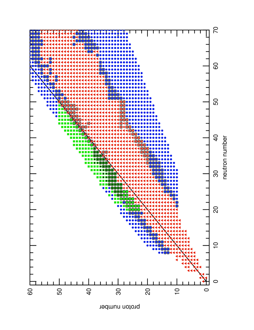
Figure 1.— Color-coded nuclear mass excesses taken from different data sources in the region of interest for the rp-process. A dark line shows the location of nuclei with $Z=N$. The actual size of the network used in these studies varied with time and model (§ 2.1). Red triangles indicate nuclei with experimentally determined mass excesses (Audi & Wapstra, 1995). Nuclei with black circles surrounding a symbol indicate that an extrapolated or interpolated mass is available from Audi & Wapstra. For those circles enclosing a red triangle, these estimated values were used. Green squares, circled or not, show where data from Brown et al. (2002) and Brown (2002) was used. These add a calculated displacement energy to the Audi-Wapstra masses for $N\geq Z$ to obtain the masses of mirror nuclei with $Z>N$. For a subset of these (black squares inside green squares) from Brown et al. (2002), the errors in the calculated displacement energies are $\sim 100\,{\mathrm{keV}}$. The solid green squares which cover a wider region are from Brown (2002) and have a larger error of several hundred keV in the calculated displacement energy due to the wider extrapolation and the possible effects of deformation in the $A=80$ mass region. In the region of $N=Z$ from $A=76-100$, the error in the mass excess is dominated by the error in the Audi & Wapstra extrapolations, which are on the order of $0.5\,{\mathrm{MeV}}$. Finally, blue circles indicate mass excess data taken from Möller et al. (1995). These were used wherever shown, (circled or uncircled).

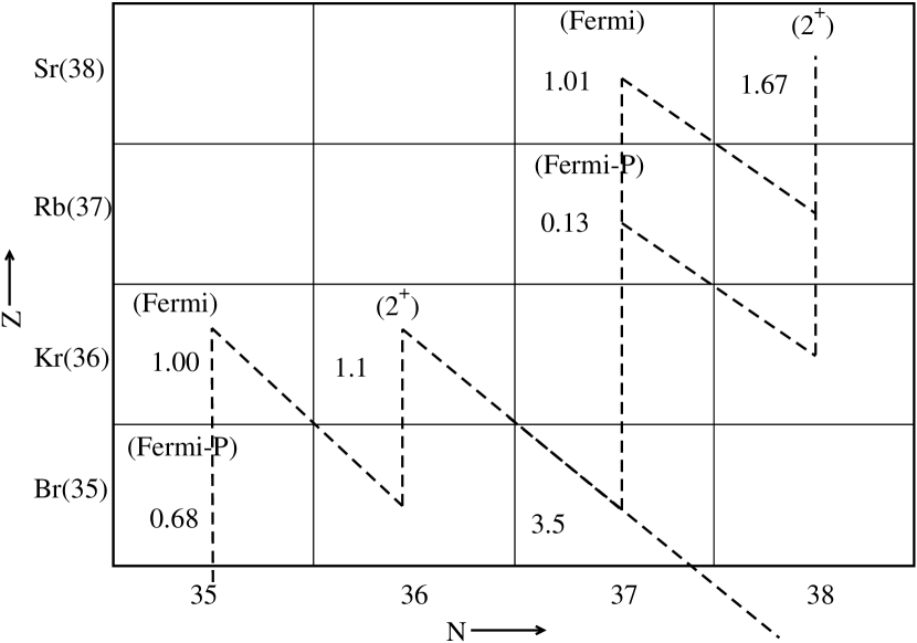
Figure 2.— Systematics of weak decays for nuclei along the rp-process path near ${{\mathrm{}}}{{\mathrm{{}^{72}}}}{\mathrm{Kr}}$. Nuclei labeled “(Fermi)” in this figure are those whose decay rates are dominated by Fermi transitions and expected to be insensitive to the temperature. Nuclei labeled “(Fermi-P)” are those whose decay rates decrease quickly with temperature. Estimates of the low-temperature decay rates for these nuclei depend largely on estimates of the nuclear partition functions. Nuclei labeled “($2^{+}$)” are those even-even nuclei whose low-temperature decay can be sensitive to the decay rate of the first excited $2^{+}$ state. The number in each box is the estimated ratio of the total ($e^{+}$ + electron capture) decay rate at $T=1.5{{\times}{10^{9}}}\,{\mathrm{K}}$, $\rho={10^{5}}\,{\mathrm{g}\,\mathrm{cm}^{-3}}$ to the ground state $e^{+}$ decay rate. The dashed black line illustrates important weak and nuclear flows during the rp-process.

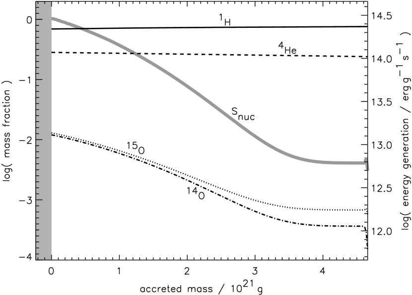
Figure 3.— Composition just prior to the first burst of Model zM (at $41,640.5\,{\mathrm{s}}$). Combined hydrogen burning by the beta-limited CNO-cycle and helium burning are responsible for a rapidly rising energy production. The total nuclear power here is $3.4{{\times}{10^{35}}}\,{\mathrm{erg}\,\mathrm{s}^{-1}}$ and the time before the burst, about one minute.

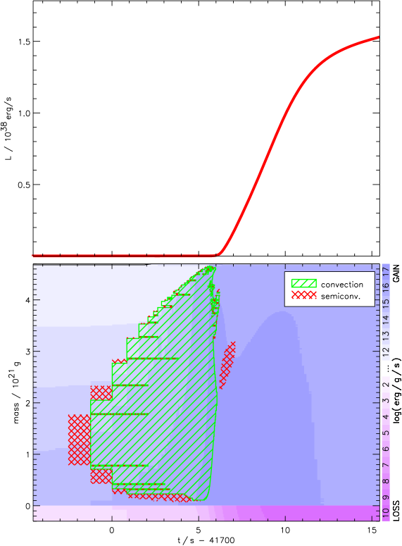
Figure 4.— The first burst in Model zM. The lower panel shows that ignition initially occurs above the composition interface, but grows over the next $6\,{\mathrm{s}}$, both outwards and inwards, to encompass the entire shell. Green hatched regions are convective; red cross hatched regions are semi-convective. The observed burst commences shortly after convection reaches the surface and has begun to recede so that the luminosity during the rise is chiefly transported by diffusion. Times are offset by $41,700\,{\mathrm{s}}$ since the beginning of accretion. Any effects due to the spreading of burning over the surface of the neutron star are ignored. Though given here for our standard choice, the rise time is sensitive to the nuclear reaction rates employed in the calculation (Fig. 20). In this and all subsequent depictions of the light curve, general relativistic effects have been ignored (§ 4.4).

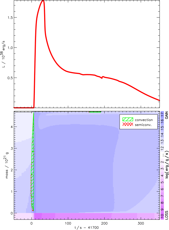
Figure 5.— The top figure shows the light curve of burst 1 of Model zM. Following the main pulse, lasting about a minute, there is a long tail, lasting perhaps $5\,\min$, powered by the continued burning of hydrogen. The shape of the light curve and its tail are sensitive to nuclear decay rates and proton capture along the rp-process path (Fig. 18). The bottom panel shows that appreciable convection only occurs prior to the rise of the pulse (see also Fig. 4). Shades of blue color indicate the nuclear energy generation rate while shades of purple indicate energy loss by neutrinos, both on a logarithmic scale. The flow of heat into the neutron star substrate is apparent.

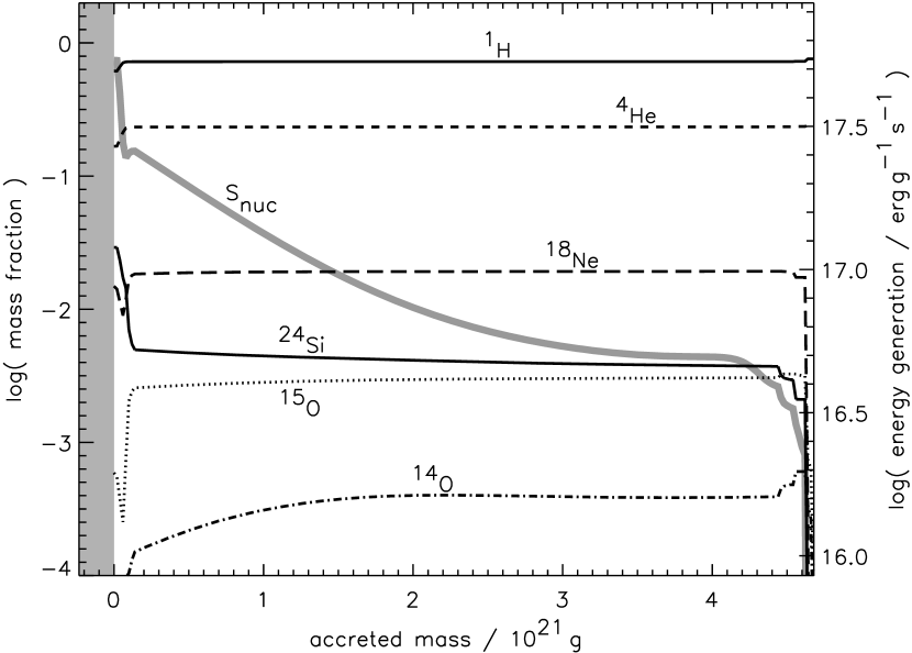
Figure 6.— Composition and nuclear energy generation during the convective phase of burst 1 in Model zM (41,705.4 s). The rp-process is responsible for producing energy and intermediate mass nuclei, the most abundant two of which are here ¹⁸Ne and ²⁴Si. Nuclei as heavy as ${{\mathrm{}}}{{\mathrm{{}^{64}}}}{\mathrm{Ge}}$ already have appreciable abundance ($2{{\times}{10^{-4}}}$ by mass). The region of near constant abundances is convective. Nuclear power is $8.3{{\times}{10^{37}}}\,{\mathrm{erg}}$ s^-1, though the luminosity transported to the surface is still only $1.3{{\times}{10^{35}}}\,{\mathrm{erg}\,\mathrm{s}^{-1}}$, invisible compared with that due to accretion. The observable burst has not started yet.

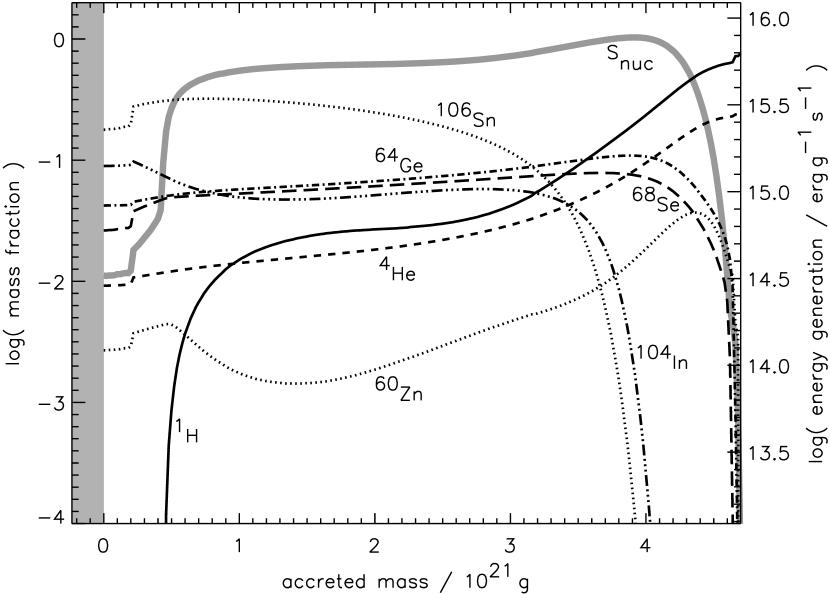
Figure 7.— Composition of Model zM and nuclear energy generation in the tail of the light curve of burst number 1 ($41,992\,{\mathrm{erg}\,\mathrm{s}^{-1}}$, Fig. 5). Though depleted at the base, considerable hydrogen remains at higher altitudes and burning continues at a high rate. The ashes at the bottom of the layer are rich in ${{\mathrm{}}}{{\mathrm{{}^{106}}}}{\mathrm{Sn}}$, the termination of the rp-process.

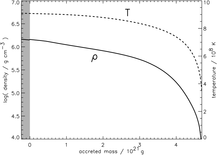
Figure 8.— Density and temperature for Model zM at the same time (41,992 s) as Fig. 7. The temperature at the base is $9.07{{\times}{10^{8}}}\,{\mathrm{K}}$ and the density, $1.44{{\times}{10^{6}}}\,{\mathrm{g}\,\mathrm{cm}^{-3}}$.

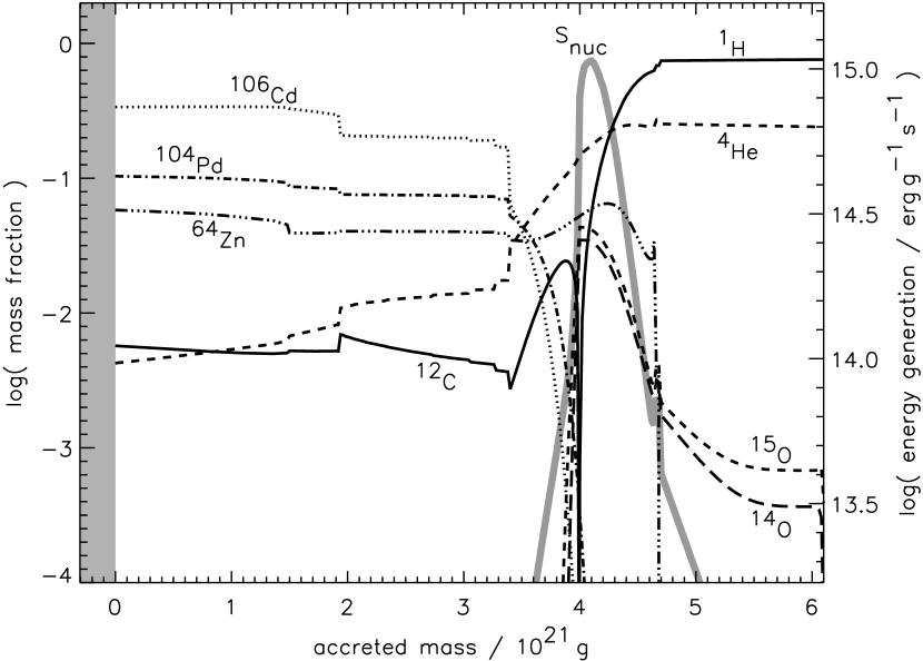
Figure 9.— Composition and energy generation at the onset of the second burst in Model zM ($5,4592\,{\mathrm{s}}$), $29\,{\mathrm{s}}$ before the flash. The ignition of the second burst occurs in the ashes of the previous one, not at the bottom of the newly accreted layer (which is located at $4.7{{\times}{10^{21}}}\,{\mathrm{g}}$). This occurrence makes the critical mass for second and subsequent bursts smaller and less sensitive to the metallicity of the accreted material. Temperature and density at the location of maximum energy generation are $9.4{{\times}{10^{5}}}\,{\mathrm{g}\,\mathrm{cm}^{-3}}$ and $2.9{{\times}{10^{8}}}\,{\mathrm{K}}$ respectively. A short time later, convection mixes the heavy ashes, e.g., ${{\mathrm{}}}{{\mathrm{{}^{64}}}}{\mathrm{Zn}}$, out into the freshly accreted layer.

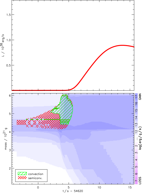
Figure 10.— Rise time and convection for burst number 2 of Model zM. This is a more typical burst for the model than the one shown in Fig. 4. Once again, convection has ceased by the time the burst first becomes visible. Following a brief convective stage lasting about 2 s, well above the bottom of the freshly accreted layer, the principal burning starts inside the ashes of the previous burst which end at $4.7{{\times}{10^{21}}}\,{\mathrm{g}}$ (Fig. 9). The intensity of the blue scale indicates nuclear burning. Note that appreciable burning occurs in the ashes of burst number 1 as the heat wave from burst number 2 propagates through. This behavior is in contrast to the neutrino losses which dominated in Fig. 4. The rise time is sensitive to the nuclear reaction rates as well as the diffusion time scale (Fig. 20).

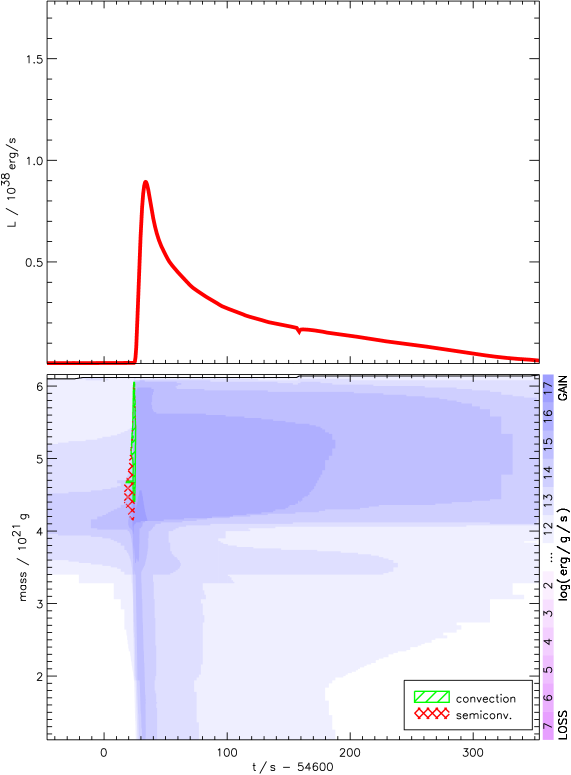
Figure 11.— Light curve for burst number 2. This briefer, less luminous second burst is more typical of all subsequent bursts in Model zM. Shades of blue indicate nuclear burning.

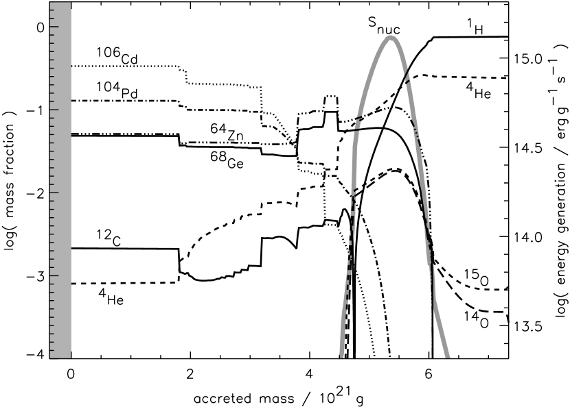
Figure 12.— Mass fractions and energy generation at the onset of the third burst in Model zM. This shows that the conditions at which the third burst ignites are very similar to those of the second. Compare with Fig. 9.

Figure 13.— Contrasting abundance distribution at the end of burst 1 and 3 in Model zM. In burst 1 the principal products were ¹⁰⁶Cd and ¹⁰⁴Pd. In burst 3 they were ${{\mathrm{}}}{{\mathrm{{}^{64}}}}{\mathrm{Zn}}$ and ${{\mathrm{}}}{{\mathrm{{}^{68}}}}{\mathrm{Ge}}$. Abundances are evaluated at the base of each accreted layer after decay.

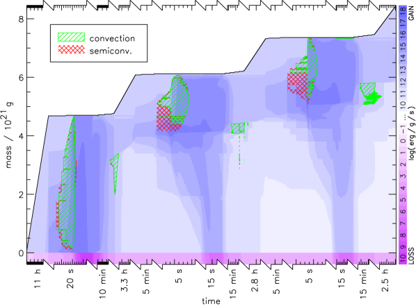
Figure 14.— Kippenhahn diagram for bursts 1, 2, and 3 in Model zM. Green hatching indicates convection; red cross hatching semi-convective regions; blue shading shows net energy generation (nuclear minus neutrino losses); and pink shading indicates net energy losses (neutrino losses exceeding nuclear energy generation). Each level of blue color indicates an increase by one order of magnitude. The $y$-axis gives the enclosed mass coordinate above the assumed neutron star substrate and the thick black line gives the total mass of accreted material. The $x$-axis gives time increasing from left to right, but different parts of the evolution are plotted on different time scale. Breaks on the axis indicate a change of time scale and and below each segment we give the length of that time interval (not the total time). The rate of change of the total mass is inversely proportional to the magnification of time in each section and is thus also and indicator of the evolutionary time scale in each section. Note repeated waves of nuclear burning in the ashes of previous bursts as heat from the current burst propagates inwards. There are also periods of convection in between bursts.

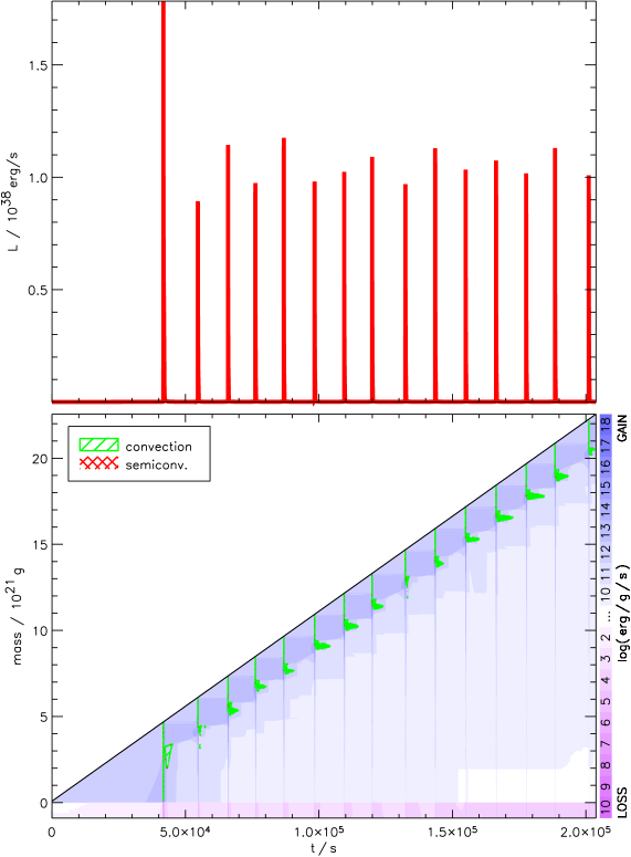
Figure 15.— Fourteen flashes from Model zM. Note the regularity of the last 13. The first is a start up transient. Note also the heat flow and burning in the ashes of earlier bursts.

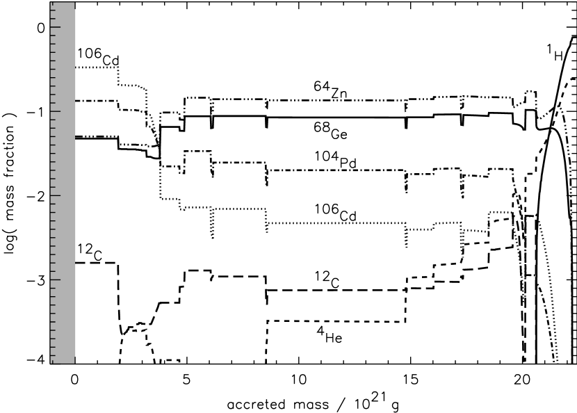
Figure 16.— Composition of the entire accreted shell after the 14^th burst in Model zM. This is the composition that will ultimately be merged into the neutron star. Aside from the anomalously heavy ashes associated with the first burst, that composition is mostly ${{\mathrm{}}}{{\mathrm{{}^{64}}}}{\mathrm{Zn}}$ and ${{\mathrm{}}}{{\mathrm{{}^{68}}}}{\mathrm{Ge}}$. Very little unburned carbon remains in these ashes.

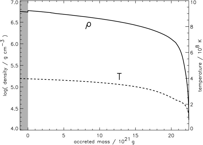
Figure 17.— Temperature and density at the end of the 14^th burst in Model zM.

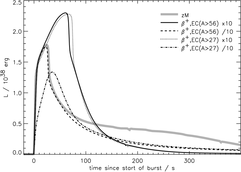
Figure 18.— Sensitivity of the light curve of the first pulse in Model zM to five choices of weak rates - standard, standard times 10 above $A=56$, standard divided by $10$ above $A=56$ and similar modifications above $A=27$. Though only the weak rates were altered, the changes reflect uncertainty in all processes, including proton capture inhibited by photodisintegration, that affect the nuclear flow. The shape of the light curve is clearly quite sensitive to the nuclear data set employed.

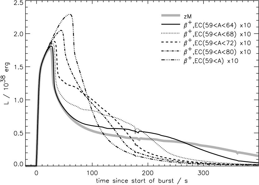
Figure 19.— Sensitivity of the light curve of the first pulse in Model zMto variations along the waiting points in the vicinity of $A=60$, $64$, and $68$. The nominal light curve is shown along with the result when all weak rates above $A=59$ are multiplied by $10$ (see Fig. 18; changing $A_{\mathrm{min}}$ from $57$ to $59$ has no effect). Also shown are the results of progressively adding in accelerations to flows in the mass ranges $A=60$–$63$, $64$–$67$, $68$–$71$, and $72$–$79$. Details of the flows for these mass ranges are given in the text. A separate calculation, not shown, in which only the decay rate of ${{\mathrm{}}}{{\mathrm{{}^{64}}}}{\mathrm{Ge}}$ was accelerated by 10 is virtually indistinguishable from the curve $e^{+}$, EC($59<A<68$) $\times 10$. Factors affecting leakage out of this single nucleus thus dominate the flow from the iron group to ${{\mathrm{}}}{{\mathrm{{}^{68}}}}{\mathrm{Se}}$. The “blip” at $180$ s is the addition of a new surface zone by accretion.

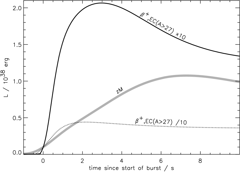
Figure 20.— Sensitivity of the rise of the light curve of the third pulse in Model zMfor three choices of weak rates - standard, standard times $10$ above $A=27$, and standard divided by $10$ above $A=28$. Flows affecting the rise time are discussed in the text. Time zero is defined as when each burst reaches ${10^{37}}\,{\mathrm{erg}\,\mathrm{s}^{-1}}$. Because this is the third burst, there have been cumulative effects from the altered rates; the critical masses of the burning layers, for example, are not the same (Tables 4 - 6), nor are the total burst energies.

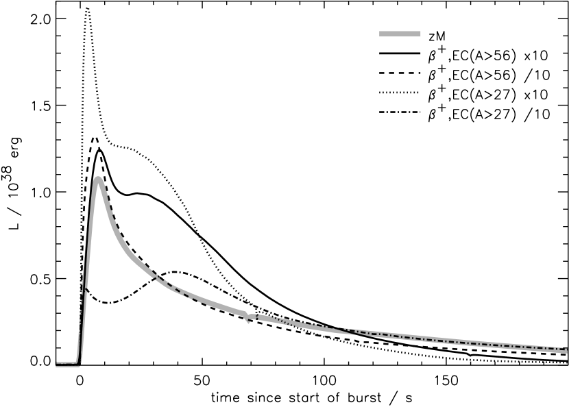
Figure 21.— Sensitivity of the light curve of the third pulse in Model zMto variation in the nuclear physics employed (see Fig. 18). This third burst may be more representative than the first one.

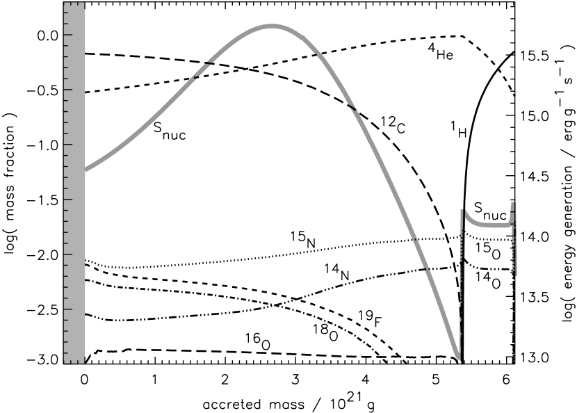
Figure 22.— Composition at the beginning of the first burst in Model Zm. Runaway here occurs in the helium burning shell where a lot of carbon ($67\,\%$ by mass) has already been synthesized. Subsequent convective mixing of the helium and hydrogen layers leads to the explosive burning of hydrogen in the presence of a large amount of carbon catalyst. The final products will not be particularly heavy.

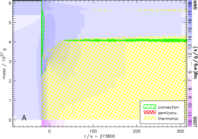
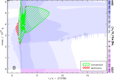
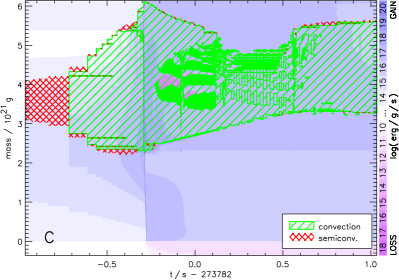
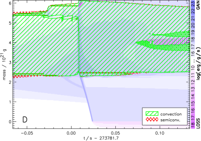
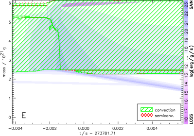
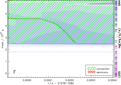
Figure 23.— Convective structure of the first burst generated in Model Zm viewed on progressively smaller time scales. Note the adjustment of the definition of zero time in each frame. A: On a time scale of minutes the burst is followed by an extended period of slow burning (indicated by blue color) and mixing by thermohaline convection (yellow cross-hatching); B: The light curve itself lasts about $13\,{\mathrm{s}}$ (similar to Fig. 26, which is for the second burst) and the burning layer is at least partly convective about half that time. The runaway and convection both begin well above the bottom of the accreted layer. The inner $2.3{{\times}{10^{21}}}\,{\mathrm{g}}$ of carbon-rich material is never convective, but does burn radiatively (note the dark blue band between $2$ and $4.5\,{\mathrm{s}}$). C: At still higher resolution, one sees the growth, both inwards and outwards, of the helium burning shell and its collision with the hydrogen layer at $-0.32\,{\mathrm{s}}$ at $5.38{{\times}{10^{21}}}\,{\mathrm{g}}$. The collision causes a mild explosion and rapid growth in the convection zone which bifurcates into hydrogen-rich and helium convective shells. D–F: Subsequent frames, at increasing resolution, show the inward propagation of the base of the hydrogen convective shell. Many thousands of stellar models were needed to follow this in this one burst. By the end, the hydrogen and helium shells are completely merged. In the radiative helium-carbon layer, at about $-0.01\,{\mathrm{s}}$ on Panel D, a weak front of ${{\mathrm{}}}{{\mathrm{{}^{22}}}}{\mathrm{Ne}}$ burning by ${{\mathrm{}}}{{\mathrm{{}^{22}}}}{\mathrm{Ne}}$($\alpha$,${{\mathrm{}}}{{\mathrm{}}}{\mathrm{n}}$) and ${{\mathrm{}}}{{\mathrm{{}^{22}}}}{\mathrm{Ne}}$($\alpha$,$\gamma$) begins to move inward. This is followed by a self-sustaining helium burning flame ignited at $+0.01\,{\mathrm{s}}$. This flame leaves behind mostly silicon and carbon, but little helium. Carbon continues to burn after the flame has passed, mostly between $-0.28\,{\mathrm{s}}$ and $-0.05\,{\mathrm{s}}$ on Panel C. The fact that convection persists (above $m\gtrsim 2.5{{\times}{10^{21}}}\,{\mathrm{g}}$), carrying high luminosity almost to the surface for over $0.1\,{\mathrm{s}}$ leads to a very rapid rise in the light curve. Unlike Model zM, where compositional “inertia” plays a big role, the critical masses, convective structures, compositions, and light curves are very similar in subsequent bursts from Model Zm.

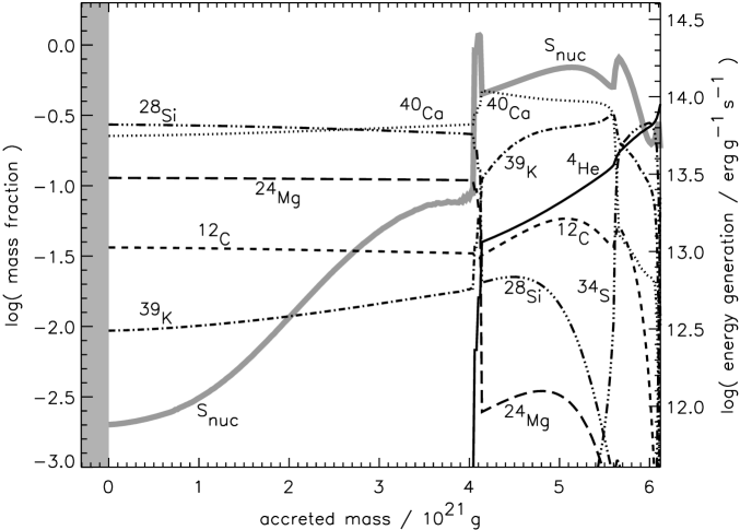
Figure 24.— Composition following the first burst in Model Zm. The time is 78 s after the beginning of the burst, well into the tail of the event whose brilliant display lasted about $30\,{\mathrm{s}}$. Some slow burning is still occurring in the helium layer. Interior to $4{{\times}{10^{21}}}\,{\mathrm{g}}$ the layer is well mixed by thermohaline convection due to a mild inverted gradient in $\bar{A}$. Only $4\,\%$ carbon remains in these inner ashes, but this will survive, since there is no helium there. Subsequent bursts leave similar ashes.

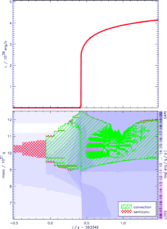
Figure 25.— Rise of the light curve for the second burst generated in Model Zm. The light curve of the first burst is similar. The rise from ${10^{37}}\,{\mathrm{erg}\,\mathrm{s}^{-1}}$ to ${{\times}{10^{38}}}\,ergs$ takes less than 1 ms (neglecting the propagation time around the neutron star). The rise from $1{{\times}{10^{38}}}\,{\mathrm{erg}\,\mathrm{s}^{-1}}$ to $2{{\times}{10^{38}}}\,{\mathrm{erg}\,\mathrm{s}^{-1}}$ takes about $100\,{\mathrm{ms}}$. Above the Eddington luminosity, $2{{\times}{10^{38}}}\,{\mathrm{erg}\,\mathrm{s}^{-1}}$, there will be radius expansion not properly followed in the present study. The excess energy will go into driving a wind.

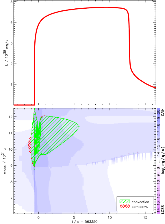
Figure 26.— Full light curve for the second burst generated in Model Zm.

Figure 27.— Repeated flashes from Model ZM. During the inter-pulse period the luminosity from accretion ($2.0{{\times}{10^{37}}}\,{\mathrm{erg}\,\mathrm{s}^{-1}}$ ) would obscure the thermal emission from the cooling ashes that is shown.

References

- Anders & Grevesse (1989) Anders, E., & Grevesse, N. 1989, Geochim. Cosmochim. Acta, 53, 197.
- Audi & Wapstra (1995) Audi, G. & Wapstra, A. H. 1995, Nucl. Phys. A, 595, 409 (AW95).
- Ayasli & Joss (1982) Ayasli, S., & Joss, P. C. 1982, ApJ, 256, 637
- Bildsten (1998) Bildsten, L. 1998, in The Many Faces of Neutron Stars, ed. R. Buccheri et al. (Dordrecht:Kluwer), 419
- Bildsten (2000) Bildsten, L. 2000, in Cosmic Explosions, the 10th Annual October Astrophysics Conference, Maryland, October 11–13, 1999, AIP Conf. 522, ed. S. Holt & W. Zhang (Woodbury NY:AIP)
- Bouchez et al. (2003) Bouchez, E., Matea, I., Korten, W., Becker, F., Blank, B., Borcea, C., Buta, A., Emsallem, A. and 16 others, 2003, Phys. Rev. Lett.90 082502-1
- Brown et al. (2002) Brown, B. A., Clement, R. R. C., Schatz, H., & Volya, A. 2002, Phys Rev C, 65, 045802
- Brown (2002) Brown, A. 2002, unpublished private communication
- Braun (1997) Braun, H., PhD thesis, Ludwig Maximilians Universität München, 1997
- Cumming (2003) Cumming, A. 2003, ApJ, in press (preprint:astroph/0306245)
- Cumming & Bildsten (2000) Cumming, A. & Bildsten, L. 2000, ApJ, 544, 453
- Cumming & Bildsten (2001) Cumming, A., & Bildsten, L. 2001, ApJ, 559, L127
- Cumming et al. (2002) Cumming, A., Morsink, S. M., Bildsten, L., Friedman, J. L., & Holz, D. E. 2002, ApJ, 564, 343
- Fisker et al. (2001) Fisker, J. L., Barnard, V., Görres, J., Langanke, K., Mártinez-Pinedo, G. & Wiescher, M. C. 2001, Atomic Data and Nuclear Data Tables, 79, 241
- Fowler (1966) Fowler, W. A. 1966, in High Energy Astrophysics, ed. L. Gratton, (New York: Academic Press), p 313
- Fuller et al. (1982) Fuller, G. M., Fowler, W. A. & Newman, M. J. 1982, ApJ252, 715 (FFN)
- Fuller et al. (1985) Fuller G. M., Fowler, W. A. and Newman, M. J. 1985, ApJ, 293, 1
- Fujimoto et al. (1981) Fujimoto, M. Y., Hanawa, T., & Miyaji, S. 1981, ApJ, 247, 267
- Fujimoto et al. (1987) Fujimoto, M. Y., Sztajno, M., Lewin, W. H. G., & van Paradijs, J. 1987, ApJ, 319, 902
- Fushiki & Lamb (1987) Fushiki, I., & Lamb, D. Q. 1987,ApJ,323, L55
- Fushiki et al. (1992) Fushiki, I., Taam, R. E., Woosley, S. E., & Lamb, D. Q. 1992, ApJ, 390, 634
- Galloway et al. (2003) Galloway, D. K., Cumming, A., Kuulkers, E., Bildsten, L., Chakrabarty, D., & Rothschild, R. E. 2003, ApJ, submitted
- Hanawa & Fujimoto (1984) Hanawa, T.; Fujimoto, M. Y.1984, PASJ, 36, 199
- Hansen & van Horn (1975) Hansen, C. J., & van Horn, H. M. 1975, ApJ, 195, 735
- Joss (1977) Joss, P. C. 1977, Nature, 270, 310
- Kippenhahn et al. (1980) Kippenhahn, R., Ruschenplatt, G., & Thomas, H.-C. 1980, A&A, 91, 175
- Koike et al. (1999) Koike, O., Hashimoto, M., Arai, K., & Wanajo, S. 1999, A&A, 342, 464
- Kuulkers et al. (2002) Kuulkers, E., in’t Zand, J. J. M., van Kerkwijk, M. H., Cornelisse, R., Smith, D. A., Heise, J., Bazzano, A., Cocchi, M., Natalucci, L., & Ubertini, P. 2002, A&A, 382, 503
- Langanke & Martinez-Pinedo (2000) Langanke, K. & Martinez-Pinedo, G. 2001, Nucl. Phys. A, 673, 481 (LMP)
- Lewin et al. (1993) Lewin, W. H. G., van Paradijs, J., & Taam, R. E. 1993, Space Science Rev., 62, 223
- Lewin et al. (1995) Lewin, W. H. G., van Paradijs, J., & Taam, R. E. 1995, in X-Ray Binaries, ed. Lewin et al., (Cambridge Univ. Press), 175
- Möller et al. (1995) Möller, P., Nix, J. R., Myers, W.D. & Swiatecki, W. J. 1995, Atomic Data and Nuclear Data Tables, 59, 185
- Möller et al. (1997) Möller, P., Nix, J. R., Kratz, K.-L. 1997, Atomic Data and Nuclear Data Tables, 66, 131
- Narayan & Heyl (2003) Narayan, R., & Heyl, J. S. 2003, ApJ, submitted (astro-ph/0303447)
- Ormand (1997) Ormand, W. E. 1997, Phys. Rev. C, 55, 2407
- Pruet & Fuller (2002) Pruet, J. & Fuller, G. M. 2002, ApJS, in press
- Rauscher & Thielemann (2000) Rauscher, T. & Thielemann, F.-K. 2000, Atomic Data and Nuclear Data Tables, 75, 1
- Rauscher et al. (2000) Rauscher, T., Rembges, F., Schatz, H., Wiescher, M., Thielemann, F.-K. 2000,in ”The Beta-Decay, from Weak Interaction to Nuclear Structure”, eds. P. Dessagne, A. Michalon, C. Mieh (IRes, Strasbourg), p. 51.
- Rembges (1999) Rembges, J.-F. 1999, PhD thesis, Universität Basel
- Schatz et al. (1998) Schatz, H., Aprahamian, A., Goerres, J., Wiescher, M., Rauscher, T., Rembges, J. F., Thielemann, F.-K., Pfeiffer, B., Moeller, P., Kratz, K.-L., Herndl, H., Brown, B. A. & Rebel, H. 1998, Phys. Rep., 294, 167
- Schatz et al. (2001a) Schatz, H., Aprahamian, A., Barnard, V., Bildsten, L., Cumming, A., Ouellette, M., Rauscher, T., Thielemann, F.-K., & Wiescher, M. 2001, Phys. Rev. Lett., 86, 3471
- Schatz et al. (2001b) Schatz, H., Aprahamian, A., Barnard, V., Bildsten, L., Cumming, A., Ouellette, M., Rauscher, T., Thielemann, F.-K., & Wiescher, M. 2001, Nuc Phys A, 688, 150c
- Cumming et al. (2003) Schatz, H., Bildsten, L., & Cumming, A. 2003a, ApJ, 583, L87
- Schatz et al. (2003) Schatz, H., Bildsten, L., Cumming, A., & Ouellette, M. 2003, in 7th International Symposium on Nuclei in the Cosmos (NIC7), ed. S. Kubono, T. Teranishi, T. Kajino, K. Nomoto and I. Tanihata, Nucl. Phys. A, 718, 247
- Spitkovsky et al. (2002) Spitkovsky, A., Levin, Y., & Ushomirsky, G. 2002, ApJ, 566, 1018
- Strohmayer & Bildsten (2003) Strohmayer, T., & Bildsten, L. 2003, in Compact Stellar X-Ray Sources, eds. W. H. G. Lewin & M. van der Klis (Cambridge: Cambridge University Press)
- Strohmayer & Brown (2002) Strohmayer, T., & Brown, E. F. 2002, ApJ, 566, 1045
- Taam (1980) Taam, R. E. 1980, ApJ, 241, 358
- Taam et al. (1993) Taam, R. E., Woosley, S. E., Weaver, T. A., & Lamb, D. Q. 1993, ApJ, 413, 324
- Taam et al. (1996) Taam, R. E., Woosley, S. E., & Lamb, D. Q. 1996, ApJ, 459, 271
- Thielemann et al. (2001) Thielemann, F.-K., Brachwitz, F., Freiburghaus, C., Kolbe, E., Martinez-Pinedo, G., Rauscher, T., Rembges, F.; Hix, W. R., and nine others 2001, Prog. Part. Nucl. Phys. 46, 5.
- van Paradijs et al. (1988) van Paradijs, J., Penninx, W., & Lewin, W. H. G. 1988, MNRAS, 233, 437
- Wallace & Woosley (1981) Wallace, R. K., & Woosley, S. E. 1981, ApJ, 45, 389
- Wallace & Woosley (1984) Wallace, R. K., & Woosley, S. E. 1984, in High Energy Transients in Astrophysics, ed. S. Woosley, AIP Conf Proc. No. 115, p. 319.
- Weaver et al. (1978) Weaver, T. A., Zimmerman, G. B., & Woosley, S. E. 1978, ApJ, 225, 1021
- Woosley & Taam (1976) Woosley, S. E., & Taam, R. E. 1976, Nature, 263, 101
- Woosley & Weaver (1984) Woosley, S. E., & Weaver, T. A. 1984, AIP Conf. Proc. No. 115, High Energy Transients in Astrophysics, ed. S. Woosley, p. 273
- Woosley et al. (2002) Woosley, S. E., Heger, A., & Weaver, T. A. 2002, RMP, 74, 1015
- Zingale et al. (2003) Zingale, M. et al. 2003, in 3D Stellar Evolution, ASP Conf. Proc. 293, ed. Sylvain Turcotte, Stefan C. Keller, & Robert M. Cavallo., p.329