On characterising the variability properties of X-ray light curves from active galaxies

Abstract

We review some practical aspects of measuring the amplitude of variability in ‘red noise’ light curves typical of those from Active Galactic Nuclei (AGN). The quantities commonly used to estimate the variability amplitude in AGN light curves, such as the fractional rms variability amplitude, $F_{\rm{var}}$, and excess variance, $\sigma_{\rm{XS}}^{2}$, are examined. Their statistical properties, relationship to the power spectrum, and uses for investigating the nature of the variability processes are discussed. We demonstrate that $\sigma_{\rm{XS}}^{2}$ (or similarly $F_{\rm{var}}$) shows large changes from one part of the light curve to the next, even when the variability is produced by a stationary process. This limits the usefulness of these estimators for quantifying differences in variability amplitude between different sources or from epoch to epoch in one source. Some examples of the expected scatter in the variance are tabulated for various typical power spectral shapes, based on Monte Carlo simulations. The excess variance can be useful for comparing the variability amplitudes of light curves in different energy bands from the same observation. Monte Carlo simulations are used to derive a description of the uncertainty in the amplitude expected between different energy bands (due to measurement errors). Finally, these estimators are used to demonstrate some variability properties of the bright Seyfert 1 galaxy Markarian 766. The source is found to show a strong, linear correlation between rms amplitude and flux, and to show significant spectral variability.

1 Introduction

One of the defining characteristics of Active Galactic Nuclei (AGN) is that their X-ray emission is variable. X-ray light curves from Seyfert 1 galaxies show unpredictable and seemingly aperiodic variability (Lawrence et al. 1987; M^cHardy 1989). Such random variability is often referred to as noise, meaning that it is the result of a stochastic, as opposed to deterministic, process. In this context the ‘noise’ is intrinsic to the source and not a result of measurement errors (such as Poisson noise), i.e. the signal itself is the output of a noise process.

One of the most common tools for examining AGN variability (and noise processes in general) is the fluctuation Power Spectral Density (PSD) which represents the amount of variability power (mean of the squared amplitude) as a function of temporal frequency (timescale^-1). The high frequency PSDs of Seyferts are usually well-represented by power-laws over a broad range of frequencies ($\mathcal{P}(f)\propto f^{-\alpha}$, where $\mathcal{P}(f)$ is the power at frequency $f$) with slopes $\alpha=1-2$ (Green, M^cHardy & Lehto, 1993; Lawrence & Papadakis, 1993; Edelson & Nandra, 1999; Uttley, M^cHardy & Papadakis, 2002; Vaughan, Fabian & Nandra 2003; Markowitz et al. 2003). Such a spectrum, with a slope $\alpha\mathrel{\hbox{\hbox to0.0pt{\hbox{\lower 4.0pt\hbox{$\sim$}}\hss}\hbox{$>$}}}1$ is usually called ‘red noise’ (for an introduction to red noise see Press 1978).

If Seyfert 1 light curves are viewed as the product of a stochastic (in this case red noise) process then the specific details of each individual light curve provide little physical insight. Each light curve is only one realisation of the underlying stochastic process, i.e. it is one of the ensemble of random light curves that might be generated by the process. Each new realisation will look different and these changes are simply statistical fluctuations inherent in any stochastic process (as opposed to changes in the nature of the process itself). Therefore one should expect two light curves to have different characteristics (such as mean and variance) even if they are realisations of the same process. On the other hand, data from deterministic processes, for example the energy spectrum of a non-varying source or the light curve of a strictly periodic source (such as a pulsar), should be repeatable within the limits set by the measurement errors.

It is the average properties of the variability (such as the PSD) that often provide most insight into the driving process. For example, the PSD of any real red noise process cannot continue as a steep power-law indefinitely to longer timescales or the integrated variability power would diverge. Therefore the PSDs of AGN variability must break to a flatter index at low frequencies; the position of such a break would represent a characteristic variability timescale and may yield information about the underlying driving process. Recent timing studies have indeed found evidence that the steep power-law PSDs of Seyfert 1s show a flattening, or turnover, at low frequencies (Edelson & Nandra 1999; Uttley et al. 2002; Markowitz et al. 2003).

In many cases however the data are not adequate for PSD analysis. In these situations the variability is usually described in terms of the statistical moments (e.g. the sample mean and variance, etc.). However, due to the stochastic nature of red noise variability there is a large degree of randomness associated with these quantities. In practice this means that it is difficult to assign meaningful errors to the variance. This in turn makes it difficult to quantitatively compare variances, say from repeated observations of the same source (and thereby test whether the variability is stationary). Such an analysis might be desirable; it could in principle reveal changes in the ‘state’ of the source if its variability properties were found to evolve with time. This paper discusses this and related problems that are encountered when examining the variability properties of AGN. Particular emphasis is placed on the mathematical properties and implications of the inherent randomness in the variability. The mathematical details are well understood from the general theory of stochastic processes (e.g. Priestley 1981 for spectral analysis) but some of the practical consequences for AGN observations have not been discussed in detail. On the basis of simulated data some recipes are developed that may serve as a useful guide for observers wishing make quantitative use of their variability analysis without the recourse to e.g. extensive Monte Carlo simulations.

The paper is organised as follows. Section 2 defines the estimators to be discussed (namely the periodogram and the variance). Simulated data are used to illustrate various aspects of these estimators; section 3 describes methods for producing artificial red noise time series. Section 4 discusses the stationarity of time series. Sections 5 and 6 discuss two sources of uncertainty associated with measuring variability amplitudes, the first due to the stochastic nature of the variability and the second due to flux measurement errors. Section 7 gives an example using a real XMM-Newton observation of Mrk 766. Finally, a brief discussion of these results is given in section 8 and the conclusions are summarised in section 9.

2 Estimating the Power Spectral Density

The PSD defines the amount of variability ‘power’ as a function of temporal frequency. It is estimated by calculating the periodogram (Priestley 1981; Bloomfield 2000).

For an evenly sampled light curve (with a sampling period $\Delta T$) the periodogram is the modulus-squared of the Discrete Fourier Transform (DFT) of the data (Press et al. 1996). For a light curve comprising a series of fluxes $x_{i}$ measured at discrete times $t_{i}~{}(i=1,2,\ldots,N)$:

$$|DFT(f_{j})|^{2}=\left|\sum_{i=1}^{N}x_{i}~{}\mathrm{e}^{2\mathrm{\pi}\mathrm{i}f_{j}t_{i}}\right|^{2}=$$

$$\qquad\left\{\sum_{i=1}^{N}x_{i}~{}\cos(2\mathrm{\pi}f_{j}t_{i})\right\}^{2}+\left\{\sum_{i=1}^{N}x_{i}~{}\sin(2\mathrm{\pi}f_{j}t_{i})\right\}^{2},$$ (1)

at $N/2$ evenly spaced frequencies $f_{j}=j/N\Delta T$ (where $j=1,2,\ldots,N/2$), $f_{N/2}=1/2\Delta T$ is the Nyquist frequency, $f_{\rm Nyq}$. Note that it is customary to subtract the mean flux from the light curve before calculating the DFT. This eliminates the zero-frequency power. The periodogram, $P(f_{j})$, is then calculated by choosing an appropriate normalisation $A$ (see Appendix A for more on periodogram normalisations). For example

$$P(f_{j})=A|DFT(f_{j})|^{2}=\frac{2\Delta T}{N}|DFT(f_{j})|^{2}.$$ (2)

If the time series is a photon counting signal such as normally encountered in X-ray astronomy, and is binned into intervals of $\Delta T$, the effect of Poisson noise is to add an approximately constant amount of power to the periodogram at all frequencies. With the above normalisation this constant Poisson noise level is $2\bar{x}$ (assuming the light curve is not background subtracted).

2.1 Statistical properties of the periodogram

The periodogram of a noise process, if measured from a single time series, shows a great deal of scatter around the underlying PSD. In particular, the periodogram at a given frequency [$P(f)$] is scattered around the PSD [$\mathcal{P}(f)$] following a $\chi^{2}$ distribution with two degrees of freedom (van der Klis 1989):

$$P(f)=\mathcal{P}(f)\chi_{2}^{2}/2,$$ (3)

where $\chi_{2}^{2}$ is a random variable distributed as $\chi^{2}$ with two degrees of freedom, i.e. an exponential distribution with a mean and variance of two and four, respectively. The periodogram is distributed in this way because the real and imaginary parts of the DFT are normally distributed for a stochastic process (section 6.2 of Priestley, 1981; Jenkins & Watts 1968). The expectation value of the periodogram is equal to the PSD but its standard deviation is 100 per cent, leading to the larger scatter in the periodogram (see Fig. 1). See Leahy et al. (1983), van der Klis (1989), Papadakis & Lawrence (1993), Timmer & König (1995) and Stella et al. (1997) for further discussion of this point.

When applied to real data the periodogram is an inconsistent estimator of the PSD, meaning that the scatter in the periodogram does not decrease as the number of data points in the light curve increases (Jenkins & Watts 1968). In order to reduce this scatter the periodogram must be smoothed (averaged) in some fashion. As the number of data points per bin increases (either by binning over frequencies or averaging over many data segments) the scatter in the binned periodogram decreases, i.e. the averaged periodogram is a consistent estimator of the PSD (see Papadakis & Lawrence 1993 and van der Klis 1997 for more on binned periodogram estimates). A further point is that periodograms measured from finite data tend to be biased by windowing effects which further complicate their interpretation (van der Klis 1989; Papadakis & Lawrence 1993; Uttley et al. 2002 and see below).

2.2 Integrated power

The integral of the PSD between two frequencies ($f_{1}$ and $f_{2}$) yields the contribution to the expectation value of the (‘true’) variance due to variations between the corresponding timescales ($1/f_{1}$ and $1/f_{2}$). This result follows from Parseval’s theorem (see e.g. van der Klis 1989)

$$\langle S^{2}\rangle=\int_{f_{1}}^{f_{2}}\mathcal{P}(f)df.$$ (4)

Correspondingly, for a discrete time series the integrated periodogram yields the observed variance for that particular realisation

$$S^{2}=\sum_{j=1}^{N/2}P(f_{j})\Delta f,$$ (5)

where $\Delta f$ is the frequency resolution of the DFT ($\Delta f=1/N\Delta T$). The total variance of a real light curve is equal to its periodogram integrated over the frequency range $f_{1}=1/N\Delta T$ to $f_{\rm Nyq}=1/2\Delta T$.

The sample variance (which will differ from observation to observation) is given by:

$$S^{2}=\frac{1}{N-1}\sum_{i=1}^{N}(x_{i}-\bar{x})^{2},$$ (6)

where $\bar{x}$ is the arithmetic mean of $x_{i}$. In the limit of large $N$ these two variance estimates are identical. The normalised variance is simply $S^{2}/\bar{x}^{2}$.

Figure 1: Simulated time series (left) and their periodograms (right). The upper panel shows a ‘flicker noise’ time series which has a $f^{-1}$ PSD. The lower panel shows a ‘random walk’ time series with a $f^{-2}$ PSD. Note the large scatter in the periodogram (dots) around the underlying PSD (solid line). It is clear that the time series with the steeper PSD shows more power in long-term variability while the time series with the flatter PSD shows relatively more power in short term variability (flickering). The two series were generated using the same random number sequence.

3 Simulating red noise light curves

3.1 Algorithms

In order to elucidate the properties of the variance of red noise data, random light curves were generated from power-law PSDs similar to those of AGN. Fig. 1 shows two artificial time series and their periodograms. It is worth reiterating that the large scatter in the periodograms is an intrinsic property of stochastic processes – it does not depend on the number of data points and is not related to Poisson noise in the data.

These artificial time series were produced using the algorithm of Timmer & König (1995). This generates random time series with arbitrary broad-band PSD, correctly accounting for the intrinsic scatter in the powers (i.e. equation 3). Other methods of generating random light curves include the related ‘summing of sines’ method (Done et al. 1992). Note that it is not correct to randomise only the phases of the component sine functions, their amplitudes must also be randomised. Otherwise this method does not account for this intrinsic scatter in the powers. Shot-noise models can produce red noise time series with certain PSD shapes (see Lehto 1989). There also exist various mathematical tricks for producing data with specific power-law PSD slopes. Data with a $\alpha=1$ PSD (often called ‘flicker noise’) can be generated using the half-integral method outlined in Press (1978), while $\alpha=2$ (‘random walk’) data can be generated using a first-order autoregressive process (AR[1]), essentially a running sum of Gaussian deviates (see Deeming 1970 and Scargle 1981 for more on such methods). The method of Timmer & König (1995) is used below as this can generate time series from an arbitrary PSD and is computationally efficient.

3.2 Simulating ‘realistic’ data

Some caution should be applied when using these routines to produce artificial time series. As mentioned briefly in the previous section, periodograms measured from real data tend to be biased by windowing effects. For uninterrupted but finite observations data of red noise processes the most important of these effects is ‘red noise leak’ – the transfer of power from low to high frequencies by the lobes of the window function (see e.g. Deeter & Boynton 1982; van der Klis 1997). If there is significant power at frequencies below the lowest frequency probed by the periodogram (i.e. on timescales longer than the length of the observation) this can give rise to slow rising or falling trends across the light curve. These trends contribute to the variance of the light curve. Thus variability power ‘leaks’ into the data from frequencies below the observed frequency band-pass. The degree to which this occurs, and the resultant bias on the measured periodogram, depend on the shape of the underlying PSD and the length of the observation (Papadakis & Lawrence 1995; Uttley et al. 2002). For flat PSD slopes ($\alpha<1.5$) the amount of leakage from low frequencies is usually negligible.

Since AGN light curves usually contain significant power on timescales longer than those probed (see section 4.1) the effects of red noise leak must be included in simulations of AGN light curves. This can be achieved by using the Timmer & König (1995) algorithm to generate a long light curve from a PSD that extends to very low frequencies and then using a light curve segment of the required length. Data simulated in such a fashion will include power on timescales much longer than covered in the short segment. The effects of measurement errors (e.g. Poisson noise) can be included in the simulations using standard techniques (e.g. Press et al. 1996).

4 Stationarity

A stationary process is one for which the statistical properties (such as mean, variance, etc.) do not depend on time. Fig. 2 shows an artificial red noise time series together with its mean and variance measured every 20 data points. The simulation was produced from a single, well-defined PSD (which did not vary). The process is therefore stationary. It would have been reasonable to expect the resulting time series (a realisation of the process) to appear stationary. This is not the case however; both the mean and variance change with time (panels 2 and 3). This has nothing whatsoever to do with measurement errors - the simulation has zero errors. This simulation demonstrates that, when dealing with red noise, fluctuations in variance are not sufficient to claim the variability process is non-stationary.

As the purpose of time series analysis is to gain insight into the process, not the details of any specific realisation, a more robust approach is needed to determine whether these data were produced by a time-stationary process or a non-stationary process. It would be more insightful to consider whether the expectation values of the characteristics (such as the variance) are time-variable. The expectation values should be representative of the properties of the underlying process, not just any one realisation. See section 1.3 of Bendat & Piersol (1986) for a discussion of this point.

Figure 2: Panel 1: Simulated red noise time series (with a $f^{-2}$ PSD) with $N=2800$ points. Panel 2 and 3: mean and variance measured from segments of 20 points (calculated using equation 6). The variances follow a distribution of the form shown in the bottom panel of Fig. 3. (Note the variance is plotted on a logarithmic scale.) Panel 4: averaged variance measured by binning the individual variances into groups of 20 consecutive estimates. The errors are the standard error on the mean (equation 4.14 of Bevington & Robinson 1992). These averaged variances are consistent with staying constant. In other words, although the instantaneous value of the variance fluctuates, its expectation value is consistent with constant (i.e. a stationary process). Panel 5: fractional rms amplitude ($\sqrt{S^{2}/\bar{x}^{2}}$) measured from segments of 20 points. Panel 6: averaged fractional rms amplitude measured by binning the individual amplitudes into groups of 20. The fractional amplitude is anti-correlated with the light curve because $\langle S^{2}\rangle$ is constant but $F_{\rm var}$ is normalised by the light curve flux.

4.1 Weak non-stationarity

For a process with a steep red noise PSD ($\alpha\geq 1$), the integrated periodogram will diverge as $f\rightarrow 0$. This means that (following equation 4) the variance of a red noise time series with a steep PSD will diverge with time. In this case there is no well-defined mean; Press & Rybicki (1997) describe this form of variability as ‘weakly non-stationary.’ For time series with power spectra flatter than this the variance converges as $f\rightarrow 0$, thus for a white noise process with a flat PSD ($\alpha=0$), the variance will converge as the observation length increases, and there will be a well-defined mean on long timescales.

Of course, for any real process the PSD must eventually flatten such that the power does not diverge (i.e. $\alpha<1$ on sufficiently long timescales). Thus, weak non-stationarity is entirely due to observations sampling only the steep part of the PSD of a source. But in AGN this flattening occurs on timescales much longer than those probed by typical observations. For instance, XMM-Newton observations of AGN typically last for $\sim{\rm few}\times 10^{4}$ s whereas in many objects the PSD is steep until $>10^{5}$ s and in some cases probably much longer (Edelson & Nandra 1999; Uttley et al. 2002; Markowitz et al. 2003). Therefore on the timescales relevant for most X-ray observations, AGN light curves should be considered weakly non-stationary.

4.2 Stochasticity

Figure 3: Distribution of variances in time series with three different PSD shapes: $f^{0}$ (top), $f^{-1}$ (middle) and $f^{-2}$ (bottom). Each distribution is derived from 50,000 realisations. As the PSD gets steeper the distribution of variances becomes less Gaussian and more like a $\chi^{2}$ distribution with a low effective degrees of freedom.

Fluctuations in the statistical moments (such as mean and variance) of a light curve are intrinsic to red noise processes. Therefore, even in the absence of measurement errors (e.g. no Poisson noise) the means and variances of two light curves produced by exactly the same process can be significantly different. This can be seen in Fig. 2 (panels 2 and 3), where each 20 point segment of the light curve shows a different mean and variance. These random fluctuations in variance are however governed by the normal statistical rules of noise processes and can thus be understood in a statistical sense.

Any given series is only one realisation of the processes and its periodogram will show the scatter predicted by equation 3. The integrated periodogram (which gives the variance; equation 5) will therefore be randomly scattered around the true value for the PSD of the process. The variance in a specific time series is given by

$$S^{2}=\frac{1}{N\Delta T}\sum_{i=1}^{N/2}\mathcal{P}(f_{i})\chi_{2}^{2}/2,$$ (7)

i.e. the variance of a given realisation is a sum of $\chi_{2}^{2}$ distributions weighted by the PSD. (This assumes biases such as red noise leak are not significant. If this is not true then these biases will further distort the distribution of variances.) It is the expectation value of the variance that is representative of the integrated power in the PSD, and thus the average amplitude of the variability process (eqn. 4). Thus, while the expectation value of the variance is equal to the integrated PSD, each realisation (time series) of the same process will show a different variance even if the parent variability process is stationary. This is particularly important for steep PSD time series (i.e. weakly non-stationary data) since the variance does not converge as more data are collected. Only if the time series spans timescales on which the integrated power converges at low frequencies (i.e. $\alpha<1$) will the variance converge as the length of time series increases.

These points are illustrated by Fig. 3, which shows the distributions of variances in random time series with three different PSD slopes ($\alpha=0,1,2$). This plot was produced by generating 50,000 random time series (each 100 points long) for each PSD slope and measuring the variance of each one. The scatter in the variance is entirely due to random fluctuations between different realisations because the PSD normalisation was kept fixed and no instrumental noise was added. The shape of the distribution of variances can be seen to depend on the PSD slope.

Consider a white noise process ($\alpha=0$, i.e. $\mathcal{P}(f)=const$). The periodogram of each realisation is randomly scattered around its flat PSD. Following equation 7 the variance is simply the sum of the $N/2$ $\chi_{2}^{2}$-distributed powers in the periodogram, and these are evenly weighted (PSD is constant). The sum of $N/2$ $\chi_{2}^{2}$ distributions follows a $\chi_{N}^{2}$ distribution. This tends to a normal distribution as $N$ increases. Thus the variance of a white noise process is approximately normally distributed (as can be seen in Fig. 3) and converges as $N$ increases. The fractional standard deviation of $\chi_{N}^{2}$ is given by $\sqrt{2/N}$, so for the 100 point light curves used the (1$\sigma$) fractional width of the variance distribution is $\approx 14.1$ per cent, in agreement with the simulations (Fig. 3, top panel).

For time series with steeper PSDs the lower frequency periodogram points contribute more strongly to the sum than the higher frequency points. The variance of such a time series is therefore dominated by a few low frequency powers and thus resembles a $\chi_{\nu}^{2}$ distribution with low ‘effective degrees of freedom.’ The distribution of variances in red noise data is dependent on the underlying PSD and is, in general, non-Gaussian (Fig. 3). The fractional standard deviation of $\chi_{\nu}^{2}$ is $\sqrt{2/\nu}$, which tends to unity as the PSD gets steeper (i.e. as effective $\nu\rightarrow 2$). Thus the largest fluctuations in variance (up to a limit of $\sim 100$ per cent rms) are expected to result from very steep PSD slopes.

5 Intrinsic scatter in variance

As discussed above, when examining AGN light curves one should expect random changes in the mean and variance with time (between segments of a long observation or between observations taken at different epochs). This is true even if the measurement errors are zero and does not depend on the number of data points used (due to the weak non-stationarity). However, it is also possible that the underlying process responsible for the variability itself changes with time (e.g. the PSD changes), in which case the variability is non-stationary in a more meaningful sense – ‘strongly non-stationary.’ Such changes in the variability process could provide insight into the changing physical conditions in the nuclear regions. On the other hand the random changes expected for a red noise process yield no such physical insight. The question thus arises: how does one tell, from a set of time series of the same source, whether they were produced by a strongly non-stationary process? In other words, is it possible to differentiate between differences in variance caused by real changes in the variability process (physical changes in the system), and random fluctuations expected from red noise (random nature of the process)?

If the process responsible for the variability observed in a given source is stationary then its PSD is constant in time. The expectation value of the absolute (un-normalised) variance will therefore be the same from epoch to epoch, but the individual variance estimates will fluctuate as discussed in section 4.2. This makes it difficult to judge, from just the variances of two light curves taken at two epochs, whether they were produced by a stationary process. Given sufficient data it is, however, possible to test whether the expectation values of the variance (estimated from an ensemble of light curves) at two epochs are consistent with a stationary process.

5.1 Comparing PSDs

The methods most frequently employed involve comparing the PSDs (estimated from the binned periodogram) at different epochs. If the PSDs show significant differences (at a given confidence level) the variability process can be said to be strongly non-stationary. As an example of this, the PSDs of X-ray binaries evolve with time, and the way in which the variability properties evolve provides a great deal of information on the detailed workings of these systems (see e.g. Belloni & Hasinger 1990; Uttley & M^cHardy 2001; Belloni, Psaltis & van der Klis 2002; Pottschmidt et al. 2002).

Papadakis & Lawrence (1995) suggested a method suitable for testing whether large AGN datasets display evidence for strongly non-stationary variability. Again this method works by comparing the PSDs from different time intervals, in this case by determining whether the differences between two periodograms are consistent with the scatter expected based on equation 3. In particular, they define a statistic $s$ based on the ratio of two normalised periodograms. If $s$ deviates significantly from its expected value for stationary data (if $\langle s\rangle=0$) then the hypothesis that the data are stationary can be rejected (at some confidence level).

5.2 Comparing variances

A different approach is compare variances $S_{i}$ derived from $M$ observations of the same source (either segments of one long observation or separate short observations). In order to test whether the $S_{i}$ differ significantly (i.e. more than expected for a red noise process) a measure of the expected scatter is required. This error could be obtained directly from the data (by measuring the standard deviation of multiple estimates) or through simulations (based on an assumed PSD shape).

5.2.1 Empirical error on variance

An empirical estimate of the mean and standard deviation of the variance can be made given $M$ non-overlapping data segments. The $M$ segments each yield an estimate of the variance, $S_{i}$. Each of these is an independent variable of (in general) unknown but identical distribution (unless the process is strongly non-stationary). The central limit theorem dictates that the sum of these will become normally distributed as $M$ increases. Therefore by averaging the $M$ variance estimates it is possible to produce an averaged variance ($\langle S^{2}\rangle$) and assign an error bar in the usual fashion (e.g. equation 4.14 of Bevington & Robinson 1992). This gives a robust estimate of the variance and the standard deviation of the $M$ variances around the mean gives an estimate of the uncertainty on the mean variance.

If several sets of data segments are acquired it is therefore possible to compare the mean variance of each set statistically (since each has an associated uncertainty). For example, with two long XMM-Newton observations of the same source, taken a year apart, one could measure the variance for each observation (by breaking each into short segments and taking the mean variance of the segments). Thus it would be possible to test whether the variability was stationary between the two observations. This method of estimating the mean and standard deviation of the variance requires a large amount of data. Of order $N\times M=20\times 20=400$ data points are needed to produce a single well-determined estimate of the mean variance and its error. A typical XMM-Newton observation of a bright Seyfert 1 galaxy ($\sim 40$ ks duration) is only likely to yield enough data for one estimate of the mean variance. Thus this method is suitable for testing whether the mean variance has changed from observation to observation.

Fig. 2 (panel 4) demonstrates this empirically derived mean variance and its error bar on a long, simulated time series. These data were produced by calculating the variances $S_{i}$ in bins of $N=20$ data points (panel 3) and then averaging $M=20$ variances to produce a mean variance with error bar (panel 4). These averaged variances are consistent with constant, as expected; fitting these data with a constant gave $\chi_{\nu}^{2}=0.84$. Figure 4 shows the rms amplitude is constant with flux. These tests indicate that the integrated PSD is consistent with being constant with time; the variance does not change significantly from epoch to epoch (or as function of flux), as expected for a stationary process.

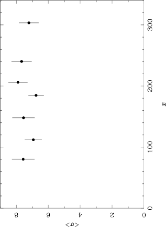
Figure 4: The average rms amplitude ($\sigma=\sqrt{S^{2}}$) as a function of flux for the simulated light curve shown in Fig. 2. The individual rms estimates were sorted by flux and binned to $M=20$ estimates per bin. Errors correspond to the error on the mean value. The amplitude is constant with flux.

5.2.2 Estimating the error on the variance through simulations

The advantage of the above method is that it requires no assumption about the shape of the PSD, The drawback is that it requires a substantial amount of data to produce a single, robust variance estimate. An alternative approach is to estimate the standard deviation of the variances $S_{i}$ based on simulations.

Given an assumed shape for the PSD it is possible to calculate the distribution of variances expected for a stationary process (see section 4.2). Some example distributions are shown in Fig. 3, which clearly demonstrates how the distribution depends on the slope of the PSD. The distribution becomes more normal at flatter slopes and more asymmetric at steep slopes. For a given PSD shape these distributions are well defined (by eqn. 7) and can be computed through Monte Carlo simulations. This makes it possible to estimate limits within which one would expect the variance to be distributed if the process is stationary.

The two primary factors that affect the distribution of variance are the PSD shape and the sampling of the light curve (the length of the data segments in the case of contiguously binned light curves). Table 1 gives the expected confidence limits for four different PSD shapes and five different lengths for the data segments. These values were computed by simulating one very long light curve with the assumed PSD shape and breaking it into $1000$ separate segments (of specified length). The variance within each segment was measured and the distribution of the $1000$ variances was calculated. The $90$ per cent confidence interval was calculated by finding the $5$th and $95$th percentiles of the variance distribution (in general these upper and lower bounds will differ because the distribution is asymmetric). The numbers given in the table are the boundaries of the $90$ and $99$ per cent confidence regions estimated by averaging the results from $50$ runs. The limits are given in terms of $\pm\Delta\log(S^{2})$ because they are multiplicative. That is, from a particular realisation the variance is expected to be scattered within some factor of the true variance (for which the absolute normalisation is irrelevant). The factors are tabulated in terms of their logarithms (since multiplicative factors in linear-space become additive offsets in log-space).

The PSD used for the simulations was chosen to match that expected for AGN, i.e. a steep power-law at high frequencies (with a slope of $\alpha=1.0,1.5,2.0,2.5$) breaking to a flatter slope ($\alpha=1.0$) at low frequencies. The frequency of the break was fixed to be $10^{-3}$, in other words the break timescale was $1000$ times the bin size. (The absolute size of the time bins is arbitrary in the simulations. When comparing the simulated results to real data sampled with e.g. $25$ s time resolution, the break timescale in the simulated PSD is thus $25$ ks.)

Table 1: Expected scatter in variance estimates. The $90$ and $99$ per cent intervals are presented in terms of $\pm\Delta\log(S^{2})$. (The $99$ per cent interval is given in bold.) The boundaries were calculated from Monte Carlo simulations of light curves. The PSD was chosen to be a broken power-law with a slope of $\alpha=1$ below the break (at a frequency $10^{-3}$) and a slope above the break of $\alpha=1.0,1.5,2.0,2.5$. The simulated data segments were chosen to be $10,20,50,100,1000$ points long (the timescale of the break in the PSD being at $1000$, in arbitrary units).

	Number of data points
$\alpha$	10	20	50	100	1000
1.0	-0.84	-0.58	-0.40	-0.32	-0.19
	-0.50	-0.36	-0.26	-0.22	-0.13
	+0.33	+0.28	+0.23	+0.20	+0.15
	+0.53	+0.46	+0.39	+0.35	+0.27
1.5	-0.96	-0.75	-0.62	-0.57	-0.45
	-0.61	-0.50	-0.43	-0.40	-0.32
	+0.39	+0.36	+0.34	+0.33	+0.28
	+0.65	+0.61	+0.58	+0.57	+0.49
2.0	-1.16	-1.01	-0.93	-0.90	-0.72
	-0.78	-0.71	-0.67	-0.66	-0.50
	+0.46	+0.45	+0.44	+0.43	+0.36
	+0.75	+0.73	+0.72	+0.72	+0.59
2.5	-1.49	-1.37	-1.31	-1.28	-0.92
	-1.03	-0.98	-0.95	-0.92	-0.63
	+0.52	+0.52	+0.51	+0.50	+0.40
	+0.83	+0.83	+0.82	+0.80	+0.66

The numbers given in the table provide an approximate prescription for the expected scatter in the variance of a stationary process with a red noise PSD similar to that of AGN. The simulated light curve shown in Fig. 2 was used to demonstrate the use of this table. In this case the PSD is know to have a slope $\alpha=2$, and the variances (shown in panel 3 of Fig. 2) were calculated every $20$ points. Therefore, the $90$ interval for the expected variance is given by $\log(S^{2})_{-0.71}^{+0.45}$. Taking the mean variance as the expectation value for $S^{2}$, this translates to $S^{2}=59.9~{}(11.7-168.8)$. The interval boundaries were calculated by converting the logarithmic value into a linear factor and multiplying by the sample mean (assumed to represent the true variance). This interval is shown on Fig. 5 by the dotted lines. The corresponding $99$ per cent confidence interval is also marked.

Figure 5: Variance of the simulated data shown in Fig. 2 (panel 3) with the $90$ (dotted line) and $99$ per cent (dashed line) confidence intervals marked (as calculated in section 5.2.2). Clearly the variances fall within these limits, as expected for a stationary process. The solid line marks the mean variance.

As expected the individual variances fall within the expected region. However, the $90$ per cent region spans an order of magnitude in variance. Thus even order of magnitude differences in variance between short sections of a light curve are to be expected and do not necessarily indicate that the underlying process is not stationary. Subtle changes in the PSD will thus be difficult to detect by examining the raw variances as the intrinsic scatter is so large. Such changes could be revealed by comparing averaged variances or comparing the PSDs as described above.

6 Effect of measurement errors

6.1 Excess variance and $F_{\rm var}$

The datasets considered thus far have been ideal, in the sense that they are free from flux uncertainties. In real life, however, a light curve $x_{i}$ will have finite uncertainties $\sigma_{{\rm err},i}$ due to measurement errors (such as Poisson noise in the case of an X-ray photon counting signal). These uncertainties on the individual flux measurements will contribute an additional variance. This leads to the use of the ‘excess variance’ (Nandra et al. 1997; Edelson et al. 2002) as an estimator of the intrinsic source variance. This is the variance after subtracting the contribution expected from measurement errors

$$\sigma_{\rm{XS}}^{2}=S^{2}-\overline{\sigma_{\rm{err}}^{2}},$$ (8)

where $\overline{\sigma_{\rm{err}}^{2}}$ is the mean square error

$$\overline{\sigma_{\rm{err}}^{2}}=\frac{1}{N}\sum_{i=1}^{N}\sigma_{{\rm err},i}^{2}.$$ (9)

The normalised excess variance is given by $\sigma_{\rm{NXS}}^{2}=\sigma_{\rm{XS}}^{2}/\bar{x}^{2}$ and the fractional root mean square (rms) variability amplitude ($F_{\rm{var}}$; Edelson, Pike & Krolik 1990; Rodriguez-Pascual et al. 1997) is the square root of this, i.e.

$$F_{\rm{var}}=\sqrt{\frac{S^{2}-\overline{\sigma_{\rm{err}}^{2}}}{\bar{x}^{2}}}.$$ (10)

The statistic $F_{\rm var}$ is often chosen in preference to $\sigma_{\rm NXS}^{2}$ although the two convey exactly the same information. $F_{\rm var}$ is a linear statistics and can therefore give the rms variability amplitude in per centage terms. The choice of whether to quote $F_{\rm var}$ or $\sigma_{\rm NXS}^{2}$ is usually purely one of presentation. It is worth noting that the Monte Carlo results given in section 5.2.2, to estimate the expected scatter on the variance, can also be applied to its square root. The expected boundaries of the confidence region of the logarithm of the rms is approximately half those of the variance. Specifically, $\Delta\log(\sigma)\approx\Delta\log(S^{2})/2$ and similarly $\Delta\log(F_{\rm var})\approx\Delta\log(\sigma_{\rm NXS}^{2})/2$.

6.2 Spectral variability

An X-ray light curve of an AGN can be split into different energy bands. The light curves in each band will be strictly simultaneous and can be used to test whether the X-ray variability is a function of energy. For example, one might examine the ratio of a soft band light curve to a hard band light curve. The statistical significance of any variations in the ratio can be quantified by propagating the measurement errors and applying an appropriate test, such as the $\chi^{2}$ test of the constant ratio hypothesis. If the ratio shows variations greater than those expected from the errors then the two light curves are intrinsically different and the source does indeed show spectral variability. Such changes in the energy spectrum with time can in principle provide valuable clues to the nature of the X-ray source. This test does not provide any quantitative description of the spectral variability.

Another tool for investigating spectral variability is the rms spectrum, i.e. the rms variability amplitude (or $F_{\rm var}$) as a function of energy. See e.g. Inoue & Matsumoto (2001), Edelson et al. (2002), Fabian et al. (2002) and Schurch & Warwick (2002) for some examples of rms spectra from AGN. However, when examining rms spectra it is often not clear whether changes in the amplitude with energy reflect real energy-dependence of the intrinsic variability amplitude or are caused by random errors in the light curves. The finite measurement errors on the individual fluxes (e.g. due to Poisson noise) will introduce some uncertainty in the estimated rms amplitudes. An estimate of this uncertainty would help answer the question posed above, namely whether features in rms spectra are the result of random errors in the data or represent spectral variations intrinsic to the source.

The problem of how to assess the uncertainty on the excess variance (or $F_{\rm var}$) is a long-standing one (e.g. Nandra et al. 1997; Turner et al. 1999; Edelson et al. 2002). The standard error formulae presented in the literature (e.g. Turner et al. 1999; Edelson et al. 2002) are formally valid in the case of un-correlated Gaussian processes. Typically AGN light curves at different X-ray energies are strongly correlated and are not Gaussian. However, when searching for subtle differences in amplitude between simultaneous and correlated light curves it may be more useful to have an indication of the uncertainty resulting from the finite flux errors.

6.2.1 Uncertainty on excess variance due to measurement errors

A Monte Carlo approach was used to develop a prescription of the effect of measurement errors on estimates of $F_{\rm var}$ (and $\sigma_{\rm{NXS}}^{2}$). A short red noise light curve was generated. Poisson noise was added (i.e. the individual flux measurements were randomised following the Poisson distribution) and the excess variance was recorded. The fluxes of the original light curve were randomised again and the excess variance recorded, this was repeated many times. The distribution of excess variances was then used to determine the uncertainty in the variance estimate caused by Poisson noise. Full details of the procedure are given in Appendix B

For these simulations it was found that the error on $\sigma_{\rm{NXS}}^{2}$ decreases as the S/N in the light curve is increased according to:

$$err(\sigma_{\rm{NXS}}^{2})=\sqrt{\left\{\sqrt{\frac{2}{N}}\cdot\frac{\overline{\sigma_{\rm{err}}^{2}}}{\bar{x}^{2}}\right\}^{2}+\left\{\sqrt{\frac{\overline{\sigma_{\rm{err}}^{2}}}{N}}\cdot\frac{2F_{\rm{var}}}{\bar{x}}\right\}^{2}.}$$ (11)

See appendix B for details of this equation and its equivalent in terms of $F_{\rm{var}}$.

As this only accounts for the effect of flux measurement errors (such as Poisson noise) in a given light curve it can be used to test whether two simultaneously observed light curves of the same source, but in different bands, show consistent amplitudes. A demonstration of this using real data is given in the following section. This uncertainty does not account for the random scatter intrinsic to the red noise process, therefore the absolute value of the rms spectrum will change between realisations (i.e. from epoch to epoch). But if a source shows achromatic variability then the values of $F_{\rm{var}}$ calculated in each energy band (at a given epoch) should match to within the limits set by the Poisson noise (i.e. the fractional rms spectrum should be constant to within the uncertainties given by the above equation). Differences in $F_{\rm{var}}$ significantly larger than these would indicate that the source variability amplitude is a function of energy. This would then mean the PSD amplitude/shape is different in different energy bands, or there are multiple spectral components that vary independently.

The above uncertainty estimates can be used to test the hypothesis that the source variability is achromatic. If significant differences between energy bands are detected (as in the case of Mrk 766 presented below) then these errors should not be used to fit the rms spectrum. The assumption that the differences are due only to measurement errors is no longer the case. In such situations the light curves in adjacent energy bands are likely to be partially correlated and so $\chi^{2}$-fitting of the rms spectrum is not appropriate. The differences in excess variance will be a combination of intrinsic differences and measurement errors. Their uncertainty will therefore be more difficult to quantify.

7 Case study: An XMM-Newton observation of Mrk 766

Figure 6: Top panel: 0.2–10.0 keV pn light curve of Mrk 766 (with 25 s bins, in units of ct s^-1). Panel 2 and 3: mean count rate and excess variance measured from segments of 20 points. Panel 4: averaged normalised excess variance measured by binning the individual variance estimates into groups of 20. This average variance is inconsistent with constant. Panel 5: fractional rms amplitude measured from segments of 20 points. Panel 6: averaged fractional rms amplitude measured by binning the individual amplitudes into groups of 20. This average fractional amplitude is consistent with constant. This contrasts with the situation shown in Fig. 2

In this section a long ($\sim 10^{5}$ s) XMM-Newton observation of the bright, variable Seyfert 1 galaxy Markarian 766 is used to illustrate the points discussed above. The data were obtained from the XMM-Newton Data Archive. Details of the observation are discussed in Mason et al. (2003) and an analysis of the PSD is presented in Vaughan & Fabian (2003).

7.1 Observation details

Mrk 766 was observed by XMM-Newton (Jansen et al. 2001) over the period 2001 May 20 – 2001 May 21 (rev. 265). The present analysis is restricted to the data from the pn European Photon Imaging Camera (EPIC), which was operated in small window mode. Extraction of science products from the Observation Data Files (ODFs) followed standard procedures using the XMM-Newton Science Analysis System (SAS) v5.3.3. Source data were extracted from a circular region of radius 35 arcsec from the processed image and only events corresponding to patterns 0–4 (single and double pixel events) were used. Background events were extracted from regions in the small window least effected by source photons, these showed that the background rate increased dramatically during the final $\sim 1.5\times 10^{3}$ s of the observation. This section of the data was excluded, leaving $1.05\times 10^{5}$ s of uninterrupted data. The light curves were corrected for telemetry drop outs (less than 1 per cent of the total time) and background subtracted. The errors on the light curves were calculated by propagating the Poisson noise.

7.2 Stationarity of the data

The broad band (0.2–10 keV) light curve extracted from the pn is shown in Fig. 6 (panel 1). As was the case for the simulated data shown in Fig 2, the mean and variance (calculated every 20 data points) show changes during the length of the observation (panels 2 and 3). The expected range for the excess variance, calculated using the results of section 5.2.2 (and assuming a PSD slope of $\alpha=2.0$), is marked in figure 7. Fig. 8 shows the same data in terms of normalised excess variances. Neither of these show fluctuations larger than expected for a stationary process. But given the large expected scatter this is a rather insensitive test. In the case of the Mrk 766 light curve however, there are sufficient data to examine variations of the average variance with time, allowing a more sensitive test for non-stationarity.

Figure 7: Excess variance of the Mrk 766 data shown in Fig. 6 (panel 3) with the $90$ (dotted line) and $99$ per cent (dashed line) confidence intervals marked (as calculated in section 5.2.2). The variances fall within these limits, as expected for a stationary process. The solid line marks the mean variance.

Figure 8: As for Fig. 7 but using the normalised excess variance of the Mrk 766 data.

By averaging the excess variance estimates (in time bins containing 20 excess variance estimates) significant changes in the variance with time are revealed (panel 4). This contrasts with the simulated data shown in Fig. 2. The binned excess variance is inconsistent with a constant hypothesis: fitting with a constant gave $\chi^{2}=23.1$ for $9$ degrees of freedom ($dof$), rejected at $99$ per cent confidence. The average variance is therefore changing with time, indicating the variability is strongly non-stationary.

Figure 9: Top panel: The average absolute rms amplitude ($\sqrt{\sigma_{\rm XS}^{2}}$) as a function of flux for the Mrk 766  light curve (compare with Fig. 4). Bottom panel: The average  it fractional rms amplitude ($\sqrt{\sigma_{\rm NXS}^{2}}$) as a function of flux. Clearly the absolute rms amplitude is a function of flux, but this dependence is removed in the fractional rms.

A careful inspection of Fig. 6 (panels 3 and 4) shows the individual variance estimates have a tendency to track the source count rate. This is difficult to discern from the individual variances (panel 3), due to the larger intrinsic scatter, but much clearer in the averaged variances (panel 4). This can be seen clearly in Fig. 9 (top panel) where the rms amplitude ($\sqrt{\sigma_{\rm XS}^{2}}$) is shown as a function of count rate. To produce this plot the individual rms estimates (Fig. 6, panel 3) were sorted by count rate and binned by flux (such that there were $20$ estimates per bin). The error on the mean rms was calculated in the standard fashion (see above). This indicates that the source does show a form of genuine non-stationarity: the absolute rms amplitude of the variations increases, on average, as the source flux increases. This effect has been noted in other Seyferts (Uttley & M^cHardy 2001; Edelson et al. 2002; Vaughan et al. 2003) and is due to a linear correlation between rms and flux (see Uttley et al. in prep. for further discussion of this effect). Non-stationarity of this form can be ‘factored out’ by using the normalised amplitude ($F_{\rm var}$ or $\sigma_{\rm NXS}^{2}$) instead of the absolute values. Normalising each variance (or rms) estimate by its local flux removes this trend. The bottom panel of Fig. 9 shows that $F_{\rm var}$ is indeed constant with flux (fitting a constant gave $\chi^{2}=7.8$ for $9~{}dof$). Fig. 6 (panels 5 and 6) shows $F_{\rm var}$ and its average as a function of time; the average is consistent with staying constant ($\chi^{2}=5.8$ for $9~{}dof$). The variability of Mrk 766 does show genuine (strong) non-stationarity, in the sense that the absolute rms increases linearly with flux, but this trend can be removed by using normalised units – $F_{\rm var}$ (and therefore the normalised excess variance) is consistent with being constant (with time and flux).

The above analysis suggests that, after accounting for the effect of the rms–flux correlation, there is no other evidence for strong non-stationarity in the rapid variability of Mrk 766. This was confirmed using the $s$-test of Papadakis & Lawrence (1995; see their Appendix A). A periodogram was calculated for three consecutive segments of $3.4\times 10^{4}$ s duration, and normalised to fractional units (see Appendix A). The $s$ value was computed by comparing periodograms at frequencies below $2\times 10^{-3}$ Hz (above which the Poisson noise power becomes comparable to the source variability). For each pair of periodograms the value of $s$ was within the range expected for stationary data (specifically $\left|s\right|<1$, within one standard deviation of the expected value).

7.3 rms spectrum

The variability amplitude as a function of energy was calculated by measuring $F_{\rm var}$ from light curves extracted in various energy ranges. The results are shown in Fig. 10 and the errors were calculated using equation 16 to account for the effect of Poisson noise. The variability amplitude is clearly a function of energy, i.e. Mrk 766 shows significant spectral variability. This was confirmed by a Fourier analysis of the light curves in different energy bands (Vaughan & Fabian 2003) which revealed complex energy-dependent variability.

The rms spectrum was re-calculated for light curves containing only single pixel (pattern 0) events and again for double pixel (patterns 1–4) events. These two sets of data were extracted from the same detector and using identical extraction regions etc. After accounting for the difference in count rate between single and double pixel events the two sets of light curves should be identical except for the effects of Poisson noise. The two rms spectra should be the same except for Poisson errors. Comparing the ratio of the two rms spectra using a $\chi^{2}$-test (against the hypothesis of unity ratio) gave $\chi^{2}=25.3/20$ degrees of freedom. Comparing the difference of the two rms spectra to the hypothesis of zero difference gave identical results and shows the two rms spectra are indeed fairly consistent. This test indicates that for real data the error formula given above does provide a reasonable description of the uncertainty induced by photon noise.

Figure 10: rms spectrum of Mrk 766 measured using EPIC pn light curves with 1000 s bins.

8 Discussion

The analysis of stochastic processes, such as X-ray variability of AGN, is conceptually different from the analysis of deterministic data such as time-averaged spectra (see discussions in e.g. Jenkins & Watts 1968; Priestley 1981; Bendat & Piersol 1986; Bloomfield 2000). For example, when observing the spectrum of a constant source one expects repeatability of the data to within the limits set by measurement errors, i.e. each new realisation of the spectrum should be consistent within the errors. In AGN variability analysis it is the signal itself that is randomly variable; one does not expected repeatability of quantities such as the mean or variance. These statistical moments will change (randomly) with each new light curve even if there are no measurement errors.

The stochastic nature of red noise processes means that it is usually only their average properties that can provide physical insight. Non-deterministic data should be handled statistically. For example, it is customary to examine the timing properties of X-ray binaries using PSDs estimated from the average periodogram of an ensemble of light curves (e.g. van der Klis 1995). Averaging over many independent realisations reduces the random fluctuations inherent in the noise process.

In most AGN timing studies however there are rarely enough data to construct averages in this way (but see Papadakis & Lawrence 1993 and Uttley et al. 2002 for more on PSD estimation for AGN). As a result of this relative lack of data, AGN timing studies often emphasise the properties of a single light curve. But emphasis on the detailed properties of any single realisation of a stochastic process can be misleading. For example, AGN light curves show large fluctuations in variance. These changes provide little insight as they are expected even when the underlying physical process responsible for the variability is constant. Rather, they may simply be statistical fluctuations intrinsic to the stochastic process. All red noise processes show random fluctuations in both mean and variance and the variance will be distributed in a non-Gaussian fashion with a large scatter (see sections 4.2 and 5).

Previous claims of non-stationary variability based on changes in variance (e.g. Nandra et al. 1997; Dewangan et al. 2002; Gliozzi, Sambruna & Eracleous 2003) should therefore be treated with caution since they did not account for this intrinsic scatter (see also section 3.3.1 of Leighly 1999 for a discussion of this point). Real changes in the PSD would indicate genuine non-stationarity and reflect real changes in the physical conditions of the variability process. Such changes can be measured from the average properties of the light curve, such as the averaged periodogram or the averaged variance (see section 5).

A different issue is that differences between the variance of simultaneous light curves obtained in different energy bands can be examined using the excess variance (or $F_{\rm var}$) statistic. It is possible to estimate the uncertainty in the excess variance due to errors in the flux measurements. This uncertainty, accounting only for measurement (e.g. Poisson) errors, can be used when testing for spectral variability, as demonstrated in section 7.

Estimators such as the excess variance provide a useful, if crude, means of quantifying the variability of AGN. Even though the stochastic nature of AGN light curves makes it difficult to estimate variability amplitudes robustly from short observations, the excess variance can provide useful information. For example an analysis of the excess variances measured from short observations of Seyfert 1 galaxies demonstrated that the variability amplitude (at a given range of timescales) is inversely correlated with the luminosity of the source (Nandra et al. 1997; Leighly 1999; Markowitz & Edelson 2001). Although random fluctuations in variance are expected for AGN light curves the range of variances observed is far larger than could be accounted for by this effect alone. Another example is given in section 7.2 when it is demonstrated that the average variance of Mrk 766 is a function of the flux of the source. A similar effect has been observed in X-ray binaries (Uttley & M^cHardy 2001). A discussion of the implications of this result will be given in Uttley et al. in prep.

9 Conclusions

This paper discusses some aspects of quantifying the variability of AGN using simple statistics such as the variance. Various possible uses of these are presented and some possible problems with their significance and interpretation are brought to light. The primary issues are as follows:

1. In order to search for non-stationary variability in an ensemble of short light curves (or short light curve segments) one can test whether the individual variances are consistent with their mean. Two practical methods are presented (sections 5.2.1 and 5.2.2).

2. In the first method the mean variance and its error are calculated at various epochs by binning the individual variance estimates. This is most useful when searching for subtle changes in variability amplitude but requires large datasets (in order that the variance can be sufficiently averaged).

3. In the second method the individual variance estimates are compared with the expected scatter around the mean. The expected scatter is calculated using Monte Carlo simulations of stationary processes. The table gives some examples of the scatter expected for various PSD shapes typical of AGN. This table can therefore be used to provide a ‘quick look’ at whether the observed fluctuations in the variance are larger than expected. One drawback is that, because the intrinsic scatter in the variance is rather large for red noise data, this method is only sensitive to very large changes in the variability amplitude. Another drawback is that one has to assume a shape for the PSD.

4. The excess variance can also be used to quantify how the variance changes as a function of energy (section 6.2). An approximate formula is presented (based on the results of Monte Carlo simulations) that gives the expected error in the excess variance resulting from only observation uncertainties (flux errors such as Poisson noise). This can be used to test for significant differences in variance between energy bands. If the normalised excess variances (or $F_{\rm var}$s) are found to differ significantly between energy bands this implies the PSD is energy dependent and/or there are independently varying spectral components.

5. Possibly the most robust yet practical approach to variability analysis from AGN data is to test the validity of hypotheses using Monte Carlo simulations. This approach has yielded reliable PSD estimates for Seyfert galaxies (Green et al. 1999; Uttley et al. 2002; Vaughan et al. 2003; Markowitz et al. 2003) and has been used to test the reliability of cross-correlation results (e.g. Welsh 1999) amongst other things. Section 3 discusses some methods for simulating red noise data.

Appendix A Periodogram normalisation

The periodogram is calculated by normalising the modulus-squared of the DFT (see equation 2):

$$P(f_{j})=A|DFT(f_{j})|^{2}.$$ (12)

There are a variety of options for the normalisation $A$ used in the literature, each has desirable properties. In the mathematical literature on time series analysis a normalisation of the form $A=2/N$ is standard (e.g. Priestley 1981; Bloomfield 2000). However, this normalisation is generally not used for time series analysis in astronomy because the periodogram then depends on flux of the source and the binning of the time series. Below are listed three of the most commonly used normalisations, which only differ by factors of $\bar{x}$, the mean count rate in cts/s ($A_{\rm abs}=\bar{x}A_{\rm Leahy}=\bar{x}^{2}A_{\rm rms^{2}}$). The factor of two is present in all these normalisations to make the periodogram ‘one sided,’ meaning that integrating over positive frequencies only yields the correct variance.

1. $A_{\rm rms^{2}}=2\Delta T_{\rm samp}/\bar{x}^{2}N$ – defined by van der Klis (1997) (see also Miyamoto et al. 1991). This is the normalisation most often used in analysis of AGN and X-ray binaries because the integrated periodogram yields the fractional variance of the data. The units for the periodogram ordinate are (rms/mean)² Hz^-1 (where rms/mean is the dimensionless quantity $F_{\rm{var}}$), or simply Hz^-1.

   If a light curve consists of a binned photon counting signal (and in the absence of other effects such as detector dead-time) the expected Poisson noise ‘background’ level in its periodogram is given by

   $$P_{\rm noise}=\frac{2(\bar{x}+B)}{\bar{x}^{2}}\frac{\Delta T_{\rm samp}}{\Delta T_{\rm bin}},$$ (13)

   where $\bar{x}$ is the mean source count rate, $B$ is the mean background count rate, $\Delta T_{\rm samp}$ is the sampling interval and $\Delta T_{\rm bin}$ is the time bin width. The factor of $\Delta T_{\rm samp}/\Delta T_{\rm bin}$ accounts for aliasing of the Poisson noise level if the original photon counting signal contained gaps. If the light curve is a series of contiguous time bins (i.e. $\Delta T_{\rm bin}=\Delta T_{\rm samp}$) and has zero background (which is approximately true for many XMM-Newton light curves of AGN) then this reduces to $P_{\rm noise}=2/\bar{x}$.

   For a light curve with Gaussian errors $\sigma_{{\rm err},i}$ the noise level in the periodogram is

   $$P_{\rm noise}=\frac{2\Delta T_{\rm bin}\overline{\sigma_{\rm{err}}^{2}}}{\bar{x}^{2}}\frac{\Delta T_{\rm samp}}{\Delta T_{\rm bin}}.$$ (14)

2. $A_{\rm Leahy}=2\Delta T_{\rm samp}/\bar{x}N$ – originally due to Leahy et al. (1983). This has the property that the expected Poisson noise level is simply 2 (for continuous, binned photon counting data). If the light curve consists only of Poisson fluctuations then the periodogram should be distributed exactly as $\chi_{2}^{2}$. It is this property that makes this normalisation the standard for searching for periodic signals in the presence of Poisson noise (see Leahy et al. 1983). If the input light curve is in units of ct s^-1 then the periodogram ordinate is in units of ct s^-1 Hz^-1.

3. $A_{\rm abs}=2\Delta T_{\rm samp}/N$ – this is the normalisation used in equation 2. This gives the periodogram in absolute units [e.g. (ct s^-1)² Hz^-1] and so the integrated periodogram gives the total variance in absolute units [e.g. (ct s^-1)²] For a contiguously binned light curve with Poisson errors the noise level is $P_{\rm noise}=2\bar{x}$, and for Gaussian errors the noise level is $P_{\rm noise}=2\Delta T_{\rm bin}\overline{\sigma_{\rm{err}}^{2}}$.

Appendix B Monte Carlo demonstration of Poisson noise induced uncertainty on excess variance

To estimate the effect on $\sigma_{\rm{NXS}}^{2}$ due only to Poisson noise the basic strategy was as follows.

1. Generate a random red noise light curve. This acts as the ‘true’ light curve of the source.

2. Add Poisson noise, i.e. draw fluxes from the light curve according to the Poisson distribution. This simulates ‘observing’ the true light curve. Error bars were assigned based on the ‘observed’ counts in each bin ($\sqrt{counts}$).

3. Measure the normalised excess variance $\sigma_{\rm{NXS}}^{2}$ of the observed light curve. This will be different from the variance of the true light curve because of the Poisson noise.

Steps 2 and 3 were repeated, using the same true light curve, to obtain the distribution of $\sigma_{\rm{NXS}}^{2}$. Fig. 11 shows some results. In this example the ‘true’ light curve was generated with a $f^{-2}$ PSD and normalised to a pre-defined mean and variance, e.g. $S^{2}/\bar{x}^{2}=0.04$ ($F_{\rm{var}}=20$%). This light curve was then observed (i.e. steps 2 and 3 were repeated) $10^{4}$ times. The three panels correspond to different mean count rates for the true light curve (i.e. different S/N of the observation). The ($1\sigma$) widths of the $\sigma_{\rm{NXS}}^{2}$ distributions are Monte-Carlo estimates of the size of the error bars on $\sigma_{\rm{NXS}}^{2}$ due to Poisson noise.

As is clear from Fig. 11 the distribution of $\sigma_{\rm{NXS}}^{2}$ becomes narrower, i.e. the error on $\sigma_{\rm{NXS}}^{2}$ gets smaller, as the S/N of the data increases. Obviously in the limit of very high S/N data the measured value of $\sigma_{\rm{NXS}}^{2}$ will tend to the ‘true’ value (in this case $0.04$), i.e. $err(\sigma_{\rm{NXS}}^{2})\rightarrow 0$ as $counts\rightarrow\infty$. It should also be noted that the distributions are quite symmetrically centred on the correct value, indicating that $\sigma_{\rm{NXS}}^{2}$ is an unbiased estimator of the intrinsic variance in the light curve, even in relatively low S/N data.

In order to assess how the error on $\sigma_{\rm{NXS}}^{2}$ changes with S/N, the width of its distribution was measured from simulated data at various different settings of S/N and intrinsic variance (i.e. $S^{2}/\bar{x}^{2}$). Width of the distribution at each setting was calculated from only $500$ ‘observations’ of each light curve. In order that no particular realisation adversely affect the outcome, and to increase the statistics, this was repeated for $20$ different random light curves (of the same fractional variance) and the width of the $\sigma_{\rm{NXS}}^{2}$ distributions were averaged (i.e. the whole cycle of steps 1–3 was repeated $20$ times). Thus for each specified value of S/N and fractional variance, the error on $\sigma_{\rm{NXS}}^{2}$ is estimated from $10^{4}$ simulated ‘observations.’ These Monte Carlo estimated errors on the normalised excess variance are shown in Fig. 12.

Figure 11: Distribution of measured $\sigma_{\rm{NXS}}^{2}$ from 10,000 ‘observations’ of the same light curve. In each case the ‘true’ $\sigma_{\rm{NXS}}^{2}$ is 0.04 (dotted line). The top panel used the lowest S/N data, the bottom panel used the highest S/N data. The mean number of counts per bin in the simulated light curves was 15 (top), 30 (middle) and 100 (bottom). As the S/N increases (count rate increases) the distribution of $\sigma_{\rm{NXS}}^{2}$ becomes narrower. (Note: this is different from Fig. 3, which shows how the variance changes between different realisations of the same stochastic process.)

Figure 12: Width of the distribution of $\sigma_{\rm{NXS}}^{2}$ (resulting from Poisson noise) as a function of the number of counts per bin. Compare with Fig. 11. The solid curve shows the function described in the text (equation 11).

The solid lines show the functions defined by equation 11 (which was obtained by fitting various trial functions to the Monte Carlo results). Clearly this equation gives a very good match to the Monte Carlo results.

If the variability is not well detected, either because the S/N is low or the intrinsic amplitude is weak, then $S^{2}\approx\overline{\sigma_{\rm{err}}^{2}}$. It is the first term on the right hand side of equation 11 that dominates. If the variability is well detected, i.e. $S^{2}\gg\overline{\sigma_{\rm{err}}^{2}}$, then it is the second term that dominates.

$$err(\sigma_{\rm{NXS}}^{2})\approx\left\{\begin{array}[]{r@{\quad:\quad}l}\sqrt{\frac{2}{N}}\cdot\frac{\overline{\sigma_{\rm{err}}^{2}}}{\bar{x}^{2}}&S^{2}\approx\overline{\sigma_{\rm{err}}^{2}}\vspace{0.2 cm}\\ \sqrt{\frac{\overline{\sigma_{\rm{err}}^{2}}}{N}}\cdot\frac{2F_{\rm{var}}}{\bar{x}}&S^{2}\gg\overline{\sigma_{\rm{err}}^{2}}.\end{array}\right.$$ (15)

In the former case the deviations from the mean are dominated by the errors and the fluxes are approximately normally distributed. In this regime the error equation becomes the same as that given in equation A9 of Edelson et al. (2002). In the latter case the deviations in the light curve are enhanced by the intrinsic variance. The second term is similar to the first except multiplied by a factor $\sqrt{2\sigma_{\rm XS}^{2}/\overline{\sigma_{\rm err}^{2}}}$ to account for this.

Equation 11 can be used to give the uncertainty on $F_{\rm{var}}$ thusly

$$err(F_{\rm{var}})=\frac{1}{2F_{\rm{var}}}err(\sigma_{\rm{NXS}}^{2})=$$

$$\qquad\sqrt{\left\{\sqrt{\frac{1}{2N}}\cdot\frac{\overline{\sigma_{\rm{err}}^{2}}}{\bar{x}^{2}F_{\rm{var}}}\right\}^{2}+\left\{\sqrt{\frac{\overline{\sigma_{\rm{err}}^{2}}}{N}}\cdot\frac{1}{\bar{x}}\right\}^{2}},$$ (16)

and this is the equation used to derive the errors shown in Fig. 10. In the two regimes this becomes:

$$err(F_{\rm{var}})\approx\left\{\begin{array}[]{r@{\quad:\quad}l}\sqrt{\frac{1}{2N}}\cdot\frac{\overline{\sigma_{\rm{err}}^{2}}}{\bar{x}^{2}F_{\rm{var}}}&S^{2}\approx\overline{\sigma_{\rm{err}}^{2}}\vspace{0.2 cm}\\ \sqrt{\frac{\overline{\sigma_{\rm{err}}^{2}}}{N}}\cdot\frac{1}{\bar{x}}&S^{2}\gg\overline{\sigma_{\rm{err}}^{2}}.\end{array}\right.$$ (17)

In the first instance, when the variability is not well detected, $\sigma_{\rm{NXS}}^{2}$ should be preferred over $F_{\rm{var}}$ as negative values of $\sigma_{\rm{NXS}}^{2}$ are possible. Additional Monte Carlo simulations confirmed the above equations are valid for both Gaussian and Poisson distributed flux errors. It is worth reiterating that this error accounts only for measurement errors on the fluxes. It does not account for the intrinsic scatter in the fluxes inherent in any red noise process.

References

- [1] Belloni T., Hasinger G., 1990, A&A, 227, L33
- [2] Belloni T., Psaltis D., van der Klis M., 2002, ApJ, 572, 392
- [3] Bendat J. S., Piersol A. G., 1986, Random Data: Analysis and Measurement Procedures, Wiley (New York)
- [4] Bevington P. R., Robinson D. K,. 1992, Data Reduction and Error Analysis for the Physical Sciences, McGraw-Hill (New York)
- [5] Bloomfield P, 2000, Fourier Analysis of Time Series, Wiley (New York)
- [6] Deeming T. J., 1970, AJ, 75, 1027
- [7] Deeming T. J., 1975, Ap&SS, 36, 137
- [8] Deeter J. E., Boynton P. E., 1982, ApJ, 261, 337
- [9] Dewangan G. C., Boller Th., Singh K. P., Leighly K. M., 2002, A&A, 390, 65
- [10] Done C., Madejski G. M., Mushotzky R. F., Turner T. J., Koyama K., Kunieda H., 1992, ApJ, 400, 138
- [11] Edelson R., Pike G. F., Krolik J. H., 1990, ApJ, 359, 86
- [12] Edelson R., Nandra K. 1999, ApJ, 514, 682
- [13] Edelson R. et al. 2002, ApJ, 568, 610
- [14] Fabian A. C. et al. 2002, MNRAS, 335, L1
- [15] Green A. R., McHardy I. M., Lehto H. J. 1993, MNRAS, 265, 664
- [16] Green A. R., McHardy I. M., Done C., 1999, MNRAS, 305, 309
- [17] Gliozzi M., Sambruna R. M., Eracleous M., 2003, ApJ, 584, 176
- [18] Inoue, H., Matsumoto, C., 2001, AdSpR, 28, 445
- [19] Jenkins G. M., Watts, D. G., 1968, Spectral Analysis and its Applications, Holden-Day (San Fancisco)
- [20] Lawrence A., Watson M. G., Pounds K. A., Elvis M., 1987, Nature, 325, 694
- [21] Lawrence A., Papadakis I., 1993, ApJ, 414, L85
- [22] Leahy D. A., Darbro W., Elsner R. F., Weisskopf M. C., Kahn S., Sutherland P. G., Grindlay J. E., 1983, ApJ, 266, 160
- [23] Lehto H. J., 1989, in J. Hunt, B. Battrick, eds, Two Topics in X Ray Astronomy, (ESA SP-296; Noordwijk: ESA), p499
- [24] Leighly K., 1999, ApJS, 125, 297
- [25] Markowitz A., Edelson R., 2001, ApJ, 547, 684
- [26] Markowitz A. et al. 2003, ApJ, in press (astro-ph/0303273)
- [27] Mason K. O., et al. 2003, ApJ, 582, 95
- [28] McHardy I. M., 1989, in J. Hunt, B. Battrick, eds, Two Topics in X Ray Astronomy, (ESA SP-296; Noordwijk: ESA), p1111
- [29] Nandra K., George I. M., Mushotzky R. F., Turner T. J., Yaqoob T., 1997, ApJ, 476, 70
- [30] Papadakis I. E., Lawrence A., 1993, MNRAS, 261, 612
- [31] Papadakis I. E., Lawrence A., 1995, MNRAS, 272, 161
- [32] Pottschmidt K., 2002, A&A, submitted (astro-ph/0202258)
- [33] Press W. H. 1978, Comments on Astrophysics, 7, 103
- [34] Press W. H., Teukolsky S. A., Vetterling W. T., Flannery B. P., 1996, Numerical Recipes, Cambridge Univ. Press. (Cambridge)
- [35] Press W. H., Rybicki G. B., 1997, in Astronomical Time Series, D. Maoz, A. Sternberg, E. M. Leibowitz (eds.), Kluwer (Dordrecht), p61
- [36] Priestley M. B., 1981, Spectral Analysis and Time Series, Academic Press (London)
- [37] Rodriguez-Pascual P. M. et al. , 1997, ApJS, 110, 9
- [38] Scargle J. D., 1981, ApJS, 45, 1
- [39] Schurch N. J., Warwick R. S., 2002, MNRAS, 334, 811
- [40] Stella L., Arlandi E., Tagliaferri G., Israel G. L., 1997, in ‘Applications of Time Series Analysis in Astronomy and Meteorology’, T. Subba Rao, M. B. Priestley, O. Lessi (eds.), Chapman & Hall (London) (astro-ph/9411050)
- [41] Timmer J., König M. 1995, A&A, 300, 707
- [42] Turner T. J., George I. M., Nandra K., Turcan D., 1999, ApJ, 524, 667
- [43] Uttley P., McHardy I. M., 2001, MNRAS, 323, 26
- [44] Uttley P., McHardy I. M., Papadakis, I. 2002, MNRAS, 332, 231
- [45] van der Klis M., 1989, in Timing Neutron Stars, H. Ogelman, E. P. J. van den Heuvel (eds.), Kluwer (Dordrecht), NATO ASI Series C 262, p27
- [46] van der Klis M., 1995, in X-ray Binaries, W. H. G. Lewin, J. van Paradijs, E. P. J. van den Heuvel (eds.), Cambridge Univ. Press (Cambridge), p252
- [47] van der Klis M., 1997, in Statistical Challenges in Modern Astronomy II, ed. G.J. Babu, E.D. Feigelson, Springer-Verlag (New York), p321
- [48] Vaughan S., Fabian A. C., Nandra K. 2003, 339, 1237
- [49] Vaughan S., Fabian A. C., 2003, MNRAS, 341, 496
- [50] Welsh W. F., 1999, PASP, 111, 1347