Quantitative Interpretation of Quasar Microlensing Light Curves

Abstract

We develop a general method for analyzing the light curves of microlensed quasars and apply it to the OGLE light curves of the four-image lens Q2237+0305. We simultaneously estimate the effective source velocity, the average stellar mass, the stellar mass function, and the size and structure of the quasar accretion disk. The light curves imply an effective source plane velocity of $10200~{}\hbox{km/s}\mathrel{\raise 1.29167pt\hbox{$<$}\mkern-14.0mu\lower 2.58334pt\hbox{$\sim$}}v_{e}h\langle M/M_{\odot}\rangle^{-1/2}\mathrel{\raise 1.29167pt\hbox{$<$}\mkern-14.0mu\lower 2.58334pt\hbox{$\sim$}}39600$ km/s (68% confidence). Given an independent estimate for the source velocity, found by combining estimates for the peculiar velocity of the lens galaxy with its measured stellar velocity dispersion, we obtain a mean stellar mass of $\langle M\rangle\simeq 0.037h^{2}M_{\odot}$ ($0.0059h^{2}M_{\odot}\mathrel{\raise 1.29167pt\hbox{$<$}\mkern-14.0mu\lower 2.58334pt\hbox{$\sim$}}\langle M\rangle\mathrel{\raise 1.29167pt\hbox{$<$}\mkern-14.0mu\lower 2.58334pt\hbox{$\sim$}}0.20h^{2}M_{\odot}$). We were unable to distinguish a Salpeter mass function from one in which all stars had the same mass, but we do find a strong lower bound of $\kappa_{*}/\kappa\mathrel{\raise 1.29167pt\hbox{$>$}\mkern-14.0mu\lower 2.58334pt\hbox{$\sim$}}0.5$ on the fraction of the surface mass density represented by the microlenses. Our models favor a standard thin accretion disk model as the source structure over a simple Gaussian source. For a face-on, thin disk radiating as a black body with temperature profile $T_{s}\propto R^{-3/4}$, the radius $r_{s}$ where the temperature matches the filter pass band (2000Å or $T_{s}(r_{s})\simeq 7\times 10^{4}$ K) is $1.4\times 10^{15}h^{-1}\hbox{cm}\mathrel{\raise 1.29167pt\hbox{$<$}\mkern-14.0mu\lower 2.58334pt\hbox{$\sim$}}r_{s}\mathrel{\raise 1.29167pt\hbox{$<$}\mkern-14.0mu\lower 2.58334pt\hbox{$\sim$}}4.5\times 10^{15}h^{-1}\hbox{cm}$. The flux predicted by the disk model agrees with the observed flux of the quasar, so non-thermal or optically thin emission processes are not required. From the disk structure we estimate a black hole mass of $M_{BH}\simeq 1.1_{-0.7}^{+1.4}\times 10^{9}h^{-3/2}\eta_{0.1}^{1/2}(L/L_{E})^{-1/2}M_{\odot}$, consistent with the mass estimated under the assumption that the quasar is radiating at the Eddington luminosity ($L/L_{E}=1$).

1 Introduction

The term “microlensing” describes the flux variations produced in a background source by foreground stars in two very different regimes. Today, astronomers are most familiar with the local (Galactic) phenomenon, in which a star or binary produces a time variable magnification of a background star (see the reviews by Paczynski Paczynski96 (1996) or Mao Mao01 (2001)). Because the physical distances are so short, the Galaxy is optically thin to microlensing ($\tau\sim 10^{-6}$). This leads to the disadvantage that few background sources are lensed (one in $\tau^{-1}$ stars), and the advantage that the lens producing the variations is simple (one or two isolated stars). In quasar microlensing, by contrast, the existence of multiple quasar images requires a microlensing optical depth near unity ($\tau\sim 1$) if the stars in the lens galaxy are a significant fraction of the surface density (see the review by Wambsganss Wambsganss01 (2001)). This regime has the advantage that all background sources are microlensed, but the disadvantage that the lens is intrinsically complex, as it consists of a star field rather than a star.

In either experiment, the light curve of the background source provides a time history of the changes in the magnification created by the relative motions of the observer, the source, and the lens. At its simplest, these variations determine a time scale, $\Delta t\propto M^{1/2}v_{e}^{-1}x^{1/2}(1-x)^{1/2}$, set by the mass $M$, the effective source velocity $v_{e}$, and the fractional distance $x$ of the lens from the source. These scalings are exact for Galactic microlensing events, and the stellar mass can be inferred only from the statistical properties of large samples (e.g. Alcock et al. Alcock00 (2000)) or from events where special circumstances allow an independent determination of $v_{e}$ or $x$ (e.g. parallax effects, Grieger, Kayser & Refsdal Grieger86 (1986), Gould Gould92 (1992)). For quasar microlensing, these same factors determine the typical time between “events” in which there is a significant change in the magnification, with the advantage that the fractional distance $x$ is known from the redshifts, leaving only a degeneracy between the mass and velocity scales. If the fundamental physics probed by the two regimes is the same, why has the astronomical community devoted far more observational resources to Galactic microlensing than to extragalactic microlensing?

The first problem is that the time scales for quasar microlensing are roughly ten times longer than for Galactic microlensing, because the larger length scales of the extragalactic regime are only partly balanced by the larger velocity scales. As a result, “events” take 1–10 years rather than 0.1–1 years. This is no longer a viable argument for ignoring quasar microlensing. There are roughly 40 multiply-imaged quasars that could be monitored, with a total of roughly 120 images, so that even if the “event” rate is only one per image per decade, there are 10 quasar microlensing “events” occurring each year. Quasar microlensing requires less intensive monitoring because of the longer time scales (once per week rather than once per day), so a total of roughly 2000 images/year is needed to monitor the available lens sample. Even with the addition of more intensive monitoring during events, this represents a small fraction of the effort in a large Galactic microlensing survey.

The second problem is that the quasar images are separated by only arcseconds, making it difficult to obtain the independent image fluxes. Fortunately, many telescopes routinely produce sub-arcsecond resolution images. When combined with difference imaging (e.g. Alard Alard00 (2000)) to compensate for PSF variations with epoch and to remove the non-varying components of the lens, and accurate astrometry and component parameters from HST images (e.g. Lehar et al. Lehar00 (2000)), it is now relatively easy to produce light curves. Arguably the best light curve available for quasar microlensing was produced by the Optical Gravitational Lens Experiment (OGLE) using the same observing procedures as for their primary Galactic microlensing experiment, combined with difference imaging to analyze the results (Wozniak et al. 2000a , 2000b ).

The third problem is that we can never observe the “unlensed” source to get a baseline from which to determine absolute magnifications. This problem is no worse than the blending problem for Galactic microlenses, in which the flux of the lensed star is contaminated by flux from a nearby star (Di Stefano & Esin DiStefano95 (1995)) or many unresolved stars (pixel lensing, Crotts Crotts92 (1992)). It is certainly true that there is no means of determining the absolute magnifications of the individual images because this is degenerate with the unknown flux of the quasar. However, by taking advantage of the spatial structure of quasars, it is possible to determine the true magnification ratios between the images in the absence of microlensing. The emission line, mid-infrared and radio emitting regions of quasars should all be large enough to average out the effects of microlensing to allow the determination of the “intrinsic” flux ratios (e.g. Wyithe et al. 2002a for Q2237+0305).

The fourth problem is that the quasar lenses have sources that are time variable, making it necessary to separate intrinsic and microlensing variability. If the source is time variable and contaminating the microlensing flux variations, then the light curves can be used to determine the time delay between the images and the effects of the intrinsic variability are eliminated by comparing the light curves shifted by the time delay. Moreover, the time delay measurement provides a direct estimate of the total surface density near the lensed images (under the assumption that $H_{0}$ is known, see Kochanek Kochanek02 (2002)), which can be compared to the estimates of the total or stellar surface density derived from analyzing the variability created by microlensing. If the source is not variable, or the time delay is short compared to the microlensing time scales, then it is unimportant for understanding the microlensing.

The fifth, and most significant problem, is the difficulty in interpreting the quasar microlensing light curves. Even the complex light curves produced by binary lenses (e.g. Mao & Paczynski Mao91 (1991)), are far simpler than those produced by the collective effects of many stars. The first observational studies of quasar microlensing used semi-quantitative analyses of the temporal widths of light curve peaks to estimate the size of the accretion disk in the source quasar of Q2237+3035 (e.g. Webster et al. Webster91 (1991), Wambsganss, Paczynski & Schneider Wambsganss90 (1990), Rauch & Blandford Rauch91 (1991)). More recent studies of the source structure focused on detailed analyses of “high magnification events,” where the magnification pattern should have the generic asymptotic properties of a fold or cusp caustic (e.g. Yonehara Yonehara01 (2001), Shalyapin et al. Shalyapin02 (2002)). General analyses of light curves have focused on estimates of their statistical properties. In particular, Seitz & Schneider (Seitz94a (1994)), Seitz, Wambsganss & Schneider (Seitz94b (1994)) and Lewis & Irwin (Lewis96 (1996)) considered the auto-correlation functions of light curves, Wyithe, Webster & Turner (Wyithe99 (1999)) considered the distributions of light curve derivatives, and Lewis & Irwin (Lewis95 (1995)) considered the probability distributions of the magnifications. In all cases, the application of these statistical methods has been to the four-image lens Q2237+0305 (Huchra et al. Huchra85 (1985)) in order to estimate the average microlens mass (e.g. Refsdal & Stabell Refsdal93 (1993), Seitz et al. Seitz94b (1994), Lewis & Irwin Lewis96 (1996), Wyithe et al. 2000c ), the transverse velocity (Wyithe & Turner Wyithe01 (2001)), and the source size and structure (e.g. Witt & Mao 1994a , Wyithe et al. 2000e , Wyithe, Agol & Fluke 2002a ). While these are reasonable statistical estimators, they are difficult to apply to irregularly sampled, sparse data and they lose information compared to the raw light curves because the statistics of the light curves are highly non-Gaussian. The biggest problem in using quasar microlensing for astrophysics remains the problem of interpreting the data.

While many of the astrophysical applications of Galactic and quasar microlensing analyses are similar, there is a fundamental difference in using the two methods to study the dark matter problem. In quasar microlensing, the behavior of the light curves depends on both the density of the stars and the density of the smoothly distributed matter. Moreover, the effects of the two density components can be distinguished (e.g. Schechter & Wambsganss Schechter02 (2002)). Simple studies of the dependence of image flux ratios on image parities already suggest that in most quasar lenses the stars must represent only a modest fraction of the total density (see Schechter & Wambsganss Schechter02 (2002), Kochanek & Dalal Kochanek03 (2003)). This is very different from Galactic microlensing experiments which, even with infinite resources, can only determine the density of the halo in compact objects (stars, planets etc.). The inference that the rest of the halo must be composed of smoothly distributed (particle) dark matter comes only from comparing the measured density to that inferred from dynamical studies of the Galaxy. With quasar microlensing, no additional step is required. The greater ability of quasar microlensing to address the dark matter problem makes solving the problem of interpreting the data an important one.

In this paper we develop and demonstrate a method for obtaining physical information from quasar microlensing data of arbitrary complexity and apply it to Q2237+0305. We will simultaneously estimate the source velocities, source size, source structure, stellar mass function and stellar surface density fraction needed to obtain statistically acceptable models of the Q2237+0305 light curves measured by OGLE (Wozniak et al. 2000a , 2000b ). In doing so, we also obtain model light curves that are consistent with the observations. We outline our approach in §2, with additional details on our method of computing microlensing magnification patterns given in Appendix A. Since the distribution of stars needed to reproduce the available data is not unique, we introduce a Bayesian statistical method to estimate any physical variables of interest. In §3 we analyze the OGLE light curves for Q2237+0305 to estimate the source velocity and average stellar mass (§3.1), the source structure (§3.2), the physical properties of the accretion disk and the mass of the black hole (§3.3), the surface density of the stars (§3.4), and the flux ratios of the images (§3.5). In §3.6 we survey some of the best fits to the light curves. Finally, in §4 we summarize the results and outline the potential future of quasar microlensing.

2 A New Approach to Analyzing Quasar Microlensing Data

Just as in the analysis of Galactic microlensing light curves (see Afonso et al. Afonso00 (2000) for a spectacular example), we will analyze quasar microlensing light curves by finding configurations of stars and source trajectories that reproduce the observations. Because the stellar configurations are complex, we search for good fits to the data by producing large numbers of random realizations of the light curves. Then, using a Bayesian analysis of the the goodness of fit statistics for these model light curves, we estimate the values and uncertainties for any physical variable of interest.

We generate source plane magnification patterns using the ray-shooting method (e.g. Schneider et al. Schneider92 (1992)). The technical details of our method, which has a number of non-standard features, are summarized in Appendix A. For our study of Q2237+0305 we used fixed values from lens models for the mean convergence $\kappa$ and shear $\gamma$ at the location of each image, but considered models with a range of stellar mass fractions $\kappa_{*}/\kappa=1$, $1/2$, $1/4$ and $1/8$ where $\kappa_{*}\leq\kappa$ is the surface density of the stars. The stars are distributed randomly in position and are drawn from a power-law mass function $dp/dM\propto M^{-x}$ over a finite mass range $M_{1}<M<M_{2}$. We normalize our length scale by the Einstein radius $\langle\theta_{E}\rangle$ corresponding to the average mass $\langle M\rangle$, and parameterize the mass function by the exponent $x$ and the ratio between the upper and lower masses $r=M_{2}/M_{1}$. In the present calculation we use either a Salpeter mass function ($x=2.35$) with a mass ratio $r=100$, or a “mono-mass” mass function in which all stars have the same mass ($r=1$). Our standard magnification pattern was a square region spanning $40\langle\theta_{E}\rangle$ stored in a $2048^{2}$ array with a pixel scale of $0.02\langle\theta_{E}\rangle$. These scales were chosen so that we could make large numbers of statistically independent trial light curves from a single magnification map.

In Galactic microlensing, stellar angular diameters are much smaller than the lens Einstein radius, so the effects of finite source size are seen only during caustic crossings (e.g. Witt & Mao 1994b ). For quasar microlensing there is less separation of the two scales, making finite source sizes more important (e.g. Kayser, Refsdal & Stabell Kayser86 (1986), Schneider & Weiss Schneider87 (1987)). For a given source model, we convolve the raw magnification pattern with the surface brightness model of the source before computing the light curves. The physical effects of the source size are controlled by the ratio between the source size and the average Einstein radius, $r_{s}/\langle\theta_{E}\rangle\propto r_{s}/\langle M\rangle^{1/2}$, so we assumed circular sources scaled by the average mass of the stars. For length scale $r_{s}=\hat{r}_{s}\langle M/M_{\odot}\rangle^{1/2}$, we computed light curves for scales from $\hat{r}_{s}=10^{15}h^{-1}$ cm (slightly below our pixel scale) to $10^{18}h^{-1}$ cm (somewhat above the average Einstein radius) in steps of $\Delta\log\hat{r}_{s}=0.25$. We used either a Gaussian or a thin disk model for the surface brightness profile $I(R)$. The Gaussian model for the surface brightness,

$$I(R)\propto\exp\left(-R^{2}/2r_{s}^{2}\right)$$ (1)

is the model usually used in microlensing studies. For a comparison, we used a standard model for an optically thick, pressure supported, absorption opacity-dominated, thin accretion disk in which energy is released locally with a black body spectrum (e.g. Shapiro & Teukolsky Shapiro83 (1983)). For a black hole of mass $M_{BH}$ and accretion rate $\dot{M}$, the energy dissipation rate per unit area of the disk, $3GM_{BH}\dot{M}/8\pi R^{3}$, must equal the radiation losses of $\sigma T_{s}^{4}$, so the disk surface temperature $T_{s}\propto R^{-3/4}$. We will not include the correction factor of $1-(3R_{BH}/R)^{1/2}$ to the dissipation rate near the last stable orbit of the black hole so as to avoid additional parameters. For reasonably narrow filters ($\Delta\lambda/\lambda\sim 15\%$ for the V-band) the surface brightness of the disk

$$I(R)\propto\left[\exp\left((R/r_{s})^{3/4}\right)-1\right]^{-1}.$$ (2)

simply tracks the black body spectrum. The scale length $r_{s}$ is the radius at which the disk surface temperature matches the effective wavelength of the filter – for V-band observations of Q2237+0305 (2000Å in the rest frame), the temperature at radius $r_{s}$ is $T_{s}(r_{s})\simeq 70000$ K. The thin disk model can be used to make self-consistent predictions for the wavelength dependence of the microlensing effects because the radius scales with photon wavelength as $r_{s}\propto\lambda^{4/3}$.

The light curves produced by the two models weight the magnification pattern very differently. On small scales, $R<r_{s}$, the Gaussian model has nearly constant surface brightness while the black body model is a centrally peaked power law, $I(R)\sim R^{-3/4}$. On large scales, $R>r_{s}$, the Gaussian model cuts off much more sharply than the black body model. We will consider only circular (face on) disks to avoid introducing two additional parameters for the inclination and orientation of the disk. This means that estimates of the scale length will tend to be underestimates. Crudely, microlensing measures the area of the source rather than the radius, so for circular scale length $r_{s,circ}$ the true scale length $r_{s,true}$ of a disk with axis ratio $q$ is roughly $r_{s,true}\simeq r_{s,circ}/(1-q)^{1/2}$.

Once we have the convolved magnification pattern, we can choose an initial point ${\bf u}_{0}$ and an effective velocity ${\bf v}_{e}=v_{e}\left(\cos\Theta,\sin\Theta\right)$ for the trajectory to compute the magnification as a function of time. We make two simplifications in generating the light curves. First, we neglect the internal motions of the stars in the lens galaxy and use fixed magnification patterns. Studies of the effects of moving stars (e.g. Kundic & Wambsganss Kundic93 (1993), Schramm et al. Schramm93 (1993), Wyithe, Webster & Turner 2000a ) generally found that their effects were difficult to statistically distinguish from a simple, static magnification pattern. Secondly, we regard the trajectory directions ($\Theta$) as independent, uniformly distributed random variables for each image. We experimented with the effects using the same $\Theta$ for all images and found that it had little effect on the results. Moreover, the neglected internal motions of the stars “randomize” the trajectories, making perfectly locked trajectories unphysical without the inclusion of the stellar motions. For each trajectory we compute the change in magnitudes, $\delta\mu^{\alpha}(t)$, produced by microlensing image $\alpha$, relative to the mean magnification for the image.

2.1 Fitting the Data

The data consists of a series of magnitude measurements $m^{\alpha}_{i}$ for image $\alpha$ at epoch $i$ with uncertainties $\sigma_{\alpha,i}$. These magnitudes are a combination of the source magnitude at that epoch $S_{i}$, the local mean magnification for the image $\mu^{\alpha}$ (as a magnitude), any offsets in the magnitude due to extinction, substructure or other systematic effects on the image fluxes $\Delta\mu^{\alpha}$, and the time varying change in the magnification due to microlensing $\delta\mu_{i}^{\alpha}$ relative to the local mean,

$$m^{\alpha}_{i}=S_{i}+\mu^{\alpha}+\Delta\mu^{\alpha}+\delta\mu_{i}^{\alpha}=S_{i}+\mu^{\alpha}_{tot,i}.$$ (3)

We measure the goodness of fit with a $\chi^{2}$ statistic,

$$\chi^{2}=\sum_{\alpha}\sum_{i}\left[{m^{\alpha}_{i}-S_{i}-\mu^{\alpha}_{tot,i}\over\sigma_{\alpha,i}}\right]^{2}.$$ (4)

In addition to the microlensing magnification curves, $\delta\mu_{i}^{\alpha}$, for each image, the model parameters are the source flux $S_{i}$, and the offsets $\Delta\mu^{\alpha}$ from the mean magnification. If there is a significant time delay between the images, then we would need to include the appropriate temporal offsets between the light curves.

The source magnitude must be determined for each individual model since it is not a direct observable. We can do so either by estimating it from the data for each epoch or by assuming a parameterized model for its variation with time. If we estimate it from the data for each epoch, which we will call a “non-parametric” model, we solve $\partial\chi^{2}/\partial S_{i}=0$ to find that

$$S_{i}=\left[\sum_{\alpha}{m^{\alpha}_{i}-\mu^{\alpha}_{tot,i}\over\sigma_{\alpha,i}^{2}}\right]\left[\sum_{\alpha}{1\over\sigma_{\alpha,i}^{2}}\right]^{-1}.$$ (5)

The $\chi^{2}$ statistic then reduces to a sum over the $N(N-1)/2$ possible difference light curves of the $N$ images,

$$\chi^{2}=\sum_{\alpha}\sum_{\beta<\alpha}\sum_{i}\left[{\left(m^{\alpha}_{i}-\mu^{\alpha}_{tot,i}\right)-\left(m^{\beta}_{i}-\mu^{\beta}_{tot,i}\right)\over\sigma_{\alpha\beta,i}}\right]^{2}.$$ (6)

The errors $1/\sigma_{\alpha\beta,i}^{2}$ are the product of the $N-2$ errors excluding images $\alpha$ and $\beta$ divided by the sum of all the exclusive permutations of $N-1$ errors. For example, if we have 4 images labeled A-D, the weighting for the A/B difference light curve is

$${1\over\sigma_{AB,i}^{2}}={\sigma_{C,i}^{2}\sigma_{D,i}^{2}\over\sigma_{A,i}^{2}\sigma_{B,i}^{2}\sigma_{C,i}^{2}+\sigma_{A,i}^{2}\sigma_{B,i}^{2}\sigma_{D,i}^{2}+\sigma_{A,i}^{2}\sigma_{C,i}^{2}\sigma_{D,i}^{2}+\sigma_{B,i}^{2}\sigma_{C,i}^{2}\sigma_{D,i}^{2}}.$$ (7)

While statistically optimal, the actual source behavior can be unphysical if we are confident that the intrinsic variability and microlensing effects have different time scales. For example, suppose image A is crossing a caustic and has a peak, while image B has more or less constant flux. If we have a poor model for the microlensing light curves with a peak at neither A nor B, then the source will be given a peak which is half the amplitude of the observed peak. If we are confident that the source should be varying slowly, then the a priori probability of the source conspiring to mimic part of the microlensing peak is low. We can force the source to show little correlation with shorter time-scale microlensing variability by using a parametric model for the source. For example, a source described by a polynomial $S_{i}=p_{0}+p_{1}t_{i}+p_{2}t_{i}^{2}\cdots$ function of the epoch $t_{i}$ leads to simple linear equations $\partial\chi^{2}/\partial p_{i}=0$ for the source parameters. Parameterized source models also allow us to fit the light curves of one image at a time. In particular, if we assume that the source has a nearly constant magnitude $S_{0}$ with random magnitude fluctuations of $\sigma_{0}$, then we can fit the light curve of a single image as

$$\chi^{2}_{\alpha}=\sum_{i}{\left(m_{i}^{\alpha}-S_{0}-\delta\mu_{i}^{\alpha}\right)^{2}\over\sigma_{\alpha,i}^{2}+\sigma_{0}^{2}}.$$ (8)

Analyzing a single image allows for far more rapid calculations than joint analyses of four images because it avoids the combinatoric explosion we discuss in §2.2. We will call these “parametric” models.

Although there is no theoretical problem with including measurements (e.g. extinction estimates) or constraints (e.g. the relative macro magnifications must be correct to some accuracy) on the magnitude offsets, we decided that for our present study we would use only the time variability of the images to constrain the models. This means that we solve for the optimal value of the offsets, $\Delta\mu^{\alpha}$, for every trial light curve. If our time series is sufficiently long, so that it averages over many Einstein radii of the microlensing pattern, then these estimates of the offsets from fitting the light curves should converge to their true value. Otherwise, they will show significant scatter depending on whether the light curve lies in a region of higher or lower than average microlensing magnification.

2.2 Dealing With The Combinatoric Explosion

The probability of a randomly drawn microlensing magnification curve leading to a reasonable fit to the OGLE light curves is small and we cannot try every possible trajectory for a broad range of physical parameters. For this study we used magnification patterns with an outer scale of $40\langle\theta_{E}\rangle$ and dimensions of $2048\times 2048$ pixels, leading to an inner, pixel scale of $0.02\langle\theta_{E}\rangle$. For a compact source and a light curve with a caustic crossing feature, testing all possible trial light curves for a single pattern, source size and effective velocity would require of order $10^{14}$ trials. If we want study more than one image over a broad range of effective velocities, source sizes and physically different magnification patterns, then we are forced to use Monte Carlo methods to search a random sampling of the trajectories. In practice we find that for fitting a single image of Q2237+0305 assuming a constant source with random intrinsic fluctuations of $\sigma_{0}=0.05$ mag that approximately one in every $N\simeq 100$ trial realizations will produce a fit with $\chi^{2}/N_{dof}\mathrel{\raise 1.29167pt\hbox{$<$}\mkern-14.0mu\lower 2.58334pt\hbox{$\sim$}}3$ where $N_{dof}$ is the number of degrees of freedom. Obviously a much smaller fraction produce fits with $\chi^{2}/N_{dof}\simeq 1$.

The problem explodes when we try to fit more than one light curve simultaneously. Crudely, if we fit 2, 3 or 4 light curves simultaneously we would expect that it would take $N^{2}\simeq 10^{4}$, $N^{3}\simeq 10^{6}$ or $N^{4}\simeq 10^{8}$ trials to produce equally good fits to all the images simultaneously. At least when using the non-parametric method, the scaling is less extreme because there are so many degrees of freedom in the source. In practice, finding a fit for two images using the non-parametric method is not much harder than finding a fit for one image with the simpler parametric method. It is possible to find reasonable four-image solutions in $N\simeq 10^{6}$ trials. We speed the process of finding good realizations in two ways.

First, we set a threshold, $\chi_{max}^{2}$, on the value of the $\chi^{2}$ statistic, and assume that any light curve exceeding this value (and any local perturbations to it) should have zero statistical weight in our analysis. We then note that as we add data points to the determination of a $\chi^{2}$ statistic, the statistic can only increase in absolute value. We take advantage of this by computing the $\chi^{2}$ using the data points in a random temporal order and stopping the calculation as soon as $\chi^{2}>\chi^{2}_{max}$. If we set $\chi^{2}_{max}=3N_{dof}$ (for the parametric models, $5N_{dof}$ for the non-parametric models), then the vast majority of trials light curves are disposed of based on a small fraction of the data points. Because nearby points of both the light curves and the magnification patterns tend to be similar, while well-separated points tend to be dissimilar, random ordering of the data allows much faster rejection of a trial light curve than sequential ordering.

Second, for trial light curves which have $\chi^{2}<\chi^{2}_{max}$, we locally optimize the parameters (the starting points ${\bf u}_{0}$ and the directions at fixed effective velocity $\Theta$) of the curves to minimize the $\chi^{2}$. This step helps considerably in finding good solutions given our inability to try every possible set of initial conditions in our magnification pattern. We get a fair random sampling of the global initial conditions, but allow for a local optimization since we cannot perform the fine sampling needed to try every initial condition. The optimization step means that we need to keep our threshold $\chi^{2}_{max}$ sufficiently high so that typical optimizations of cases above the threshold would not reduce the $\chi^{2}$ to the point where the trials become statistically significant.

There is some risk that these modifications can create biases in the results. For example, in regions with complex caustic structures the source trajectory requires better alignment with the magnification pattern in order to fit the data than in regions with less complex structures. Hence, the combination of an initial threshold followed by local optimization could bias our results against finding solutions in the complex regions. While it was not computationally feasible to conduct our complete model survey without a threshold, we did test specific cases and found no evidence for the procedures introducing a bias.

2.3 Parameter Estimation

We use Bayesian methods for parameter estimation based on comparing large numbers of trial light curves to the observed data. The statistical properties of the light curves expected for each image depend on the local magnification tensor ($\kappa$ and $\gamma$), the local properties of the stars ($\kappa_{*}$, $\langle M\rangle$, $x$ and $r$), the structure of the source (Gaussian or thin disk, $r_{s}$) and the effective velocity of the source ${\bf v}_{e}=v_{e}\left(\cos\Theta,\sin\Theta\right)$. We will collectively refer to these physical parameters as ${\bf\xi_{p}}$. For any given set of physical parameters we generate large numbers of source trajectories described by their starting points (${\bf u}_{0}$) and directions ($\Theta$). We regard these trajectory parameters, which we will collectively refer to as ${\bf\xi_{t}}$, as nuisance parameters that we will project out of the likelihoods.

For each trial light curve we obtain a goodness of fit defined by the $\chi^{2}$ statistics introduced in §2.1. Our next step is to define the relative likelihoods of the light curves given the $\chi^{2}$ values. Using a standard maximum likelihood estimator, like $P(D|{\bf\xi_{p}},{\bf\xi_{t}})=\exp(-\chi^{2}/2)$, works poorly because we are comparing the probabilities of completely different light curves rather than models related to each other by continuous changes of parameters. We would expect even “perfect” model light curves to have $\langle\chi^{2}\rangle\simeq N_{dof}\pm(2N_{dof})^{1/2}$, so only $\chi^{2}$ differences of order $(2N_{dof})^{1/2}$ indicate whether one light curve is superior to another. For this reason we base our likelihoods on the probability of obtaining a given value of $\chi^{2}$ for data with $N_{dof}$ degrees of freedom,

$$P(\chi^{2}|N_{dof})={dP\over d\chi^{2}}\propto\chi^{N_{dof}-2}\exp\left(-\chi^{2}/2\right).$$ (9)

The second problem is that we are fitting data with a large number of degrees of freedom ($N_{dof}=290$ for the simultaneous fits to all four images of Q2237+0305 discussed in §3), so our $\chi^{2}$ estimates are very sensitive to small errors in the magnitude uncertainties of the light curves. It takes only a 4% shift in the magnitude uncertainties to produce a $(2N_{dof})^{1/2}$ change in $\chi^{2}$ when $N_{dof}=290$.

We control this problem by allowing for uncertainties in the magnitude errors $\sigma_{\alpha},i$. If we scale the magnitude errors by the factor $f$, then the value of $\chi^{2}$ changes to $\chi_{f}^{2}=\chi^{2}/f^{2}$ with distribution $P(\chi_{f}^{2}|N_{dof})=P(\chi^{2}/f^{2}|N_{dof})/f^{2}$. By averaging over $f$, weighted by some prior $P(f)$ for our level of uncertainty in the errors, we can obtain estimates for the relative probabilities of the models that are insensitive to errors in the magnitude uncertainties. We set the magnitude errors to be the quadrature sum of the OGLE uncertainties and $0.05$ mag, and found that our best fit models had $\chi^{2}\simeq 200$ for $N_{dof}=290$. This suggests that we overestimated the magnitude errors by at least 20%, and that we can assume $0\leq f\leq 1$. Since the data contains real measurement errors, $P(f)$ must approach zero as $f\rightarrow 0$. For simplicity we adopt $P(f)\propto f$ for $0\leq f\leq f_{0}=1$, in which case the weighted average of $P(\chi^{2}_{f}|N_{dof})$ over $f$ becomes

$$P(\chi^{2})\propto\Gamma\left[{N_{dof}-2\over 2},{\chi^{2}\over 2f_{0}^{2}}\right],$$ (10)

where $\Gamma[a,b]$ is an incomplete Gamma function. This expression has the “correct” properties for estimating the relative probabilities of light curve realizations. First, like the $\chi^{2}$ distribution, light curve realizations must have $\chi^{2}$ differences comparable to $(2N_{dof})^{1/2}$ before they have significantly different relative probabilities. Second, when $\chi^{2}$ is larger than $N_{dof}$, it simply becomes a $\chi^{2}$ distribution set by the maximum plausible error $f_{0}$ and with an unimportant reduction in the number of degrees of freedom. Third, when the $\chi^{2}$ is smaller than $N_{dof}$, the likelihood of the models rises, with $P(0)/P(N_{dof})\simeq 2$, rather than falling as it does for the true $\chi^{2}$ distribution (Eqn. 9). When we find models with $\chi^{2}<N_{dof}$, it is probably because we have overestimated the magnitude errors rather than because we have over fit the data. In summary, the advantage of this likelihood estimator is that it benignly handles the problem of systematic uncertainties in the $\chi^{2}$ estimators even when $N_{dof}$ is large. Our approach is conservative because it will overestimate the uncertainties in any results provided the true errors correspond to the region with $f\leq f_{0}=1$.

Using Bayes’ theorem, the probability of the parameters given the data is

$$P({\bf\xi_{p}},{\bf\xi_{t}}|D)\propto P(D|{\bf\xi_{p}},{\bf\xi_{t}})P({\bf\xi_{p}})P({\bf\xi_{t}})$$ (11)

where $P({\bf\xi_{p}})$ and $P({\bf\xi_{t}})$ describe the prior probability estimates for the physical and trajectory variables respectively, and $P(D|{\bf\xi_{p}},{\bf\xi_{t}})=P(\chi^{2})$ as defined in Eqn. 10. All Bayesian parameter estimates are normalized by the requirement that the total probability is unity, $\int d{\bf\xi_{p}}d{\bf\xi_{t}}P({\bf\xi_{p}},{\bf\xi_{t}}|D)=1$. We assume that the trajectory starting points and directions are uniformly distributed and that they are nuisance variables. We obtain the probability distributions for the more interesting statistical parameters by marginalizing over the trajectory variables

$$P({\bf\xi_{p}}|D)\propto\int P({\bf\xi_{p}},{\bf\xi_{t}}|D)d{\bf\xi_{t}}.$$ (12)

In practice we sum the probabilities for our random sampling of trajectories, which is equivalent to using Monte Carlo integration methods to compute the integral over the space of all possible trajectories. The sum over the random trajectories will converge to the true integral provided we make enough trials.

For our present study we assumed that the values of $\kappa$ and $\gamma$ are known exactly from lens models. We studied a range of values for the fraction of the surface density composed of stars with a logarithmic prior $P(\kappa_{*})\propto 1/\kappa_{*}$. We considered discrete trials of the different mass function parameters ($x$ and $r$) and the two source structures with all the cases given equal prior likelihoods. We used a logarithmic prior $P(\hat{r}_{s})\propto 1/\hat{r}_{s}$ for the scaled source size where $r_{s}=\hat{r}_{s}\langle M/M_{\odot}\rangle^{1/2}$. We also use the source velocity scaled by the average mass of the lenses $\hat{v}_{e}$, where $v_{e}=\hat{v}_{e}\langle M/M_{\odot}\rangle^{1/2}$, as our computational variable. We used a logarithmic prior $P(\hat{v}_{e})\propto 1/\hat{v}_{e}$ for the scaled source velocity, which corresponds to a logarithmic prior for the average stellar mass $\langle M\rangle$ combined with any prior for the distribution of physical velocities.

Ultimately we would like to obtain an estimate of the average microlens mass, $\langle M\rangle$, which can be done by combining the likelihood function $P(\hat{v}_{e}|D)$ for $\hat{v}_{e}$ we obtain from fitting the light curves with a prior probability estimate $P(v_{e})$ for the true effective source velocity $v_{e}$, such that

$$P(\langle M/M_{\odot}\rangle|D)\propto\int dv_{e}P(v_{e})P\left(\hat{v}_{e}=v_{e}\langle M/M_{\odot}\rangle^{-1/2}|D\right).$$ (13)

The effective source velocity, $v_{e}$, defined to be the change in the (proper) source position per unit of time measured by the observer, is a distance-weighted combination of the (physical) transverse velocities of the observer, ${\bf v}_{o}$, lens, ${\bf v}_{l}$, and source, ${\bf v}_{s}$, respectively, is

$${\bf v}_{e}={{\bf v}_{o}\over 1+z_{l}}{D_{LS}\over D_{OL}}-{{\bf v}_{l}\over 1+z_{l}}{D_{OS}\over D_{OL}}+{{\bf v}_{s}\over 1+z_{s}}$$ (14)

(e.g. Kayser, Refsdal & Stabell Kayser86 (1986)). The transverse velocity of the observer is simply the projection of the heliocentric CMB dipole velocity ${\bf v}_{CMB}$ onto the lens plane,

$${\bf v}_{o}={\bf v}_{CMB}-({\bf v}_{CMB}\cdot\hat{\bf z})\hat{\bf z}$$ (15)

where $\hat{\bf z}$ is a unit vector in the direction of the lens. With an amplitude of $v_{CMB}=387$ km/s (e.g. Kogut et al. Kogut93 (1993)), the observer’s motion will be important for some lenses, and unimportant for others, depending on the location of the lens. The motions of the lens and source galaxies are assumed to match that expected from theoretical estimates of peculiar velocities. We model the (one-dimensional) peculiar velocity dispersion as $\sigma_{pec}/(1+z)^{1/2}f(\Omega_{0},\Lambda_{0},z)/f(\Omega_{0},\Lambda_{0},0)$ and we use the approximations for the growth factor $f$ from Eisenstein & Hu (Eisenstein99 (1999)). Nagamine, Hernquist & Springel (2003, private communication) find that $\sigma_{pec}\simeq 235$ km/s for a standard concordance cosmology. The final contribution to the effective source motion is the velocity dispersion of the stars in the lens galaxy, $\sigma_{*}$. Because we use fixed magnification patterns, we cannot treat this component exactly. However, experiments by Wyithe, Webster & Turner (2000a ) found that for the statistics of light curve derivatives they could model the effects of the stellar velocity dispersion as a bulk velocity scaled by an efficiency factor $0.8\mathrel{\raise 1.29167pt\hbox{$<$}\mkern-14.0mu\lower 2.58334pt\hbox{$\sim$}}\epsilon\mathrel{\raise 1.29167pt\hbox{$<$}\mkern-14.0mu\lower 2.58334pt\hbox{$\sim$}}1.3$ that depended on the local values of $\kappa$ and $\gamma$.

In order to define the probability distribution of source effective velocities, $P(v_{e})$, we divide the various terms into Gaussian and fixed components. We treat the unknown peculiar velocities of the lens and the source as Gaussian distributed variables summing them in quadrature to give a total one-dimensional source plane velocity dispersion of

$$\sigma_{e}^{2}=\left[{\sigma_{pec}(z_{l})\over 1+z_{l}}{D_{OS}\over D_{OL}}\right]^{2}+\left[{\sigma_{pec}(z_{s})\over 1+z_{s}}\right]^{2}.$$ (16)

We treat the fixed projection of the CMB velocity onto the source plane and the stellar velocity dispersion as constant velocities, summing the two contributions in quadrature to give an average velocity of

$$\bar{v}_{e}^{2}=\left[{v_{CMB}\over 1+z_{l}}{D_{LS}\over D_{OL}}\right]^{2}+2\left[{\epsilon\sigma_{*}\over 1+z_{l}}{D_{OS}\over D_{OL}}\right]^{2}.$$ (17)

We will assume $\epsilon=1$ as it has only modest effects on our estimates of the average microlens mass $\langle M\rangle$. We treat the stellar dispersion as a fixed velocity component rather than as a Gaussian variable because it is meant to model the collective, average effect arising from the random motions of many stars. If we then average over the angle between the random Gaussian components and the fixed component, the probability distribution for the magnitude of the effective source plane velocity becomes

$$P(v_{e})={v_{e}\over\sigma_{e}^{2}}\hbox{I}_{0}\left[{v_{e}\bar{v}_{e}\over\sigma^{2}}\right]\exp\left(-{v_{e}^{2}+\bar{v}_{e}^{2}\over 2\sigma^{2}}\right)$$ (18)

where $I_{0}(x)$ is a modified Bessel function. The root-mean-square (rms) source velocity, $\langle v_{e}^{2}\rangle^{1/2}=(\sigma_{e}^{2}+\bar{v}_{e}^{2})^{1/2}$, is the same as would be obtained treating all the velocities as Gaussian distributed variables, but the Gaussian model would have broader wings.

Figure 1: The OGLE V-band light curves for images A (top) to D (bottom) of Q2237+0305. Points separated by less than four hours have been combined. The vertical scale of each panel is fixed to 1.5 mag. The scatter between adjacent points suggests that the formal error bars shown here should be enlarged by $0.02$, $0.03$, $0.04$ and $0.05$ mag for the A-D images respectively.

Figure 2: Probability distributions for the effective source plane velocity $\hat{v}_{e}$ using the parametric (left) or non-parametric (right) source models. The heavy solid curve normalized to a peak of unity shows the joint estimate from all four images. The light solid line shows our estimated probability distribution $P(v_{e})$ for the true source plane velocity $v_{e}$. The offset of the two curves allows us to estimate the average mass ${\langle M\rangle}$. For the parametric model, the dashed lines normalized to a peak probability of one-half show the independent estimates from the A-D images.

3 Interpreting Q2237+0305

We will use only the OGLE monitoring data for Q2237+0305 (Wozniak et al. 2000a , 2000b ) because it covers a relatively long period (3 years) with relatively dense coverage (222 usable points). Other data sets cover longer time periods with lower sampling rates (e.g. Corrigan et al. Corrigan91 (1991), Ostensen et al. Ostensen96 (1996)) or shorter periods with higher sampling rates (e.g. Alcalde et al. Alcalde02 (2002)). We will not make use of the information on the true flux ratios in the absence of microlensing derived from monitoring the CIII] emission line (Racine Racine92 (1992), Saust Saust94 (1994), Lewis et al. Lewis98 (1998)), radio observations (Falco et al. Falco96 (1996)) or mid-infrared observations (Agol, Jones & Blaes Agol00 (2000), Wyithe, Agol & Fluke 2002a ). While adding this additional information poses no theoretical problems, we want to avoid any complications associated with differences in filters, zero-points or extinction in this first analysis.

On short time scales the light curve variations are smooth, so for faster calculation we averaged data spanning less than 4 hours into a single point, leaving 103 data points. Fig. 1 shows the resulting light curves of the four images. From the scatter between adjacent points in the raw light curve, we estimated that our averaged light curves have larger uncertainties than their formal errors. Modeled as a term to be added in quadrature with the formal errors, we found additional scatter of $0.02$, $0.03$, $0.04$, and $0.05$ mag for the A, B, C and D images respectively. To compensate for these and any other systematic effects, we added $\sigma_{0}=0.05$ mag additional error in quadrature to the uncertainties used to define the $\chi^{2}$ statistics. As discussed in §2.3 (Eqn. 10), we then define the probabilities to allow for this being an overestimate. We fixed the parameters of the macro model to those for a standard model consisting of a singular isothermal ellipsoid (SIE) in an external shear field with no weight assigned to reproducing the image flux ratios. This gave ($\kappa$,$\gamma$) of ($0.394$, $0.395$), ($0.375$, $0.390$), ($0.743$, $0.733$) and ($0.635$, $0.623$) for images A, B, C and D respectively. These values are similar to those used in earlier studies (see the summary in Wyithe et al. 2002b ).

For an $\Omega_{0}=0.3$ flat cosmological model with $H_{0}=100h^{-1}$ km/s/Mpc, the angular diameter distances are $D_{OL}=113h^{-1}$ Mpc, $D_{OS}=1223h^{-1}$ Mpc and $D_{LS}=1180h^{-1}$ Mpc given the lens and source redshifts of $z_{l}=0.0394$ and $z_{s}=1.695$ (Huchra et al. Huchra85 (1985)). The source-plane Einstein radius of a star with the average mass, $\langle M\rangle$, is

$$\langle\theta_{E}\rangle=D_{OS}\left[{4G\langle M\rangle\over c^{2}D_{OL}}{D_{LS}\over D_{OS}}\right]^{1/2}=\left(1.54\times 10^{17}\right)\left[{\langle M\rangle\over M_{\odot}}\right]^{1/2}h^{-1}\hbox{cm},$$ (19)

and an effective source plane velocity of approximately $5\times 10^{4}h^{-1}(\langle M\rangle/M_{\odot})^{1/2}$ km/s is needed to cross the Einstein radius in one year. As first noted by Kayser & Refsdal (Kayser89 (1989)), the effective source velocity is dominated by the motion of the lens and its stars. The projection of the CMB dipole, ${\bf v}_{CMB}\simeq(-52,-23)$ km/s East and North respectively, is quite small for Q2237+0305, so its contribution to the effective source plane velocity of ${\bf v}_{e,CMB}=(-530,-230)$ km/s can be ignored despite the large boost from the distance ratios. The peculiar velocity of the source is unimportant because even if it were the same magnitude as that of the lens galaxy, it does not get any boost from the distance ratios. The measured stellar velocity dispersion of the bulge is $\sigma_{*}=215$ km/s (Foltz et al. Foltz92 (1992)), roughly equal to the rms peculiar velocity of the lens galaxy. As a result, the mean velocity of $\bar{v}_{e}=2460$ km/s and the mean velocity dispersion of $\sigma_{e}=2250$ km/s are nearly identical and the total rms velocity is $\langle v_{e}^{2}\rangle^{1/2}=3330$ km/s (see Eqns. 17 and 16). Changes in the efficiency factor for the effects of the stellar velocity dispersion from $\epsilon=1$ produce small changes in the estimated velocities. The typical Einstein radius crossing time is approximately $15h^{-1}\langle M/M_{\odot}\rangle^{1/2}$ years.

Figure 3: The probability distributions for the average mass ${\langle M\rangle}$ using the parametric (dashed curve) and non-parametric (solid curve) source models. The uncertainties are broad because ${\langle M\rangle}\propto v_{e}^{-2}$. The shift in the mass scale between the parametric and non-parametric results is a consequence of the shift between their effective velocity distributions in Fig. 2.

Figure 4: Likelihood contours for the effective source velocity, $\hat{v}_{e}$, and the scaled source size, $\hat{r}_{s}$ in the non-parametric models. The solid (dashed) contours are for the Gaussian (thin disk) source model. Contours are drawn at intervals of $\Delta\log(L/L_{max})=1$. The horizontal lines show the scales for $\hat{r}_{s}$ corresponding to the Einstein radius $\langle\theta_{E}\rangle$ of the average mass star and the pixel scale of the magnification maps. The vertical line shows our estimate of $\langle v_{e}^{2}\rangle^{1/2}=3300$ km/s for the rms source plane velocity.

We analyzed the data using both parametric and non-parametric treatments for the variability of the source. For the parametric models we assumed a constant source with $\sigma_{0}=0.05$ mag of additional variability, separately modeling the individual images (Eqn. 8). For each set of physical parameters ${\bf\xi_{p}}$ we tested $3\times 10^{6}$, $5\times 10^{5}$, $10^{8}$, and $3\times 10^{6}$ trajectories for images A, B, C and D respectively. The number of trials was set so that of order $10^{4}$ trial trajectories would pass a threshold of $\chi^{2}<3N_{dof}$ for cases with reasonable physical parameters. The number of trials was highest (lowest) for image C (B) because it has the most (least) complex light curve (see Fig. 1). For the non-parametric models we fit all four images simultaneously (Eqns. 5 and 6) using $10^{8}$ trial light curves for each set of physical parameters. The threshold of $\chi^{2}_{max}=5N_{dof}$ was set to get approximately $10^{3}$ trial trajectories past the threshold for each set of physical parameters. As in any Bayesian approach, only the relative probabilities of the physical parameters are estimated, so the absolute numbers of trials and the differences in the number of trials for the images has no effect on the results. We performed all the calculations on two independent realizations of the magnification patterns for each image and stellar mass fraction to check that the $40\langle\theta_{E}\rangle$ regions were large enough to provide a fair sample of light curves and that the probability estimates had converged. We found no significant differences between the results for the independent realizations and discuss only the combined results. We focus on the results for the non-parametric models because they avoid the assumptions about source variability required by the parametric models. In general, however, the two approaches give consistent results for all physical variables given their uncertainties.

3.1 The Effective Source Velocity and the Average Stellar Mass

The effective source velocity $\hat{v}_{e}$ determines the time scale for observing microlensing events, and can be used to estimate the average mass $\langle M\rangle$ of the microlenses given a prior probability distribution for the true source velocity $v_{e}$ (Eqn.13). Fig. 2 shows our estimate of the effective source velocity $\hat{v}_{e}$ after marginalizing over all other variables based on the parametric and non-parametric analysis methods. The parametric model gives a median velocity estimate of $\hat{v}_{e}=39000$ km/s with a 68% confidence region of $21600~{}\hbox{km/s}\mathrel{\raise 1.29167pt\hbox{$<$}\mkern-14.0mu\lower 2.58334pt\hbox{$\sim$}}\hat{v}_{e}\mathrel{\raise 1.29167pt\hbox{$<$}\mkern-14.0mu\lower 2.58334pt\hbox{$\sim$}}71200~{}\hbox{km/s}$, while the non-parametric model gives a median of $\hat{v}_{e}=19800$ km/s with a 68% confidence region of $10200~{}\hbox{km/s}\mathrel{\raise 1.29167pt\hbox{$<$}\mkern-14.0mu\lower 2.58334pt\hbox{$\sim$}}\hat{v}_{e}\mathrel{\raise 1.29167pt\hbox{$<$}\mkern-14.0mu\lower 2.58334pt\hbox{$\sim$}}39600~{}\hbox{km/s}$. While the two estimates are statistically consistent, the differences have significant implications for estimates of $\langle M\rangle\propto\hat{v}_{e}^{-2}$. The non-parametric models generally find intrinsic fluctuations in the source that have significant, slow temporal variations that will not be well-modeled by the assumed constant source (plus $\sigma_{0}=0.05$ mag fluctuations) used in the parametric models (see §3.6). Thus, a likely hypothesis for the origin of the differences in the velocity estimates is that the parametric models are forced to create some of the variability which is actually intrinsic to the source using microlensing, and this is most easily done by increasing the effective velocity and the source size.

The parametric model, where the light curves of each image were evaluated separately, also gives probability distributions for the velocity for the individual images, as also shown in Fig. 2. While the four images give mutually consistent estimates of the effective velocity, the two images with strong features in the light curve (A and C, see Fig. 1) dominate the results. Image B, whose light curve is dominated by a slow drift, favors slower velocities as this makes it more likely to avoid having features. Image D has a bimodal velocity distribution produced by two different regimes for the size of the source. When the source is small, the light curves can be reproduced using velocities similar to images A and C. However, there is a higher likelihood region where the source size is large and the effective velocity is very high. This solution branch is similar to that proposed by Refsdal & Stabell (Refsdal93 (1993)), where a heavily smoothed magnification pattern makes it easy to reproduce the broad, low amplitude peaks in the D light curve but requires a very high effective velocity because the smoothing also increases the scale length of the variations in the magnification pattern.

Our estimate of $\langle v_{e}^{2}\rangle^{1/2}=3300$ km/s for the typical source velocity is significantly lower than the effective velocity $\hat{v}_{e}$ estimated from fitting the light curves. This means that the average mass of the microlenses must be significantly less than solar. Fig. 4 shows the estimate of $\langle M\rangle$ found by convolving the two velocity estimates as a function of the mass (Eqn. 13). The parametric models, because of their very high estimated of $\hat{v}_{e}$, give very low mass estimates. The median estimate of the mass is $\langle M\rangle=0.016h^{2}M_{\odot}$ with a 68% (90%) confidence range of $0.0015h^{2}M_{\odot}<\langle M\rangle<0.16h^{2}M_{\odot}$ ($0.00032h^{2}M_{\odot}<\langle M\rangle<0.88h^{2}M_{\odot}$). The non-parametric models, because of their lower estimates of $\hat{v}_{e}$, give higher mass estimates. The median estimate of the mass is $\langle M\rangle=0.037h^{2}M_{\odot}$ with a 68% (90%) confidence range of $0.0059h^{2}M_{\odot}<\langle M\rangle<0.20h^{2}M_{\odot}$ ($0.0015h^{2}M_{\odot}<\langle M\rangle<0.56h^{2}M_{\odot}$). There are roughly equal contributions to the uncertainties from the estimate of the effective source velocity in our fits and the estimate of the true source velocity. Unfortunately, the mass scale depends on the square of the velocity, so the errors on the estimate of the mass scale are substantial. We may also have inadvertently biased the mass scales downwards by restricting our analysis to the OGLE light curves. The variability of the quasar during this period was significantly greater than during the preceding decade (see Corrigan et al. Corrigan91 (1991), Ostensen et al. Ostensen96 (1996) and Wozniak et al. 2000a , 2000b ), so expanding our analysis to the earlier data would probably lower the estimate of the effective velocity.

Figure 5: Probability distributions for the scaled source size $\hat{r}_{s}$ in the non-parametric models and either the Gaussian (left) or thin disk (right) model for the disk surface brightness profile. The heavy dashed line shows the estimate for $\hat{r}_{s}$ with a prior of $0.2h^{2}M_{\odot}<\langle M\rangle<2h^{2}M_{\odot}$ on the mass of the stars. The two vertical lines show the Einstein radius $\langle\theta_{E}\rangle$ corresponding to a star with the average mass $\langle M\rangle$ and the pixel scale of the magnification maps.

Figure 6: Probability distributions for the physical source size $r_{s}$ in the non-parametric models for the Gaussian (left) and thin disk (right) models for the disk surface brightness. The dashed curve shows the estimate for $r_{s}$ with a prior of $0.2h^{2}M_{\odot}<\langle M\rangle<2h^{2}M_{\odot}$ on the mass of the stars. The vertical line shows the Schwarzschild radius $R_{BH}$ of a $10^{9}M_{\odot}$ black hole. The last stable orbit lies at $3R_{BH}$. The results from the parametric models are identical.

3.2 The Scaled Source Size

The source structure and the scaled source size $\hat{r}_{s}$ control the smoothing of the magnification pattern, and the amount of smoothing has a powerful effect on the effective velocity. Fig. 4 shows likelihood contours for $\hat{r}_{s}$ and $\hat{v}_{e}$ for both source structures in the non-parametric models. There is a strong, essentially linear correlation between the two variables in the sense that larger sources require higher velocities, with $\log(\hat{r}_{s}/h^{-1}\hbox{cm})\simeq 15.8+\log(\hat{v}_{e}/10^{4}\hbox{km/s})$. While the main ridge in the likelihood is similar for both analysis methods, the parametric models have a more extended tail of high velocity solutions as discussed in §3.1. The region of acceptable solutions extends to regions with more compact sources than can be resolved by our standard magnification maps, so our lower limits on $\hat{r}_{s}$ are unreliable. This was a consequence of the trade off between high resolution magnification maps and magnification maps containing large numbers of statistically differing regions.

When we marginalize the likelihoods over the velocity, we find the estimates of the source size and structure shown in Fig. 6. The thin disk model is favored over the Gaussian model in both analysis methods, with the probability of the thin disk model being 96% for the parametric analysis and 76% for the non-parametric analysis. While the probability distributions for the source size are statistically consistent, the parametric models favor larger sources than the non-parametric models. For the Gaussian source we find 68% confidence regions of $8.0\times 10^{15}h^{-1}\hbox{cm}\mathrel{\raise 1.29167pt\hbox{$<$}\mkern-14.0mu\lower 2.58334pt\hbox{$\sim$}}\hat{r}_{s}\mathrel{\raise 1.29167pt\hbox{$<$}\mkern-14.0mu\lower 2.58334pt\hbox{$\sim$}}3.6\times 10^{16}h^{-1}\hbox{cm}$ and $3.5\times 10^{15}h^{-1}\hbox{cm}\mathrel{\raise 1.29167pt\hbox{$<$}\mkern-14.0mu\lower 2.58334pt\hbox{$\sim$}}\hat{r}_{s}\mathrel{\raise 1.29167pt\hbox{$<$}\mkern-14.0mu\lower 2.58334pt\hbox{$\sim$}}2.4\times 10^{16}h^{-1}\hbox{cm}$ for the parametric and non-parametric methods. For the thin disk models we find 68% confidence regions of $1.1\times 10^{16}h^{-1}\hbox{cm}\mathrel{\raise 1.29167pt\hbox{$<$}\mkern-14.0mu\lower 2.58334pt\hbox{$\sim$}}\hat{r}_{s}\mathrel{\raise 1.29167pt\hbox{$<$}\mkern-14.0mu\lower 2.58334pt\hbox{$\sim$}}5.7\times 10^{16}h^{-1}\hbox{cm}$ and $4.1\times 10^{15}h^{-1}\hbox{cm}\mathrel{\raise 1.29167pt\hbox{$<$}\mkern-14.0mu\lower 2.58334pt\hbox{$\sim$}}\hat{r}_{s}\mathrel{\raise 1.29167pt\hbox{$<$}\mkern-14.0mu\lower 2.58334pt\hbox{$\sim$}}2.6\times 10^{16}h^{-1}\hbox{cm}$ for the parametric and non-parametric methods. The shifts in the distributions for $\hat{r}_{s}$ simply match the shifts in the estimates of $\hat{v}_{e}$ because of the strong correlation of these two variables (Fig. 4). The peaks of the probability distributions correspond to scales that are well-resolved in our magnification maps ($\log\hat{r}_{s}=16$ corresponds to 3.3 pixels, so the source averages the magnification pattern over roughly $\pi\hat{r}_{s}^{2}=35$ pixels). The distributions decrease significantly before reaching the pixel scale, but it is clear that there are significant tails to the distribution that we have not fully resolved.

We also explored the consequences of imposing a prior of $0.2h^{2}M_{\odot}<\langle M\rangle<2h^{2}M_{\odot}$. on the mass of the microlenses. Forcing a higher mass with a fixed source velocity $v_{e}$ rules out solutions with high effective velocities $\hat{v}_{e}$ and large source sizes $\hat{r}_{s}$ (see Fig. 6). The 68% confidence regions for the Gaussian source become $4.2\times 10^{15}h^{-1}\hbox{cm}\mathrel{\raise 1.29167pt\hbox{$<$}\mkern-14.0mu\lower 2.58334pt\hbox{$\sim$}}\hat{r}_{s}\mathrel{\raise 1.29167pt\hbox{$<$}\mkern-14.0mu\lower 2.58334pt\hbox{$\sim$}}1.4\times 10^{16}h^{-1}\hbox{cm}$ and $1.9\times 10^{15}h^{-1}\hbox{cm}\mathrel{\raise 1.29167pt\hbox{$<$}\mkern-14.0mu\lower 2.58334pt\hbox{$\sim$}}\hat{r}_{s}\mathrel{\raise 1.29167pt\hbox{$<$}\mkern-14.0mu\lower 2.58334pt\hbox{$\sim$}}1.1\times 10^{16}h^{-1}\hbox{cm}$ for the parametric and non-parametric methods, and they become $3.7\times 10^{15}h^{-1}\hbox{cm}\mathrel{\raise 1.29167pt\hbox{$<$}\mkern-14.0mu\lower 2.58334pt\hbox{$\sim$}}\hat{r}_{s}\mathrel{\raise 1.29167pt\hbox{$<$}\mkern-14.0mu\lower 2.58334pt\hbox{$\sim$}}8.9\times 10^{15}h^{-1}\hbox{cm}$ and $2.1\times 10^{15}h^{-1}\hbox{cm}\mathrel{\raise 1.29167pt\hbox{$<$}\mkern-14.0mu\lower 2.58334pt\hbox{$\sim$}}\hat{r}_{s}\mathrel{\raise 1.29167pt\hbox{$<$}\mkern-14.0mu\lower 2.58334pt\hbox{$\sim$}}8.0\times 10^{15}h^{-1}\hbox{cm}$ for the thin disk model and the parametric and non-parametric methods. The lower limits in this case are significantly affected by the pixel scale of the magnification maps.

3.3 The Structure of the Accretion Disk and the Mass of the Black Hole

We can measure the physical source size of the disk, $r_{s}$, more accurately than the scaled source size, $\hat{r}_{s}$, because of the nearly linear correlation between $\hat{v}_{e}$ and $\hat{r}_{s}$ ($\hat{r}_{s}\propto\hat{v}_{e}^{x}$ with $x\simeq 1$, §3.2, Fig. 4). Since $r_{s}=\hat{r}_{s}\langle M\rangle^{1/2}$ and $\langle M\rangle\propto(v_{e}/\hat{v}_{e})^{2}$, the physical size of the source $r_{s}\propto v_{e}\hat{v}_{e}^{x-1}\simeq v_{e}$ depends on our estimate of the physical velocity $v_{e}$ but avoids the degeneracies between $\langle M\rangle$, $\hat{v}_{e}$ and $\hat{r}_{s}$. This is illustrated in Fig. 6, where we see that the estimates of $r_{s}$ are unaffected by the addition of the prior on $\langle M\rangle$. They are also independent of the statistical method even though the scaled source radii are larger in the parametric models. Adopting the non-parametric source without a prior to be the fiducial case, we find that the median estimate for the Gaussian source size is $r_{s}=3.6\times 10^{15}h^{-1}\hbox{cm}$ ($1.6\times 10^{15}h^{-1}\hbox{cm}\mathrel{\raise 1.29167pt\hbox{$<$}\mkern-14.0mu\lower 2.58334pt\hbox{$\sim$}}r_{s}\mathrel{\raise 1.29167pt\hbox{$<$}\mkern-14.0mu\lower 2.58334pt\hbox{$\sim$}}6.9\times 10^{15}h^{-1}\hbox{cm}$ at 68% confidence) and that the median estimate for the thin disk source size is $r_{s}=2.9\times 10^{15}h^{-1}\hbox{cm}$ ($1.6\times 10^{15}h^{-1}\hbox{cm}\mathrel{\raise 1.29167pt\hbox{$<$}\mkern-14.0mu\lower 2.58334pt\hbox{$\sim$}}r_{s}\mathrel{\raise 1.29167pt\hbox{$<$}\mkern-14.0mu\lower 2.58334pt\hbox{$\sim$}}7.6\times 10^{15}h^{-1}\hbox{cm}$ at 68% confidence).

Because the thin disk model is a self-consistent, physical model for the accretion disk, we can compute the disk luminosity from our estimate of the scale length $r_{s}$. Integrating over the surface brightness profile, we find that the effective isotropic rest-frame luminosity of the (face-on) disk is

$$L_{V,model}={16\pi^{2}C_{BB}r_{s}^{2}h_{P}c^{2}\Delta\lambda\over\lambda^{5}}=(2\times 10^{45})h^{-2}\left({r_{s}\over 10^{15}h^{-1}\hbox{cm}}\right)^{2}\hbox{ergs/s}$$ (20)

where $C_{BB}=2.58=\int_{0}^{\infty}xdx(\exp(-x^{3/4})-1)^{-1}$, $\Delta\lambda=827\hbox{\AA}/(1+z_{s})\simeq 300\hbox{\AA}$ is the redshifted width of the V-band filter, $\lambda=5505\hbox{\AA}/(1+z_{s})\simeq 2000\hbox{\AA}$ is the redshifted center of the V-band filter, and $h_{P}$ is Planck’s constant. We can compare this estimate to the observed luminosity of the source after correcting for magnification. If the intrinsic source magnitude is $V_{0}$, then the observed luminosity is

$$L_{V,obs}=(6.2\times 10^{45})h^{-2}10^{0.4(V_{0}-19)}\hbox{ergs/s}$$ (21)

For $V_{0}=19\pm 0.5$ mag, we need $r_{s}\simeq(1.7\pm 0.4)\times 10^{15}h^{-1}$ cm, which is consistent with our direct estimate of the source size. At least at this wavelength, an optically thick, thermally emitting disk structure is consistent with the data. Although the CIII] emission line lies in the V band, its equivalent width is too small compared to the total width of the bandpass to significantly modify these conclusions.

Figure 7: Probability distributions for the stellar mass fraction $\kappa_{*}/\kappa$ in the non-parametric models. The solid (dashed) curves show the probability distributions for $\kappa/\kappa_{*}$ without (with) the strong mass prior.

We can also use the thin disk model to infer the mass of the black hole given that the temperature at radius $r_{s}$ is $T_{s}(r_{s})\simeq 70000$ K. If all the viscous energy released is radiated locally, and we are well outside the Schwarzschild radius, then $\sigma T_{s}^{4}=3GM_{BH}\dot{M}/8\pi r_{s}^{3}$, and the black hole mass is

$$M_{BH}\simeq 2.6\times 10^{8}\eta_{0.1}^{1/2}\left({r_{s}\over 10^{15}\hbox{cm}}\right)^{3/2}\left({L\over L_{E}}\right)^{-1/2}$$ (22)

where $\eta=0.1\eta_{0.1}$ is the overall efficiency of the accretion and $L/L_{E}$ is the total luminosity in units of the Eddington luminosity. Given our estimate of $r_{s}$, this implies $M_{BH}\simeq 1.1\times 10^{9}h^{-3/2}M_{\odot}\eta_{0.1}^{1/2}(L/L_{E})^{-1/2}$ ($0.43\times 10^{9}M_{\odot}\mathrel{\raise 1.29167pt\hbox{$<$}\mkern-14.0mu\lower 2.58334pt\hbox{$\sim$}}M_{BH}\mathrel{\raise 1.29167pt\hbox{$<$}\mkern-14.0mu\lower 2.58334pt\hbox{$\sim$}}2.5\times 10^{9}M_{\odot}$) that the Schwarzschild radius is $R_{BH}\simeq 3.1\times 10^{14}h^{-3/2}$ cm, and that $r_{s}$ is approximately $8h^{1/2}$ Schwarzschild radii. For comparison, if we estimate the mass from the V-band luminosity, we find $M\simeq(5\pm 3)\times 10^{9}M_{\odot}h^{-2}(0.01/f)(L/L_{E})^{-1/2}$ where $f\sim 0.01$ is the fraction of the radiation emitted in the V-band. Thus, our derived structure for the accretion disk is roughly consistent with the theory from which it is derived and the observed luminosity. There, are however, some limitations. First, we neglected the corrections to the temperature profile near the last stable orbit (see §2). Second, our thin disk model assumes a disk dominated by gas pressure and absorption opacity, both of which have probably broken down on these scales and should be replaced by radiation pressure and scattering opacity. Third, we assumed a face on disk, thereby neglecting inclination effects. Nonetheless, the self-consistency of the results is reassuring.

Figure 8: Probability distributions for offsets to the source magnitudes $\Delta\mu^{\alpha}$ relative to image A. The dashed lines show the effect of imposing the strong mass prior. The solid (dashed) vertical lines show the differential extinction estimates of Falco et al. (Falco99 (1999)) (Agol et al. Agol00 (2000)).

3.4 The Surface Density of Stars

We find that the present models cannot distinguish between our two models for the stellar mass functions as the relative probabilities of the Salpeter ($x=2.35$, $r=100$) and mono-mass ($r=1$) mass functions are almost exactly equal. This matches the general conclusion from previous studies that it is difficult to recognize the differences in the microlensing effects created by changing the mass function (see Paczynski Paczynski86 (1986), Wyithe et al. 2000b ). However, we do obtain estimates for the stellar mass fraction, as shown in Fig. 7. For the parametric (non-parametric) models the one-sided 68% confidence limit is $\kappa_{*}/\kappa>0.28$ ($0.52$). The difference is again due to the shift in the permitted range for $\hat{v}_{e}$ between the two analysis methods. With fewer stars the source must have a higher velocity to keep a fixed level of photometric variability, so the lower stellar fraction models are more viable in the parametric models. Imposing the $0.2h^{2}M_{\odot}<\langle M\rangle<2.0h^{2}M_{\odot}$ prior on the mass of the microlenses leads to much stronger bounds on the stellar surface density of $\kappa_{*}/\kappa>0.40$ ($0.73$) for the same reason – the mass prior forces a lower effective velocity which favors higher stellar mass fractions. Given that the images pass through the central regions of the bulge of a nearby spiral galaxy, we would expect the surface density to be dominated by the stars.

We did not consider changes in the total surface density of the lens, but we can estimate the consequences of changes in the macro model by using the generalized versions of the mass sheet degeneracy (Paczynski Paczynski86 (1986) for the case of microlensing) discussed in Appendix A. We used models with fixed total surface density $\kappa=\kappa_{s}+\kappa_{*}$ and a range for the fraction $\kappa_{*}/\kappa$ composed of stars. Each of these models is equivalent to a model with no smoothly distributed dark matter and $\kappa^{\prime}=\kappa_{*}^{\prime}=\kappa_{*}/(1-\kappa_{s})$. For example, the models of image A with $\kappa=0.394$ and $\kappa_{*}/\kappa=1$, $1/2$, $1/4$ and $1/8$ are the same as models with $\kappa_{s}^{\prime}=0$ and $\kappa^{\prime}=\kappa_{*}^{\prime}=0.394$, $0.245$, $0.140$ and $0.075$ respectively. Thus, the model sequence in $\kappa_{*}/\kappa$ is related to macro model sequence with $\kappa=\kappa_{*}$ and an increasingly concentrated mass distribution. It does not quantitatively match any real macro model sequence because the 4 images must be scaled independently. We can keep the source plane length and velocity scales fixed ($\beta=1$) by increasing the microlens mass scale, $\langle M\rangle^{\prime}=\langle M\rangle/(1-\kappa_{s})^{1/2}$. Hence, the models $\kappa_{*}/\kappa<1$ models when rescaled to have $\kappa^{\prime}=\kappa_{*}^{\prime}$ would be less affected by the mass prior. Nonetheless, these scaling arguments suggest that the OGLE light curves would tend to rule out mass distributions more centrally concentrated than our standard isothermal model.

3.5 The Flux Ratios of the Images

In these models we have solved for the optimal magnitude shifts, $\Delta\mu^{\alpha}$, between the observed image magnitudes and those expected from the source magnitude and the macro model magnifications of $\mu^{\alpha}$ (in magnitudes, see §2.1). If the light curves correspond to a “fair” sample of the magnification patterns, then the magnitude shifts should converge to a model-independent value corresponding to any error in the macro magnification or other systematic shifts such as differential extinction between the images. If the light curves are not a fair sample, then there will be a distribution of shifts depending on the location of each source trajectory in the overall magnification pattern. The simplest means of estimating which light curve comes closest to matching the mean magnification is to pick the light curve with the largest flux variations compared to the range of magnifications in the magnification maps for that image. For the raw magnification maps (whose pixel scale corresponds to a source which is a little too small), the dynamic ranges of the maps are approximately 60, 60, 300 and 200 for the A, B, C and D images respectively, so we would expect either the A or B images to come closest to converging to the mean magnification given the peak-to-peak light curve amplitude ratios of $2.0$, $1.8$, $3.3$ and $1.9$ for the light curves. Even so, no light curve has sufficient dynamic range to have sampled the full range of the magnification maps unless the source size is large. Fig. 8 shows the probability distributions for $\Delta\mu^{B}-\Delta\mu^{A}$, $\Delta\mu^{C}-\Delta\mu^{A}$ and $\Delta\mu^{D}-\Delta\mu^{A}$ both with and without the strong mass prior. These were computed only for the non-parametric model of the source.

We can compare the values of the $\Delta\mu^{\alpha}$ to estimates of the differential extinction between the images. Agol et al. (Agol00 (2000)) estimated total extinctions from the color of the lens galaxy near each image to find V-band differences of $-0.04\pm 0.29$, $0.42\pm 0.37$ and $0.27\pm 0.34$ mag for the A, B and C images relative to image D. Falco et al. (Falco99 (1999)) estimated differential extinctions using the colors of the lensed images to find V-band differences of $-0.21\pm 0.13$, $0.34\pm 0.13$, and $0.31\pm 0.13$ mag for the B, C and D images relative to image A. The two sets of estimates are mutually consistent. The differential extinction estimates have smaller uncertainties, but are more subject to systematic errors created by microlensing. If we add a term to the $\chi^{2}$ to force the offsets to agree with the Falco et al. (Falco99 (1999)) differential extinction estimates with the uncertainties rounded upwards to $0.2$ mag, we can examine the effects of the offsets on all the other physical variables. When we do so, we find a weak effect towards suppressing models with larger values of $\hat{r}_{s}$, but little else.

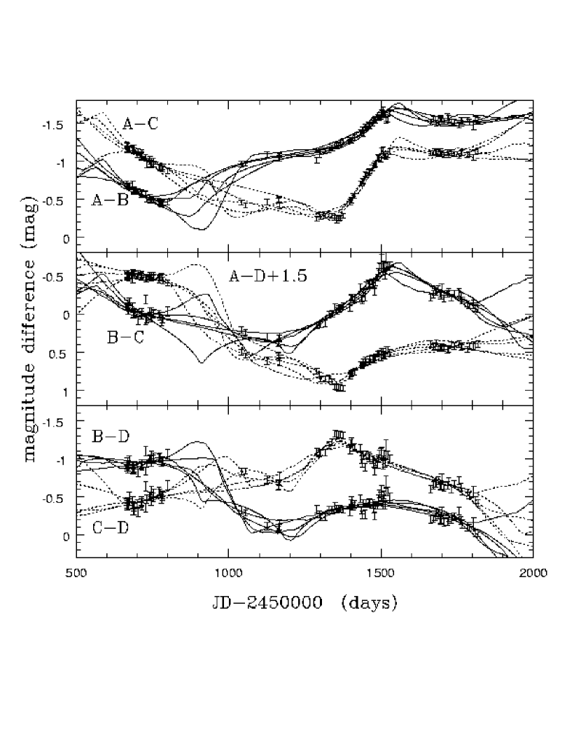
Figure 9: Difference light curves for the OGLE data and the 5 model light curves. The points show the 6 possible difference light curves ($m_{i}^{\alpha}-m_{i}^{\beta}$ with $\alpha\neq\beta$) that can be constructed from the OGLE data. The error bars are the OGLE uncertainties combined with a $\sigma_{0}=0.05$ mag systematic error in quadrature. The curves show the model light curve differences. The vertical scale of each panel is $2.0$ mag.

Figure 10: Difference light curves for the OGLE data and the 5 model light curves. We show the same light curves as in Fig. 9, but with the time scale expanded to show the behavior of the model light curves during the ten years before the start of the OGLE monitoring period. The vertical scale of each panel has been expanded to $5.0$ mag compared to the $2.0$ mag used in Fig. 9.

Figure 11: The reconstructed source fluxes for the light curves shown in Fig. 9. The lines connecting the points are only to guide the eye – the source flux can be estimated only where there is data. The shifts between the curves are another manifestation of how the monitoring period is not long enough for the light curves to determine the mean magnification (see §3.5 and Fig. 8). The points connected by the dashed lines show the mean source light curves found after averaging either the 5 source flux models shown here (“average5”) or these 5 plus the next 5 best models (“average10”). The mean magnitude of each source light curve was subtracted first, and the error bars show the dispersion of the light curves. The mean magnitude of these averaged light curves is arbitrary and was set simply to keep the light curves well-separated.

3.6 Examples of Light Curves

In this section we examine 5 of the 6 best light curve realizations found for the non-parametric models. We only save the light curves of the best model found for each set of physical parameters after varying all the variables for generating light curves (trajectory origin and velocity). The fourth best model had the same physical parameters as the third best, so its light curve was not preserved. All 5 cases have $\chi^{2}\simeq 200$ compared to $N_{dof}=290$, slightly over fitting the data given the additional $\sigma_{0}=0.05$ mag of systematic error we added to each data point (i.e. if we reduced $\sigma_{0}$ to $0.04$ mag we would find $\chi^{2}\simeq N_{dof}$). Three of the cases have $\log\hat{r}_{s}=15.75$, one has $\log\hat{r}_{s}=15.50$, and one has $\log\hat{r}_{s}=16.25$. All have $\kappa_{*}/\kappa=1$ and four out of five are thin disk models. The effective source velocities are $\hat{v}_{e}=14000$, $14600$, $29000$, $7100$ and $40000$ km/s respectively.

The goodness of fit of the non-parametric models is determined by how well the model light curves reproduce the six possible light curve differences (Eqn. 6). In Fig. 9 we show how well these 5 models fit the constraints. As expected from the $\chi^{2}$ values, the models reproduce the data with a general accuracy slightly exceeding the size of the error bars. In fact, even these models could be significantly improved by further local optimizations, because neither the effective velocity nor the source size is part of the local optimization process discussed in §2.2 (only the trajectory starting points and directions are optimized). In general, the light curves remain similar as they interpolate through the gaps in the data, although there is some divergence for the gap near 900 days. This is not true, however, if we extrapolate the behavior over longer time periods. Fig. 10 shows the light curves for the same models but with the time period expanded to cover the 10 years before the OGLE monitoring period. For typical models, the source crosses 1–3 Einstein radii in the OGLE data, so the light curves on longer time periods will show little correlation with those observed by OGLE. Since the OGLE data allows a wide range of magnitude offsets (§3.5, Fig. 8), most of the shifts in Fig. 10 are simply due to the difference between the mean magnification during the OGLE monitoring period and the global mean.

Fig. 11 shows the non-parametric estimates of the intrinsic source magnitude for the same model realizations. The offsets in the mean magnitudes are again due to the lack of convergence to the mean magnification. The rms of the intrinsic source variability ranges from $0.15$ mag to $0.29$ mag, considerably more than the level of $0.05$ mag we used in our parametric analysis. The scatter about a linear trend with time is smaller ($0.12$ to $0.14$ mag). This suggests that our parametric models were overly restrictive in their assumptions about the source variability, thereby forcing the microlensing variability to try to model some of the intrinsic variability. This may explain some of the velocity shifts between the analyses. The assumptions of the parametric model cannot, however, be completely unrealistic – for each image we do find light curve realizations where a constant source with an rms variability of $0.05$ mag is statistically consistent with the data. If such solutions exist for the individual images, then they also exist for all the images simultaneously. They must, however, occupy a small region of the allowed parameter space. The source flux variations of our five best solutions are quite similar (for example, all show a peak near day 1370), so in Fig. 11 we also show the statistical average of the source light curves for these solutions (scaled to the same mean magnitude) and the scatter of the light curves around the mean. Despite coming from models in wildly different regions of the magnification maps (see below), the scatter between the source light curves is considerably smaller than the overall variations. This continues to be true even if we construct the mean source fluctuations including the next set of 5 best realizations. Thus, it seems likely that the source quasar varied by approximately 0.5 mag during the monitoring period with a peak near day 1400.

INCLUDED ONLY AS JPEG FILE

Figure 12: Source trajectories superposed on magnification patterns for the best non-parametric realization ($\chi^{2}=186$ for $N_{dof}=290$). This is a mono-mass, thin disk model with $\log(\hat{r}_{s})=15.75$ and $\hat{v}_{e}=13900$ km/s. The gray scale shows the (unconvolved) magnification pattern for images A (top left), B (top right), C (lower left) and D (lower right). Darker colors indicate higher magnifications. The line shows the source trajectory across the pattern for the OGLE monitoring period. The large circle has a radius of $\langle\theta_{E}\rangle$ and the small circle has a radius of $\hat{r}_{s}$ (the smoothing scale). The circles are centered on the point corresponding to the initial epoch of the OGLE data. Depending on the background magnification, the source trajectory and the circles are either black or white.

INCLUDED ONLY AS JPEG FILE

Figure 13: Source trajectories superposed on magnification patterns for the second best non-parametric realization ($\chi^{2}=187$ for $N_{dof}=290$). This is a Salpeter, thin disk model with $\log(\hat{r}_{s})=15.75$ and $\hat{v}_{e}=14600$ km/s. See Fig. 12 for description.

INCLUDED ONLY AS JPEG FILE

Figure 14: Source trajectories superposed on magnification patterns for the third best non-parametric realization ($\chi^{2}=201$ for $N_{dof}=290$). This is a Salpeter, thin disk model with $\log(\hat{r}_{s})=15.75$ and $\hat{v}_{e}=29000$ km/s. See Fig. 12 for description.

INCLUDED ONLY AS JPEG FILE

Figure 15: Source trajectories superposed on magnification patterns for the fifth best non-parametric realization ($\chi^{2}=201$ for $N_{dof}=290$). This is a Salpeter, Gaussian disk model with $\log(\hat{r}_{s})=15.50$ and $\hat{v}_{e}=7100$ km/s. See Fig. 12 for description.

INCLUDED ONLY AS JPEG FILE

Figure 16: Source trajectories superposed on magnification patterns for the sixth best non-parametric realization ($\chi^{2}=201$ for $N_{dof}=290$). This is a Salpeter, thin disk model with $\log(\hat{r}_{s})=16.25$ and $\hat{v}_{e}=40200$ km/s. The trajectory for image B crossed the upper edge of the magnification pattern and then continued from the bottom edge, which is not shown. See Fig. 12 for description.

Finally, in Figs. 12–16 we show the source trajectories generating these light curves superposed on the magnification patterns. In order to make the caustics more easily visible, we did not convolve the patterns with the source structure of the realizations. The origin of the scatter in the magnitude offsets $\Delta\mu^{\alpha}$ (§3.5) and the offsets in average source brightness (Fig. 11) are easily understood from these figures. For example, image A was used as the magnitude reference point (because we measured $\Delta\mu^{\alpha}-\Delta\mu^{A}$), so the changes in the mean magnification of image A are responsible for the shifts in the average magnitude of the source (Fig. 11). In Figs. 13, 15 and 16 image A is produced in a magnified region, leading to fainter source magnitudes, while in Figs. 12 and 14 it a demagnified region, leading to a brighter source magnitude.

The magnification patterns are also useful for understanding the origins of the peaks in the light curves (Fig. 1). In particular, several studies (e.g. Yonehara Yonehara01 (2001), Shalyapin et al. Shalyapin02 (2002)) have attempted to model the peaks in the A and C light curves using simple fold caustic crossings or isolated point lenses to estimate the source structure. Sometimes models of the peak in the A light curve as a fold crossing is appropriate (e.g. Figs. 12 and 13). But in Figs. 14, 15 and 16 the peak is due to one or more caustic crossings associated with one or more cusps. The peaks seen in the light curve of image C are all associated with cusps, frequently arising from the high magnification regions outside the tip of the cusp (e.g. Fig. 14). Wyithe et al. (2000g ) drew a similar conclusion on more qualitative grounds. The light curve of image D can be smooth by staying inside the smooth part of a high magnification region (Fig. 12), using the finite source size to smooth out the variability of a region with very densely packed caustics (Figs. 13 and 15), staying in a smooth, demagnified region (Fig. 14) or by putting the caustic crossing inside the monitoring gaps (Fig. 16). The shear range of possibilities for producing quantitatively similar fits does not bode well for attempts to reconstruct source structures by making simplifying assumptions about the local caustic structures.

4 Discussion

The method we introduce in this paper reduces the problem of interpreting quasar microlensing data to a problem of computation rather than conceptualization. Any quasar microlensing data, from one or more lenses and both more or less complex, can be analyzed to derive physical results. We demonstrated the method using the most complex, single quasar microlensing data set, the OGLE light curves for the four images of Q2337+0305 to obtain simultaneous constraints on the microlens mass scale, source size, accretion disk structure, and the stellar mass fraction near the images. While all these issues have been studied in previous models of microlensing in Q2237+0305, this is the first time all the relevant physical properties of the system have been treated simultaneously.

We estimate that the effective source velocity is fairly high, $10200~{}\hbox{km/s}\mathrel{\raise 1.29167pt\hbox{$<$}\mkern-14.0mu\lower 2.58334pt\hbox{$\sim$}}v_{e}h\langle M/M_{\odot}\rangle^{-1/2}\mathrel{\raise 1.29167pt\hbox{$<$}\mkern-14.0mu\lower 2.58334pt\hbox{$\sim$}}39600$ km/s, which means that the source takes roughly 2 years to move one Einstein radius. Because the variability during the OGLE monitoring period was greater than during most of the preceding decade, the estimate of the effective velocity may be biased towards higher values than if we had modeled all the available data. We estimate statistically that the source is moving approximately $3300$ km/s from estimates for the peculiar velocity of the lens and the velocity dispersion of its constituent stars. Combining the probability distributions for the effective and physical source velocities, we obtain an estimate for the mean stellar mass of $\langle M\rangle\simeq 0.037h^{2}M_{\odot}$ ($0.0059h^{2}M_{\odot}\mathrel{\raise 1.29167pt\hbox{$<$}\mkern-14.0mu\lower 2.58334pt\hbox{$\sim$}}\langle M\rangle\mathrel{\raise 1.29167pt\hbox{$<$}\mkern-14.0mu\lower 2.58334pt\hbox{$\sim$}}0.20h^{2}M_{\odot}$) which is somewhat low. Unfortunately the mass estimate depends on the square of the velocities, so modest biases in the effective velocity from using the data during which the variability was largest or our approximate treatment of the internal motions of the stars make the systematic uncertainties in the mass estimate difficult to evaluate. Nevertheless, these mass estimates are consistent with previous results for this system (e.g. Lewis & Irwin Lewis96 (1996), Wyithe et al. 2000b ) and Galactic microlensing studies (e.g. Alcock et al. Alcock00 (2000)).

The lens galaxy in Q2237+0305 is composed of stars, with a lower bound of $\kappa_{*}/\kappa\mathrel{\raise 1.29167pt\hbox{$>$}\mkern-14.0mu\lower 2.58334pt\hbox{$\sim$}}0.5$ on the fraction of the surface mass density causing the flux variations. The limit rises to $\kappa_{*}/\kappa\mathrel{\raise 1.29167pt\hbox{$>$}\mkern-14.0mu\lower 2.58334pt\hbox{$\sim$}}0.7$ if we impose a prior of $0.2h^{2}M_{\odot}<\langle M\rangle<2h^{2}M_{\odot}$ on the masses of the microlenses, because models with low $\kappa_{*}$ require higher effective velocities (Einstein radii per year) corresponding to lower mass scales $\langle M\rangle$ in order to produce the same amount of variability. Since the lensed images in Q2237+0305 are passing through the bulge of a nearby spiral galaxy (Huchra et al. Huchra85 (1985)) we expect $\kappa_{*}\simeq\kappa$ for this system. However, our ability to estimate the stellar mass fraction for Q2237+0305 using microlensing data, indicates that we should also be able to estimate the stellar surface density fractions in other lenses where we expect dark matter to dominate the surface density with $\kappa_{*}/\kappa\sim 0.1$ to $0.2$ (see Schechter & Wambsganss Schechter02 (2002), Rusin, Kochanek & Keeton Rusin03 (2003)). While we kept the properties of the “macro” model (the total surface density and shear for each image) fixed in these calculations, these parameters could also be constrained by fits to the light curves. Our models with $\kappa_{*}/\kappa<1$ are closely related to models in which the mass distribution of the lens is more centrally concentrated than our standard isothermal model. This indicates that the microlensing data will favor the isothermal mass distribution over more centrally concentrated density profiles.

We find that the data is better fit by a standard thin accretion disk model than by a Gaussian model of the source’s surface brightness. We get an accurate estimate of the radius $r_{s}=2.6_{-1.2}^{+2.0}\times 10^{15}h^{-1}$ cm at which the disk temperature matches the wavelength of the observations ($2000\AA$ in the rest frame or $T_{s}\simeq 70000$ K). The results are consistent with black body emission and do not require non-thermal or optically thin emission processes. We estimate that the black hole mass is $M_{BH}\simeq 1.1_{-0.7}^{+1.4}\times 10^{9}h^{-3/2}\eta_{0.1}^{1/2}(L/L_{E})^{-1/2}M_{\odot}$, which means that $r_{s}$ corresponds to approximately 8 Schwarzschild radii from the black hole. While reassuringly consistent, our treatment of the source structure has limitations. First, the physical model for the accretion disk is more appropriate for the outer regions of a thin disk than for the inner regions. Second, we assumed that the disk was viewed face-on and was circular. A more realistic model would need to use an inclined disk.

The only practical limitation to our approach is its computational intensity. Our present analysis considered 208 different combinations of stellar density, stellar mass function, source structure and source size, generating 40 billion non-parametric light curve realizations, and required approximately 2 processor-months to do the final calculations. The problem is, however, trivially parallel, making larger parameter surveys relatively easy to conduct simply by using more computers (it would take one day given 60 processors). Improvements in the sampling of the variables or the strategies for rapidly discarding poor light curve trials should significantly reduce the number of trials needed to achieve the same statistical results. For example, we uniformly sampled the $\log\hat{r}_{s}$/$\log\hat{v}_{e}$ plane, but only a restricted region of the plane produces statistically acceptable solutions (see Fig. 4). One major systematic limitation to our estimate of the mass scale $\langle M\rangle$ is our inability to correctly treat the internal motions of the stars in the lens galaxy using static magnification patterns. Adding the internal motions requires tracing the source trajectories through a sequence of magnification patterns (e.g. Wambsganss & Kundic Wambsganss95 (1995)). This adds little to the execution time, but requires large amounts of memory. Models of the OGLE light curves of Q2237+0305 including the stellar motions require 200-400 time steps (resolving the mean stellar motion in steps of $0.01$-$0.02\langle\theta_{E}\rangle$) for each image, all 13-26 Gbytes of which must be stored in memory. Fortunately, most multi-processor computers which would significantly speed the completion of the calculations also have the memory needed to hold such large data spaces.

At present, only Q2237+0305 has light curve data that justifies such computational intensity simply due to the lack of monitoring data for most lenses. The Einstein crossing time due to lens motions scales as $(1+z_{l})(D_{OL}D_{LS}/D_{OS})^{1/2}$, which means that systems with low lens redshifts like Q2237+0305 have shorter time scales for microlensing variability (Kayser & Refsdal Kayser89 (1989)). But they are not enormously shorter – the other quasar lenses with known redshifts have time scales that are only 2–3 times longer. Even if the variability rates of the roughly 30 available quasar lenses are three times slower than in Q2237+0305, monitoring all of them routinely generates data equivalent to 3 OGLE light curves each year. These data can be significantly enhanced by systematically measuring the differences between the continuum and emission line flux ratios of the images (e.g. Lewis et al. Lewis98 (1998), also radio, Falco et al. Falco96 (1996) or mid-infrared Agol, Jones & Blaes Agol00 (2000), Wyithe, Agol & Fluke 2002a ). Since the emission lines are generated on scales significantly larger than the continuum, the differences in the flux ratios provide immediate constraints on the location of the images in the magnification pattern and on the relative sizes of the two emitting regions. A final, but important, advantage of monitoring as many lenses as possible is that they are statistically independent. Each new image in a new lens lies in a random region of a new magnification pattern, providing new constraints without the long term temporal correlations of data obtained by monitoring a particular lens. Moreover, estimates of the stellar mass scale $\langle M\rangle$ in any particular lens are ultimately limited by the uncertain peculiar velocity of the lens. Only by combining the estimates from multiple lenses can we ever obtain an accurate estimate.

Appendix A Generating Periodic Magnification Maps

We use the ray-shooting method (e.g. Schneider et al. Schneider92 (1992)) to compute the source plane magnification patterns. We use a particle-particle/particle-mesh (P³M, Hockney & Eastwood Hockney81 (1981)) algorithm to separate the long and short range effects of the stars. The source plane region is a square with outer dimension $L_{u}$, pixel scale $\Delta u$ and a dimension $N_{u}=L_{u}/\Delta u$ that is chosen to be a power of 2. The image plane is an $L_{x}\times L_{y}$ rectangle defined by $L_{x}|1-\kappa-\gamma|=L_{y}|1-\kappa+\gamma|=L_{u}$. The image plane pixel scale is $\Delta x$, so image plane dimensions of $N_{x}=L_{x}/\Delta x$ and $N_{y}=L_{y}/\Delta x$ differ. We choose the larger dimension of the image plane to be a power of 2. The smaller dimension of the image plane is determined by the axis ratio of the rectangle. In order to have both square pixels and an exact periodicity of both the source and image planes, the integer array dimensions must satisfy $N_{x}|1-\kappa-\gamma|=N_{y}|1-\kappa+\gamma|$. We impose the constraint by first finding the smaller dimension which comes closest to satisfying it given the fixed larger dimension and then making a small adjustment to the shear value ($\Delta\gamma\simeq N_{y}^{-1}\simeq 0.001$) so that it becomes exact. These adjustments are so small that they have no physical consequences for our results.

The long-range effects of the stars are computed using Fourier methods. The mass of each star is assigned to the nearest grid points using weights determined by the distance of the star from the pixels (the TSC, triangle-shaped cloud). We then compute the deflections produced by the stars by convolving the surface density with the deflection kernels ${\bf\alpha_{s}}$. We completely separate the long and short range effects of the gravity using spline models for the surface density. We use the spline density distribution which is

$$\kappa_{s}(R,s)={2\over\pi s^{2}}\left(1-{r^{2}\over s^{2}}\right)$$ (A1)

for $R<s$ and equal to zero for $R>s$. For the convolution we use the deflection pattern of the surface density distribution, $\kappa_{s}(R,s)-\kappa_{s}(R,a)$, which has zero net mass. The inner scale $s=5\Delta x$ sets the boundary between the the long range and short range effects of the star. The outer scale, $a=\hbox{min}(L_{x},L_{y})/2$, guarantees that $\kappa$ is the total surface density. It does, however, limit the long range stochasticity of the potential because fluctuations in the stellar density on scales larger than $a$ are filtered out of the gravitational field. An attentive reader will have noticed that the smaller dimension of the image plane is not generally a power of 2. We use the FFTW (“Fastest Fourier Transform in the West,” Frigo & Johnson Frigo98 (1998)) Fourier transform package, which is both fast and handles such transforms without any special treatment. This gives the long range deflection field ${\bf\alpha_{g}}$. On scales smaller than the inner scale, $s=5\Delta x$, the deflection field computed from the convolution must be corrected from that of the spline to that of a real point mass. Each image plane pixel is associated with a list of all stars within $s$ of the pixel boundaries. When we compute ray deflections for that pixel we add the true deflection from each of these stars minus the contribution from the spline density that we included in the long range deflection field ${\bf\alpha_{g}}$ to give the particle contribution to the deflection ${\bf\alpha_{p}}({\bf x})$.

The total deflection is

$${\bf u}={\bf x}\left(\begin{array}[]{cc}1-\kappa-\gamma&0\\ 0&1-\kappa+\gamma\end{array}\right)-{\bf\alpha_{g}}({\bf x})-{\bf\alpha_{p}}({\bf x}).$$ (A2)

The terms hide two cancellations. The outer, negative spline density in the gridded deflection, ${\bf\alpha_{g}}$, is needed to allow the $\kappa$ in the deflections to be the total surface density $\kappa$ rather than $\kappa_{s}=\kappa-\kappa_{*}$. This could be changed without any particular problem. The inner spline region ($R<s$) for each star is added in ${\bf\alpha_{g}}$ and then subtracted in ${\bf\alpha_{p}}$ so that the final deflections exactly match that of a point mass. Note that a similar scheme would work equally well for models of substructure. Because the deflections of the stars are exactly periodic on both the image and source planes, a single pass over the image plane can identify all rays which will be mapped onto the source plane and source trajectories can be continuously traced across the source plane boundaries. Similarly if we allow the microlenses to move, their trajectories are periodic on the lens plane grid. We set all scales using the average Einstein radius of the stars $\langle\theta_{E}\rangle$. Typically we generated a magnification pattern with $L_{u}=40\langle\theta_{E}\rangle$ and $N_{u}=2048$ with source plane pixels $\Delta u\simeq 0.02\langle\theta_{E}\rangle$. We traced rays on a uniform grid with a minimum image plane resolution of $0.01\langle\theta_{E}\rangle$ and required an average of $100$ rays per source pixel.

Although the magnification patterns for a fixed mass function would appear to depend on three variables (the smooth surface density $\kappa$, the stellar surface density $\kappa_{*}$, and the shear $\gamma$), the mass sheet degeneracy (Paczynski Paczynski86 (1986) for the case of microlensing) means that there are only two independent variables. Here we derive a generalized version of the mass sheet degeneracy. Consider two systems, labeled A and B, defined by point masses with Einstein radii $b_{i}$ at positions ${\bf x}_{i}$ in an external shear $\gamma$, a smooth convergence $\kappa_{s}$, and a mean convergence due to the stars of $\kappa_{*}$. The shear and convergence define a reduced shear $g=\gamma/(1-\kappa_{s})$. The x-component of the lens equations for the two systems are

$$u_{A}=(1-\kappa_{sA})(1-g_{A})x_{A}-\sum_{i}b_{A,i}^{2}{x_{A}-x_{A,i}\over\left|{\bf x}_{A}-{\bf x}_{A,i}\right|^{2}}$$ (A3)

and

$$u_{B}=(1-\kappa_{sB})(1-g_{B})x_{B}-\sum_{i}b_{B,i}^{2}{x_{B}-x_{B,i}\over\left|{\bf x}_{B}-{\bf x}_{B,i}\right|^{2}}$$ (A4)

respectively. Now assume that the two equations can be related by simultaneously rescaling the source plane coordinates, ${\bf u}_{B}=\alpha{\bf u}_{A}$, the lens plane coordinates, ${\bf x}_{B}=\beta{\bf x}_{A}$, and the Einstein radii, $b^{2}_{B,i}=\xi b^{2}_{B,i}$. For the lens equations this leads to the constraints that the two systems must have the same reduced shear, $g_{A}=g_{B}$, that the convergences are related by $1-\kappa_{sA}=(1-\kappa_{sB})\beta/\alpha$, and that the Einstein radii are related to the coordinate rescalings by $\xi=\alpha\beta$. The same scalings hold for the magnifications, with $\mu_{B}=\beta^{2}\mu_{A}/\xi=\beta\mu_{A}/\alpha$. The average surface density of the stars transforms as $\kappa_{*B}=\kappa_{*A}\xi/\beta^{2}$ and the source plane velocity scales as $v_{e,B}=\alpha v_{e,A}$. The familiar mass sheet degeneracy is found by holding the lens plane scale fixed ($\beta\equiv 1$) and setting $\kappa_{sA}=0$, in which case $\xi=\alpha=1-\kappa_{sB}$, $b_{B}^{2}=(1-\kappa_{sB})b_{A}^{2}$, and $\kappa_{*B}=|1-\kappa_{sB}|\kappa_{*A}$. While there is no new physics in this generalization, it can be computationally useful.

References

- (1) Afonso, C., Alard, C., Albert, J.N., et al., 2000, ApJ, 532, 340
- (2) Agol, E., Jones, B. & Blaes, O., 2000, ApJ, 545, 657
- (3) Alard, C., 2000, A&AS, 144, 363
- (4) Alcalde, D., Mediaville, E., Moreau, O., et al., 2002, ApJ, 572, 729
- (5) Alcock, C., Allsman, R.A., Alves, D.R., et al., 2000, ApJ, 541, 734
- (6) Chang, K., & Refsdal, S., 1979, Nature, 282, 561
- (7) Corrigan, R.T., Irwin, M.J., Arnaud, J., et al., 1991, AJ, 102, 34
- (8) Crotts, A., 1992, ApJL, 399, L43
- (9) Di Stefano, R.R. & Esin, A.A., 1995, ApJL, 448, L1
- (10) Eisenstein, D.J., & Hu, W., 1999, ApJ, 511, 5
- (11) Falco, E.E., Lehar, J., Perley, R.A., Wambsganss, J., & Gorenstein, M.V., 1996, Aj, 112, 897
- (12) Falco, E.E., Impey, C.D., Kochanek, C.S., Lehar, J., McLeod, B.A., Rix, H.-W., Keeton, C.R., Munoz, J.A., & Peng, C.Y., 1999, ApJ, 523, 617
- (13) Foltz, C.B,. Hewitt, P.C., Webster, R.L., Lewis, G.F., 1992, ApJL, 386, L43
- (14) Frigo, M., & Johnson, S.G., 1998, proceedings of the IEEE International Conference on Acoustics, Speech and Signal Processing, volume 3, 1381
- (15) Gould, A., 1992, ApJ, 392, 442
- (16) Grieger, B., Kayser, S., & Refsdal, S., 1986, Nature, 324, 126
- (17) Hockney, R. W. and Eastwood, J. W. 1981, Computer Simulation Using Particles, (McGraw-Hill: New York)
- (18) Huchra, J., Gorenstein, M., Kent, S., Shapiro, I., Smith, G., Horine, E., & Perley, R., 1985, AJ, 90, 691
- (19) Kayser, R., Refsdal, S., & Stabell, R., 1986, A&A, 166, 36
- (20) Kayser, R., & Refsdal, S., 1989, Nature, 338, 745
- (21) Kochanek, C.S., Kolatt, T.S., & Bartelmann, M., 1996, ApJ, 473, 610
- (22) Kochanek, C.S., 2002, ApJ, 578, 25
- (23) Kochanek, C.S., & Dalal, N., 2003, ApJ submitted [astro-ph/0302036]
- (24) Kogut, A., et al., 1993, ApJ, 419, 1
- (25) Kundic, T., & Wambsganss, J., 1993, ApJ, 404, 455
- (26) Lehar, J., Falco, E.E., Kochanek, C.S., McLeod, B.A., Impey, C.D., Rix, H.-W., Keeton, C.R., & Peng, C.Y., 2000, ApJ, 536, 584
- (27) Lewis, G.F., & Irwin, J.J., 1995, MNRAS, 276, 103
- (28) Lewis, G.F., & Irwin, J.J., 1996, MNRAS, 283, 79
- (29) Lewis, G.F., Irwin, M.J., Hewitt, P.C., & Foltz, C.B., 1998, MNRAS, 295, 573
- (30) Lewis, G.F., & Ibata, R.A., 2003, MNRAS, 340, 562
- (31) Mao, S., & Paczynski, B., 1991, ApJL, 374, L37
- (32) Mao, S., 2001, in Gravitational Lensing: Recent Progress & Future Goals (ASP #237), eds. T.G. Brainerd & C.S. Kochanek (ASP: San Francisco) 215
- (33) Ostensen, R., Refsdal, S., Stabell, R., et al., 1996, A&A, 309, 590
- (34) Paczynski, B., 1986, ApJ, 301, 503
- (35) Paczynski, B., 1996, ARA&A, 34, 419
- (36) Racine, R., 1992, ApJL, 395, 65L
- (37) Rauch, K.P., & Blandford, R.D., 1991, ApJL, 381, 39L
- (38) Refsdal, S., & Stabell, R., 1993, A&A, 278, 5L
- (39) Rusin, D., Kochanek, C.S., & Keeton, C.R., 2003, ApJ in press [astro-ph/0306096]
- (40) Saust, A.B., 1994, A&AS, 103, 33
- (41) Schechter, P. L., & Wambsganss, J. 2002, ApJ, 580, 685
- (42) Schneider, P., & Weiss, A. 1887, A&A, 171, 49
- (43) Schneider, P., Ehlers, J., & Falco, E.E., 1992, Gravitational Lenses, (Springer Verlag: Berlin)
- (44) Schramm, T., Kayser, R., Chang, K., Nieser, L., & Refsdal, S., 1993, A&A, 268, 350
- (45) Seitz, C., & Schneider, P., 1994, A&A, 288, 1
- (46) Seitz, C., Wambsganss, J., & Schneider, P., 1994, A&A, 288, 19
- (47) Shalyapin, V.N., Goicoechea, L.J., Alcade, D., Mediavilla, E., Munoz, J.A., & Gil-Merino, R., 2002, ApJ, 579, 127
- (48) Shapiro, S.L. & Teukolsky, S.A., 1983, Black Holes, White Dwarfs & Neutron Stars, (Wiley: New York)
- (49) Wambsganss, J., Paczynski, B., & Schneider, P., 1990, ApJL, 358, 33L
- (50) Wambsganss, J., & Kundic, T., 1995, ApJ, 450, 19
- (51) Wambsganss, J., 2001, in Gravitational Lensing: Recent Progress & Future Goals (ASP #237), eds. T.G. Brainerd & C.S. Kochanek (ASP: San Francisco) 185
- (52) Webster, R.L., Ferguson, A.M.N., Corrigan, R.T., & Irwin, M.J., 1991, AJ, 102, 1939
- (53) Witt, H.J., Kayser, R., & Refsdal, S., 1993, A&A, 268, 501
- (54) Witt, H.J., & Mao, S., 1994, ApJ, 429, 66
- (55) Witt, H.J., & Mao, S., 1994, ApJ, 430, 505
- (56) Wozniak, P.R., Alard, C., Udalski, A., Szymanski, M., Kubiak, M., Pietrzynski, G., & Zebrun, K., 2000, ApJL, 529, 88
- (57) Wozniak, P.R., Udalski, A., Szymanski, M., Kubiak, M., Pietrzynski, G., Soszynski, I., & Zebrun, K., 2000, ApJL, 540, 65
- (58) Wyithe, J.S.B., Webster, R.L., & Turner, E.L., 1999, MNRAS, 309, 261
- (59) Wyithe, J.S.B., Webster, R.L., & Turner, E.L., 2000a, MNRAS, 312, 843
- (60) Wyithe, J.S.B., Webster, R.L., & Turner, E.L., 2000b, MNRAS, 315, 51
- (61) Wyithe, J.S.B., Webster, R.L., Turner, E.L., & Mortlock, D.J., 2000c, MNRAS, 315, 62
- (62) Wyithe, J.S.B., Webster, R.L., & Turner, E.L., 2000d, MNRAS, 315, 337
- (63) Wyithe, J.S.B., Webster, R.L., & Turner, E.L., 2000e, MNRAS, 318, 762
- (64) Wyithe, J.S.B., Webster, R.L., Turner, E.L. & Agol, E., 2000f, MNRAS, 318, 1105
- (65) Wyithe, J.S.B., Webster, R.L., & Turner, E.L., 2000g, MNRAS, 318, 1120
- (66) Wyithe, J.S.B., & Turner, E.L., 2001, MNRAS, 320, 21
- (67) Wyithe, J.S.B., Agol, E., & Fluke, C.J., 2002, MNRAS, 331, 1041
- (68) Wyithe, J.S.B., Agol, E., Turner, E.L., & Schmidt, R.W., 2002, MNRAS, 330, 575
- (69) Yonehara, A., 2001, ApJ, 548, 127