Physical Evidence for Dark Energy

Abstract

We present measurements of the angular cross-correlation between luminous red galaxies from the Sloan Digital Sky Survey and the cosmic microwave background temperature maps from the Wilkinson Microwave Anisotropy Probe. We find a statistically significant achromatic positive correlation between these two data sets, which is consistent with the expected signal from the late Integrated Sachs-Wolfe (ISW) effect. We do not detect any anti-correlation on small angular scales as would be produced from a large Sunyaev-Zel’dovich (SZ) effect, although we do see evidence for some SZ effect for our highest redshift samples. Assuming a flat universe, our preliminary detection of the ISW effect provides independent physical evidence for the existence of dark energy.

I Introduction

As photons from the Cosmic Microwave Background (CMB) travel to us from the surface of last scattering, they can experience a number of physical processes. These include the Sunyaev-Zel’dovich (SZ(Zel’dovich & Sunyaev, 1967)) effect, which is the inverse Compton scattering of CMB photons by a hot ($T>10^{7}$ K) ionized gas(Birkinshaw, 1999), and the late Integrated Sachs–Wolfe (ISW(Sachs & Wolfe, 1967; Hu & Dodelson, 2002)) effect, which is the integrated differential gravitational redshift caused by the evolution of gravitational potentials along the path traveled by the photons. At frequencies less than $217$ GHz, the SZ effect produces an anti-correlation between the temperature of the CMB and galaxies on small angular scales. The ISW effect generates a weak positive correlation at large angular scales for all frequencies(Peiris & Spergel, 2000). For a universe with a flat geometry(Spergel et al., 2003), the detection of any ISW effect provides strong physical evidence for the existence of dark energy, and can be used to measure its equation of state (Coble, Dodelson, & Frieman, 1997; Caldwell98, ; Hu, Seljak, White, & Zaldarriaga, 1998; Corasaniti et al., 2003). In this paper, we attempt the detection of the ISW and SZ effects through the cross-correlation of new, large area, clean galaxy and CMB maps of the sky (Peiris & Spergel, 2000; Cooray, 2002), which reduce the errors due to sample variance on large scales and the Poisson error on small scales relative to that of previous attempts(Boughn & Crittenden, 2003; Fosalba & Gaztañaga, 2003; Myers2003, ; Nolta et al., 2003).

II Data & Estimators

The parent SDSS galaxy data used herein is nearly 25 million galaxies taken from $\simeq 3400$ square degrees of the sky imaged by the Sloan Digital Sky Survey (SDSS(Fukugita1996, ; Gunn1998, ; York et al., 2000; Abazajian2003, ; Hogg2001, ; Pier2003, ; Smith2002, ; Stoughton2002, )). We apply a flux limit of $i<21$ and regions with poor image quality have been excluded from our analysis (i.e., data with a point–spread function of worse than 1.5 arcseconds). From this basic data set, we have constructed four different subsets of galaxies using both the Luminous Red Galaxy (LRG) selection method(Eisenstein et al., 2001) and a photometric redshift estimate for every galaxy(Budavári et al., 2000). As shown in Figure 1, these subsamples span a range of redshift from $z\sim 0.3$ to $z\sim 0.8$, providing an efficient method for tracing the large–scale distribution of galaxies in the Universe as a function of redshift.

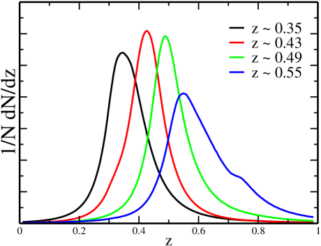
Figure 1: The photometric redshift distributions for the four LRG subsamples, taking into account the covariance between photometric redshift and galaxy type. To select these galaxies, we imposed a color cut of $0.7(g-r)+1.2((r-i)-0.18)>1.6$ and $(g-r)>1$. We then define $d_{\perp}=(r-i)-(g-r)/8$, and step through $d_{\perp}$ in increments of 0.2 starting at $0.2<d_{\perp}<0.4$ and ending at $d_{\perp}>0.8$ to determine our four redshift samples, from lowest to highest redshift respectively. There are 0.4 million LRGs in the $z\sim 0.35$ subsample, 0.8 million in the $z\sim 0.43$ subsample, 1 million in the $z\sim 0.49$ subsample, and 0.7 million in the $z\sim 0.55$ subsample.

For the CMB data, we use the 3 primary combined-channel maps (Q, V, W) from the Wilkinson Microwave Anisotropy Probe (WMAP(Spergel et al., 2003)), and the “clean” map of Tegmark et al.(Tegmark et al., 2003). We also apply a mask to exclude foreground contamination from the Galaxy (kp12 for the V & W bands and kp2 for the Q band). To isolate the ISW effect, we also generate a smoothed version of the “clean” map, by applying a Gaussian kernel with a FWHM of one degree to remove CMB primary anisotropies on small angles.

The natural pixelization scheme for the WMAP maps is HEALPix while for the galaxies it is SDSSPix. The latter is a new, hierarchical equal-area pixelization scheme developed specifically for the SDSS geometry and fast correlation statistics. For our primary calculations we use the higher resolution SDSSPix for accurate weighting, while for the extensive Monte Carlo simulations discussed below, we use HEALPix to take advantage of the SpICE(Szapudi, Prunet, & Colombi, 2001) for fast cross–correlation estimations. Both methods required re–pixelization of the original maps. We have tested our re-pixelization methods by comparing the auto-correlation functions of the original and re–sampled maps and we find identical results and errors.

For the cross-correlation measurement, we use a simple pixel-based estimator. For each pixel $i$ in our map, we determine the galaxy and temperature over-densities ($\Delta^{\rm g}$ & $\Delta^{\rm T}$, respectively),

$$\Delta^{\rm g}_{i}=\frac{n^{\rm g}_{i}-\overline{n^{\rm g}}}{\overline{n^{\rm g}}_{i}},\qquad\Delta^{\rm T}_{i}=T_{i}-\overline{T},$$ (1)

where $T_{i}$ is the temperature in pixel $i$, $\overline{T}$ is the mean temperature, $n^{\rm g}_{i}$ is the total number of galaxies in pixel $i$, and $\overline{n^{\rm g}}_{i}$ is expected number of galaxies in pixel $i$. In addition, we can optimally weight each pair of pixels to account for the variation of signal-to-noise (S/N) in the pixels. Therefore, the two–point cross-correlation function at angular separation $\theta_{\alpha}$ is given by

$$w_{\rm gT}(\theta_{\alpha})=\frac{\sum_{i,j}\Delta^{\rm g}_{i}\,\Delta^{\rm T}_{j}\,f_{i}\,s_{j}\,\Theta^{\alpha}_{ij}}{\sum_{n,m}f_{n}s_{m}\Theta^{\alpha}_{n,m}}\ ,$$ (2)

where $\theta_{\alpha}$ is the central value of an angular correlation bin, $f_{i}$ is the fraction of pixel $i$ unmasked, $s_{i}$ is the inverse of the noise in the WMAP pixel, and $\Theta^{\alpha}_{ij}$ is unity if the separation between the pixels is within this angular bin and zero otherwise. On large angular scales the optimal CMB weighting is uniform (i.e., $s_{i}=1$, except where masked) as the signal is dominated by sample variance rather than Poisson noise. For completeness, we calculate the cross-correlation functions for both the uniform and noise–weighted schemes.

To estimate the covariance $C(\theta_{\alpha},\theta_{\beta})$, we use two methods: jack–knife errors and random CMB maps. For the former, we divide our total area into $N_{J}$ equal-area subsamples and use the jack–knife estimator(Scranton et al., 2002),

$$C_{J}(\theta_{\alpha},\theta_{\beta}) = \frac{N_{J}-1}{N_{J}}\sum^{N_{J}}_{i=1}(\overline{w_{\rm gT}}(\theta_{\alpha})-w_{\rm gT,i}(\theta_{\alpha}))$$ (4)

$$\times(\overline{w_{\rm gT}}(\theta_{\beta})-w_{\rm gT,i}(\theta_{\beta})),$$

where $\overline{w_{\rm gT}}(\theta)$ is the mean of $w_{\rm gT}(\theta)$ for the $N_{J}$ measurements and $w_{{\rm gT},i}(\theta)$ is the measurement of the cross-correlation excluding the $i$th subsample. In order to produce a stable estimation of the covariance matrix (non-singular and positive definite), we set $N_{J}=2N_{\theta}$, where $N_{\theta}$ is the number of angular bins. Tests with different values of $N_{J}$ near to $2N_{\theta}$ generally produced values of $\chi^{2}$ (see Section IV.2) within 15% of the values obtained using $N_{J}=2N_{\theta}$.

While the jack–knife method gives a good approximation of the sample variance, it is less sensitive to variance on angular scales larger than the survey size. For a more conservative estimate of the covariance, we generated 200 random CMB maps based on the angular power spectrum of the “clean” map and 200 random CMB maps based on the angular power spectrum of our smoothed WMAP map. These maps were cross-correlated against the four galaxy maps (using SpICE(Szapudi, Prunet, & Colombi, 2001)) and the results were re-sampled into the same angular bins as used in the SDSSPix analysis. The covariance matrix is then

$$C_{R}(\theta_{\alpha},\theta_{\beta}) = \frac{1}{N}\sum^{N=200}_{i=1}(\overline{w_{\rm gT}}(\theta_{\alpha})-w_{\rm gT,i}(\theta_{\alpha}))$$ (6)

$$\times(\overline{w_{\rm gT}}(\theta_{\beta})-w_{\rm gT,i}(\theta_{\beta})).$$

III Results

We present the cross–correlation functions for the four redshift subsamples and the four WMAP maps in Figure 2. For the three highest redshift galaxy subsamples, we find a consistent non–zero signal. We also find that the cross–correlation signal is achromatic in the Q, V, W frequency maps. We see little evidence for an anti-correlation between the galaxy density and CMB temperature on the smallest angular scales, as expected from the SZ effect. For the lowest redshift subsample, we see a different shape to the cross–correlation function and all the angular bins are consistent with zero within their errors. This lowest redshift subsample also shows a lack of agreement between the Q, V, and W frequency maps.

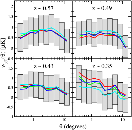
Figure 2: The uniform-weighted galaxy–WMAP cross-correlation functions for the four galaxy subsamples. The shaded boxes show the measurement and the $1\sigma$ jack–knife errors for the “clean” galaxy–WMAP cross-correlation function. The errors on the other functions are nearly identical. The Q map is given by the red line, V by the green line, W by the blue line and smoothed map by the cyan line.

IV Discussion

IV.1 Systematic Error Tests

Our primary concern is the possible contamination of the CMB signal by residual Galactic synchrotron or dust emission and the galaxy catalogs by Galactic stars. This could result in a non–zero correlation between the maps. To check against this, we calculate the stellar over-density in each pixel, using the same color cuts as for the four galaxy subsamples discussed above, and substitute these over-densities into Equation 2. For the three highest redshift subsamples, we find flat, featureless star-WMAP cross-correlation functions consistent with zero at the $1\sigma$ level. For the lowest redshift sample ($z\sim 0.35$), the star-WMAP cross-correlation function is nearly identical to the galaxy–WMAP measurement, suggesting significant contamination.

The cross–correlation functions for the three highest redshift galaxy subsamples are achromatic in the WMAP Q, V and W frequency maps. In addition to the visual agreement in Figure 2, we cross-correlated the three highest redshift galaxy subsamples against four linear combinations of the Q, V, and W maps. These combination were designed to detect achromatic effects (${\rm Q-V}$ and ${\rm V-W}$) and possible contamination from synchrotron (${\rm(9Q-12V+3W)/16}$) and dust emission (${\rm(3Q-12V+9W)/16}$). In all 12 cross-correlation functions, the signal was suppressed relative to our original galaxy–WMAP signal by a factor of $\sim\!10$ on all angular scales with errors consistent with Poisson noise from the galaxies. Likewise, the shapes of the cross-correlation functions were dissimilar to those seen for the galaxy–WMAP cross-correlation functions. These observations confirm that our galaxy–WMAP measurements are not due to contamination by synchrotron or dust emission from the Galaxy, or synchrotron emission the host galaxies themselves(Myers2003, ), i.e., over the frequency range probed by WMAP, the intensity of any synchrotron emission should decrease by an order of magnitude from Q to W.

IV.2 Significance Tests

As with any angular correlation measurement, the individual angular bins are highly correlated. Therefore, we need to consider the the full covariance matrix ($C_{R,J}$) when checking the statistical significance of our measurements against the null hypothesis of a zero cross–correlation function. Our $\chi^{2}$ values are given by

$$\chi_{R,J}^{2}=w_{\rm gT}C_{R,J}^{-1}w_{\rm gT},$$ (7)

where $C_{R,J}$ is the covariance matrix derived from either Eqn 6 (random maps) or Eqn 4 (jack–knife errors) respectively. The $\chi^{2}$ values for each of our uniform weighted cross–correlation functions, including the smoothed map, are given in Table 1 using both covariance matrices. These values are in reasonable agreement with other measurements of similar cross-correlation functions at larger angles (Boughn & Crittenden, 2003; Nolta et al., 2003). The choice of weighting for the CMB pixels does not change our results significantly.

For the three highest redshift samples, we exclude the null hypothesis at $\geq 90\%$ confidence for every WMAP band and the “clean” and smoothed maps using the jack–knife errors. For the random map errors, we can exclude the null hypothesis at $\geq 90\%$ for only the two highest redshift samples (excluding the Q band and smoothed map). Excluding angular bins on scales $<2$ degrees increases the significance of the smoothed detection with the random map errors but not to the 90% confidence threshold. Checking the number of random maps with $\chi^{2}$ greater than the values in Table 1 verifies that our confidence estimates are correct.

Table 1: The $\chi^{2}$ values derived from both covariance matrices (jack–knife errors given in parentheses) for $N_{\theta}=10$ angular bins

Subsample	Q	V	W
$z\sim 0.55$	10.4 (16.3)	18.6 (20.4)	35.7 (25.3)
$z\sim 0.49$	19.9 (28.3)	21.6 (32.0)	19.9 (17.0)
$z\sim 0.43$	8.4 (16.3)	5.9 (19.5)	13.0 (37.2)
$z\sim 0.35$	33.9 (14.6)	54.2 (24.6)	27.3 (33.3)
Subsample	“Clean”	Smoothed
$z\sim 0.55$	15.8 (27.1)	7.0 (20.8)
$z\sim 0.49$	17.0 (30.2)	11.0 (24.8)
$z\sim 0.43$	6.8 (34.1)	5.6 (30.1)
$z\sim 0.35$	32.5 (27.3)	12.8 (11.2)

We complement the $\chi^{2}$ statistical analysis by applying the False Discovery Rate (FDR (Miller2001, ; Hopkins2002, )) technique to the combination of all of our cross–correlation functions into a single significance test of our whole signal. The utility of the FDR statistic over combining the individual $\chi^{2}$’s for different redshift slices comes from the fact that it is conservative and designed to work with highly correlated datasets. FDR works by controlling $\alpha$, the fraction of false detections compared to the total number of detections(Miller2001, ). For a given $\alpha$, the FDR technique provides a threshold above which bins are rejected from a null hypothesis, in this case $w_{gT,i}=0$ for all $i$ angular bins, with the guarantee that the true number of errors is always $\leq\alpha$. Using the three highest redshift subsamples, cross-correlated with the five CMB maps ($5\times 10\times 3=150$ bins in total), we reject, with an $\alpha=0.25$, 144 bins with the jack–knife errors and 113 bins for the random CMB map errors. Therefore, at least 108 (84) of our 150 angular bins are rejected from the null hypothesis using the jack–knife (random maps) errors.

V Theoretical Models

We now compare our results to simple physical models of the ISW and SZ effects. A more detailed theoretical analysis of our results will appear in a future paper. We assume here a $\Lambda$CDM cosmology given by the fits to the WMAPext data(Spergel et al., 2003): $\Omega_{\rm tot}=1$, $h=0.72$, $\Omega_{\rm m}=0.29$, $\Omega_{\rm b}=0.047$, $\sigma_{8}=0.9$, and $n_{\rm s}=0.99$.

We expect our observed cross-correlation functions to be the sum of the induced correlations from the ISW and SZ effects(Peiris & Spergel, 2000), i.e.,

$$w_{\rm gT}(\theta)=w_{\rm ISW}(\theta)+w_{\rm SZ}(\theta).$$ (8)

The ISW effect is generated by the decay of gravitational potentials in an open or dark energy dominated universe. This decay couples to the dark matter momentum, meaning that our galaxy-temperature cross-correlations will be a function of the galaxy-momentum power spectrum:

$$w_{\rm ISW}(\theta)=\bar{b}\int\frac{dk}{k}\int d\chi\,{\cal K}_{\rm ISW}(k,\theta,\chi)\,D(\chi)\,P(k),$$ (9)

where $\chi$ is the co-moving distance, $D(\chi)$ is the linear growth factor, $P(k)$ is the linear dark matter power spectra and $\bar{b}$ is the linear galaxy bias at the peak of the galaxy redshift distribution ($\bar{z}$). The kernel (${\cal K}_{\rm ISW}$) is given by

$${\cal K}_{\rm ISW}(k,\theta,\chi)=3H_{0}^{2}\Omega_{\rm m}T_{0}W_{\rm g}(\chi)\frac{\partial}{\partial\chi}\left[\frac{D(\chi)}{a(\chi)}\right]J_{0}(k\theta\chi),$$ (10)

where $H_{0}$ is the Hubble constant, $T_{0}$ is the CMB temperature today in $\mu$K, $W_{\rm g}$ is the normalized galaxy distribution and $J_{0}$ is the zero order Bessel function.

The SZ effect is the cross-correlation of the average free-electron pressure ($\propto n_{\rm e}T_{\rm e}$) along the line of sight, with the projected galaxy density. The pressure-galaxy power spectrum is therefore,

$$w_{\rm SZ}(\theta)=\overline{n_{\rm e}T_{\rm e}b_{\rm P}b}\int dk\,k\int d\chi\,{\cal K}_{\rm SZ}(k,\theta,\chi)\,D^{2}(\chi)\,P(k),$$ (11)

where $n_{\rm e}$, $T_{\rm e}$, and $b_{\rm P}$ are the electron density, electron temperature, and pressure bias of the gas respectively, while $\overline{\phantom{X}}$ represents the path length weighted average. In the Rayleigh-Jeans portion of the thermal CMB spectrum probed by WMAP, the kernel (${\cal K}_{\rm SZ}$) is given by

$${\cal K}_{\rm SZ}(k,\theta,\chi)=-2\frac{\sigma_{\rm T}k_{\rm B}T_{0}W_{\rm g}(\chi)}{m_{\rm e}c^{2}}J_{0}(k\theta\chi),$$ (12)

where $\sigma_{\rm T}$ is the Thompson scattering cross-section and $k_{\rm B}$ is Boltzmann’s constant. If we set $n_{\rm e}$ to the mean electron density at $\bar{z}$, we have two free parameters to fit to the data, i.e., $\bar{b}$ and $\overline{T_{\rm e}b_{\rm P}}$.

Figure 3 presents an example of our best fit models for the $z\sim 0.49$ galaxy subsample cross-correlated with the W-channel WMAP map. For this cross–correlation function, we find that the best fit model is preferred to the null hypothesis (Section IV.2) at the 99% confidence level, based on the observed difference between the $\chi^{2}$ values of the model fit ($\chi_{model}^{2}$) and the null hypothesis ($\chi_{null}^{2}$), i.e., $\delta\chi^{2}\equiv\chi_{model}^{2}-\chi_{null}^{2}=9.1$ for 2 degrees of freedom, using the jack–knife errors. If we consider the three highest redshift galaxy subsamples, cross–correlated with the 5 WMAP maps (W,Q,V,”clean”,smoothed), we find that, using the jack–knife covariance matrix ($C_{J}$), 14 of these 15 cross–correlation functions are better fit by our physical model than by the null hypothesis at the $>95\%$ confidence level (based on the $\delta\chi^{2}$ values). If we assume the more conservative random map covariance matrix ($C_{R}$), then four of the fifteen functions are again rejected at the same confidence (or eight at $>80\%$ confidence). In summary, a majority of our cross–correlation functions are much better fit by our physical model than by the null hypothesis.

We find a somewhat stronger SZ signal in the higher redshift bins, although the SZ effect is always sub-dominant to the ISW signal. We also see higher values for $\bar{b}$ for the $z\sim 0.55$ galaxy subsample than for $z\sim 0.43$ galaxy subsample, but the fit values of $\bar{b}$ are sensitive to the details of our photometric redshift distributions. We will present a more detailed analysis and interpretation in a future paper.

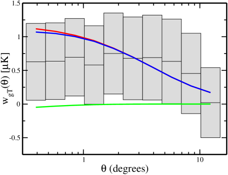
Figure 3: The comparison of our theoretical predictions to our measurement of the W-channel WMAP map cross-correlated with the $z\sim 0.49$ galaxy subsample. The fitted ISW cross-correlation function is given by the red line, the SZ by the green line and the sum of the two is given by the blue line. We find $\bar{b}=5.47\pm 1.82$ and $\overline{T_{\rm e}b_{\rm P}}=0.15\pm 0.61$, where the errors are unmarginalized.

VI Conclusions

We present here measurements of the cross-correlation function between the currently available SDSS galaxy data and the WMAP CMB maps of the sky. The individual measurements in Figure 2 are significant at the $>90\%$ confidence, while FDR strongly rejects the null hypothesis. The achromatic nature of the signal (in the Q, V, and W frequency channels) confirms the signal is of cosmological origin. Our results are consistent with the NVSS-CMB correlations(Boughn & Crittenden, 2003; Nolta et al., 2003), but may be harder to reconcile with other optical–CMB measurements of the ISW effect(Fosalba & Gaztañaga, 2003; Myers2003, ). These results are consistent with the predicted ISW effect (which is largely independent of dark energy properties) and a minor SZ contribution. Assuming a flat universe, our detection of the ISW effect provides independent physical evidence for the existence of dark energy. In future papers, analyzing all available SDSS data, we will present a more detailed comparison between the theoretical models and the data, as well consistency checks of the observed correlation amplitude with galaxy biases and dark energy models.

- (1) Abazajian, K., et al. 2003, astro-ph/0305492
- Bennett et al. (2003) Bennett, C.L. et al. 2003, astro-ph/0302207
- Birkinshaw (1999) Birkinhshaw, M. 1991, Phys.Rep., 310, 97.
- Boughn & Crittenden (2003) Boughn, S. P. & Crittenden, R. G. 2003, astro-ph/0305001
- Budavári et al. (2000) Budavári, T., Szalay, A. S., Connolly, A. J., Csabai, I., & Dickinson, M. 2000, AJ, 120, 1588
- (6) Caldwell, R. R., Dave, R., & Steinhardt, P. J. 1998, Physical Review Letters, 80, 1582
- Coble, Dodelson, & Frieman (1997) Coble, K., Dodelson, S., & Frieman, J. A. 1997, Phys ReV D, 55, 1851
- Corasaniti et al. (2003) Corasaniti, P.S. et al. 2003, Phys.Rev.Lett. 90, 091303
- Cooray (2002) Cooray, A. 2002, Phys. Rev. D, 65, 083518.
- Eisenstein et al. (2001) Eisenstein, D. J. et al. 2001, AJ, 122, 2267
- Fosalba & Gaztañaga (2003) Fosalba P., Gaztañaga E., Castander, F. J. 2003, astro-ph/0307249
- (12) Fukugita, M., Ichikawa, T., Gunn, J.E., Doi, M., Shimasaku, K., & Schneider, D.P. 1996, AJ, 111,1748
- (13) Gorski, K.M., Hivon, E., & Wandelt, B.D. 1999,in Proceedings of the MPA/ESO Cosmology Conference “Evolution of Large-Scale Structure”, eds A.J.Banday, R.S.Sheth, and L. Da Costa, Printpartners Ipskamp, NL, pp 37-42.
- (14) Gunn, J. E. et al. 1998,AJ, 116, 3040
- (15) Hogg, D.W., Finkbeiner, D.P., Schlegel, D.J., and Gunn, J.E. 2001, AJ, 122, 2129
- (16) Hopkins, A. M., Miller, C. J., Connolly, A. J., Genovese, C., Nichol, R. C., & Wasserman, L. 2002, AJ, 123, 1086
- Hu & Dodelson (2002) Hu, W. & Dodelson, S. 2002, ARA&A, 40, 171.
- Hu, Seljak, White, & Zaldarriaga (1998) Hu, W., Seljak, U., White, M., & Zaldarriaga, M. 1998, Phys ReV D, 57, 3290
- (19) Miller, C. et al. 2001, AJ, 122, 3492
- (20) Myers, A.D., Shanks, T. Outram, P.J., Wolfendale, A.W. 2003, astro-ph/0306180
- Nolta et al. (2003) Nolta, M. R. et al. 2003, astro-ph/0305097
- Peiris & Spergel (2000) Peiris. H., Spergel, D.N. 2000, ApJ, 540, 605
- (23) Pier, J.R., Munn, J.A., Hindsley, R.B., Hennessy, G.S., Kent, S.M., Lupton, R.H., and Ivezic, Z. 2003, AJ, 125, 1559
- Sachs & Wolfe (1967) Sachs, R. K. & Wolfe, A. M. 1967, ApJ, 147, 73
- Scranton et al. (2002) Scranton, R. et al. 2002, ApJ, 579, 48
- (26) Smith, J.A., et al 2002, AJ, 123, 2121
- Spergel et al. (2003) Spergel, D.N. et al. 2003, astro-ph/0302209.
- (28) Stoughton, C., et al 2002, AJ, 123, 485
- Szapudi, Prunet, & Colombi (2001) Szapudi, I., Prunet, S., & Colombi, S. 2001, Ap. J. Let. , 561, L11
- Tegmark et al. (2003) Tegmark, M., et al. 2003, astro-ph/0302496.
- York et al. (2000) York, D.G. et al. 2000, Astron. J., 120, 1579.
- Zel’dovich & Sunyaev (1967) Zel’dovich Y.B., & Sunyaev, R.A. 1967, ApSpSci, 4, 301.