The dependence on environment of the color–magnitude relation of galaxies

Abstract

The distribution in color and absolute magnitude is presented for 55,158 galaxies taken from the Sloan Digital Sky Survey in the redshift range $0.08<z<0.12$, as a function of galaxy number overdensity in a line-of-sight cylinder of transverse radius $1~{}h^{-1}\,\mathrm{Mpc}$. In all environments, bulge-dominated galaxies (defined to be those with radial profiles best fit with large Sérsic indices) form a narrow, well defined color–magnitude relation. Although the most luminous galaxies reside preferentially in the highest density regions, there is only a barely detectable variation in the color (zero-point) or slope of the color–magnitude relation ($<0.02~{}\mathrm{mag}$ in ${}^{0.1}[g-r]$ or $[B-V]$). These results constrain variations with environmental density in the ages or metallicities of typical bulge-dominated galaxies to be under 20 percent.

1 Introduction

Red, bulge-dominated galaxies show many precise regularities, including narrow, mass-dependent distributions of colors, surface-brightnesses, radial profile shapes, ages, chemical abundances, velocity dispersions, and mass-to-light ratios (e.g., Baum, 1959; Faber, 1973; Faber & Jackson, 1976; Visvanathan & Sandage, 1977; Djorgovski & Davis, 1987; Dressler et al., 1987; Kormendy & Djorgovski, 1989; Roberts & Haynes, 1994; Burstein et al., 1997; Terlevich et al., 2001; Eisenstein et al., 2003; Bernardi et al., 2003a, b, c; Blanton et al., 2003a). The most massive of these bulge-dominated galaxies reside preferentially in the most dense environments, and especially in rich clusters of galaxies (Dressler, 1980; Postman & Geller, 1984); indeed the most massive red galaxy populations have the highest average environmental overdensities (Hogg et al., 2003).

Are these trends, i.e., the relationships between mass and environment and between mass and everything else, related? In this Letter we look at the color–magnitude relationship of red, bulge-dominated galaxies as a function of environment.

Generically, in models in which structure grows gravitationally, the most dense regions of the Universe will have collapsed earlier and will contain the most massive objects. Detailed modeling of galaxy formation in current cosmological simulations bears this out; galaxies in very high density regions are predicted to be more luminous and more red (older) than those in typical density regions (e.g., Cen & Ostriker, 1993; Kauffmann et al., 1993; Kauffmann, 1996; Kauffmann et al., 1999; Benson et al., 2000; Diaferio et al., 2001). While these models predict morpholgy, color, and luminosity variations with overdensity, it is not clear whether they predict color differences at fixed morphology and luminosity.

The Sloan Digital Sky Survey (SDSS) is the best available data set for work on these questions, because of its sample size, high signal-to-noise imaging, sky coverage, and complete spectroscopy (e.g., York et al., 2000). Indeed, the SDSS has already made some progress on related issues, including the dependence of clustering on luminosity and color (Zehavi et al., 2002), the star-formation rate as a function of environment (Gomez et al., 2003), the mean red-galaxy spectrum as a function of environment (Eisenstein et al., 2003), and the mean galaxy environment as a function of color and luminosity (Hogg et al., 2003; Blanton et al., 2003a).

In what follows, a cosmological world model with $(\Omega_{\mathrm{M}},\Omega_{\mathrm{\Lambda}})=(0.3,0.7)$ is adopted, and the Hubble constant is parameterized $H_{0}=100\,h~{}\mathrm{km\,s^{-1}\,Mpc^{-1}}$, for the purposes of calculating distances and volumes (e.g., Hogg, 1999).

2 Data

The SDSS is taking $ugriz$ CCD imaging of $10^{4}~{}\mathrm{deg^{2}}$ of the Northern Galactic sky, and, from that imaging, selecting $10^{6}$ targets for spectroscopy, most of them galaxies with $r<17.77~{}\mathrm{mag}$ (e.g., Gunn et al., 1998; York et al., 2000; Stoughton et al., 2002). All the data processing: astrometry (Pier et al., 2003), source identification, deblending and photometry (Lupton et al., 2001), calibration (Fukugita et al., 1996; Smith et al., 2002), spectroscopic target selection (Eisenstein et al., 2001; Strauss et al., 2002; Richards et al., 2002), spectroscopic fiber placement (Blanton et al., 2003), and spectroscopic data reduction are performed with automated SDSS software. Redshifts are measured on the reduced spectra by an automated system, which models each galaxy spectrum as a linear combination of stellar populations (Schlegel, in preparation).

To each galaxy’s extracted radial profile, a seeing-corrected Sérsic model is fit (as in Blanton et al., 2003a). The Sérsic model is that surface brightness $I$ is proportional to $\exp(-r/r_{0})^{1/n}$, where $r$ is the angular radius from the galaxy center, $r_{0}$ is a characteristic radius, and $n$ is a free parameter known as the “Sérsic index”. Galaxies with more concentrated radial profiles have larger $n$; an exponential disk has $n=1$ and a de Vaucouleurs profile has $n=4$.

Galaxy luminosities (absolute magnitudes) and colors (measured by the standard SDSS petrosian technique; Petrosian, 1976) are computed in fixed bandpasses, using Galactic extinction corrections (Schlegel et al., 1998) and $K$ corrections (computed with kcorrect v1_11; Blanton et al., 2003). Galaxy magnitudes are $K$ corrected not to the redshift $z=0$ observed bandpasses but to bluer bandpasses ${}^{0.1}g$, ${}^{0.1}r$ and ${}^{0.1}i$ “made” by shifting the SDSS $g$, $r$, and $i$ bandpasses to shorter wavelengths by a factor of 1.1 (as in Blanton et al., 2003, 2003a). This means that galaxies at redshift $z=0.1$ have trivial (but not zero; Hogg et al., 2002) $K$ corrections. The full error analysis of SDSS photometry is not complete, but scatter in the $g$, $r$, and $i$ band magnitudes appears to be better than $0.03~{}\mathrm{mag}$ (RMS).

For a red galaxy, ${}^{0.1}[g-r]$ (calibrated to the AB magnitude system) can be converted approximately to $[B-V]$ with

$$\displaystyle\left[B-V\right]_{\mathrm{AB}} = 0.83\,\,^{0.1}\left[g-r\right]-\left[0.025~{}\mathrm{mag}\right]$$

$$\left[B-V\right]_{\mathrm{AB}} = \left[B-V\right]_{\mathrm{Vega}}-\left[0.115~{}\mathrm{mag}\right]\quad,$$ (1)

where the subscripts indicate AB or Vega-relative calibration. This transformation is robust because the ${}^{0.1}g$ and ${}^{0.1}r$ bandpasses are very close to $B$ and $V$ in effective wavelength.

The sample of galaxies used here is a subset of an SDSS statistical sample known as “NYU LSS sample12”, further selected to have apparent magnitude in the range $14.5<r<17.77~{}\mathrm{mag}$, and redshift in the narrow range $0.08<z<0.12$. These cuts left 55,158 galaxies.

The sample is statistically complete, with small incompletenesses coming primarily from (1) galaxies missed because of mechanical spectrograph constraints ($\sim 7$ percent; Blanton et al., 2003), which does lead to a slight under-representation of high-density regions, and (2) spectra in which the redshift is either incorrect or impossible to determine ($<1$ percent). In addition, there are some galaxies ($\sim 1$ percent) blotted out by bright Galactic stars, but this incompleteness should be uncorrelated with galaxy properties.

For each galaxy in the sample there is a computed inverse selection volume $1/V_{\mathrm{max}}$, where $V_{\mathrm{max}}$ is the total comoving volume in which the galaxy could lie and still be included in the sample, accounting for the flux limits, surface brightness limits, redshift limits, and completeness as a function of angle (as in Blanton et al., 2003a).

We employ an environment overdensity estimate $\delta_{1\times 8}$ based on the SDSS spectroscopic sample; it is a measure of the three-dimensional redshift-angle space number density excess around each galaxy. The comoving transverse distances and comoving line-of-sight distances (e.g., Hogg, 1999) are computed between each spectroscopic galaxy and its neighboring spectroscopic galaxies (not attempting to correct for peculiar velocities). For each galaxy, neighbors within a cylinder with a transverse comoving radius of $1\,h^{-1}~{}\mathrm{Mpc}$ and a comoving half-length of $8\,h^{-1}~{}\mathrm{Mpc}$ in this space are counted; the result is divided by the no-clustering prediction made from the galaxy luminosity function (Blanton et al., 2003b) and the sample selection critera, and unity is subtracted to produce the overdensity estimate $\delta_{1\times 8}$. A galaxy in an environment with the cosmic mean density has $\delta_{1\times 8}=0$. The statistical properties of the estimator $\delta_{1\times 8}$ vary with redshift because the density of the sample varies with redshift, but the sample considered here is selected to be only in the narrow redshift interval $0.08<z<0.12$. It is worthy of note that even galaxies with $\delta_{1\times 8}>50$ (the highest density subsample used below) are not found exclusively inside the cores of rich clusters.

3 Results

Figure 1 shows the distribution in color and magnitude for the entire sample, and subsamples chosen to lie in low density regions ($\delta_{1\times 8}<3.0$), high density regions ($\delta_{1\times 8}>7.0$), and very high density regions ($\delta_{1\times 8}>50$), and subsamples chosen to have low Sérsic index ($n<2.0$) and high Sérsic index ($n>2.0$). Overplotted on all panels is the same color–magnitude relation, a linear fit to the dependence of color on magnitude for the all-environment, high Sérsic subsample, with sigma-clipping at $2\,\sigma$ in the color direction. The apparent bimodality of the galaxy population in Figure 1 and the value of the Sérsic index for separating populations has been made evident previously (Blanton et al., 2003a).

The distribution of galaxies is different in the different subsamples. The most striking difference is that the bulge-dominated ($n>2.0$) galaxies are much redder than the disk-dominated galaxies. Another striking difference is that the bulge-dominated galaxies are over-represented in the higher density regions. Another is that the very most luminous ($M_{{}^{0.1}i}\sim-22.8~{}\mathrm{mag}$) galaxies are over-represented in the higher density regions.

Among the bulge-dominated ($n>2.0$) galaxies it is just as striking that the color–magnitude relation is independent of the environmental overdensity. There are environmental differences in the distribution of galaxies in the color–magnitude plane, but the most likely color for a bulge-dominated galaxy of any given luminosity is not much redder in the highest density environments than it is in the lowest.

Figure 2 shows the color-direction residuals away from the linear fit, for the high Sérsic-index galaxies in low, high, and very high density regions. The distributions differ in the abundance of blue galaxies (and therefore in the shape of the residual distribution), as noted previously (Pimbblet et al., 2002; Kuntschner et al., 2002). All three overdensity subsamples show strong red peaks, with similar modes and dispersions. In detail, the highest density subsample shows the narrowest and reddest peak, with a mode that is slightly redder (by $<0.02~{}\mathrm{mag}$ in ${}^{0.1}[g-r]$) than that of the lowest density subsample.

This independence of red galaxy colors on environment is consistent with a previous SDSS result (Bernardi et al., 2003c) which was based on a restricted sample of early-type galaxies, selected on the basis of radial profile, ellipticity, color, and lack of emission lines. Small variations with environmental density have been found in the mean strengths of narrow spectral features in red galaxies (Eisenstein et al., 2003), but evidently they are not strong enough to affect the broad-band colors significantly.

There are several other trends visible in Figure 1. The bulge-dominated galaxies show a larger “tail” of blue outliers in lower density regions; some of the galaxies in this tail are post-starburst galaxies (Quintero et al., 2003); some of the others are LINERs (work in preparation). The high-density regions contain a small population of red, exponential, sub-$L^{\ast}$ galaxies ($L^{\ast}$ is at $M_{{}^{0.1}i}\approx-20.8~{}\mathrm{mag}$, Blanton et al., 2003b) not seen at lower densities. This population is visible in previous SDSS work (Hogg et al., 2003).

The slope (color over absolute magnitude) of the color-magnitude relation plotted in Figure 1 is $-0.022~{}\mathrm{mag\,mag^{-1}}$, and the HWHM of the relation visible in Figure 2 is $<0.05~{}\mathrm{mag}$ (expressed as a limit because calibration errors may contribute significantly). If high luminosity red galaxies are made from the mergers of lower luminosity galaxies without further star formation, the color-magnitude relation is difficult to explain. On the other hand, the major merger of two equal-luminosity galaxies on the color–magnitude relation does not, by itself, create a noticeable outlier in this dataset.

The fact that the distribution of bulge-dominated galaxy luminosities is a strong function of environment is emphasized in Figure 3, which shows the luminosity distributions of the high Sérsic ($n>2.0$) galaxies in the three environment subsamples. The abundance of high luminosity galaxies increases rapidly with environmental overdensity. This increase in average luminosity with increasing overdensity is related to (but not identical with) the previously shown increase in average overdensity with increasing luminosity (i.e., the converse relation) for these galaxies (Hogg et al., 2003).

A change of $\sim 0.01~{}\mathrm{mag}$ in ${}^{0.1}[g-r]$ corresponds to $\sim 0.8~{}\mathrm{Gyr}$ of aging or $\sim 0.04~{}\mathrm{dex}$ in metallicity for an old ($\sim 10~{}\mathrm{Gyr}$), solar metallicity stellar population (e.g., Charlot et al., 2003). Of course it is possible that there are compensating effects between metallicity and age (e.g., Kuntschner et al., 2002), although no evidence for such a trade-off appears in the analysis of SDSS spectra; what appears is evidence that small age effects, small metallicity effects, and small relative abundance effects (e.g., alpha enhancement) all come in at comparable levels (Eisenstein et al., 2003).

It is difficult to imagine how high and low density regions of the Universe can evolve in their different ways without affecting the color–magnitude relation of the bulge-dominated galaxy population, in color or slope, by more than what is observed here.

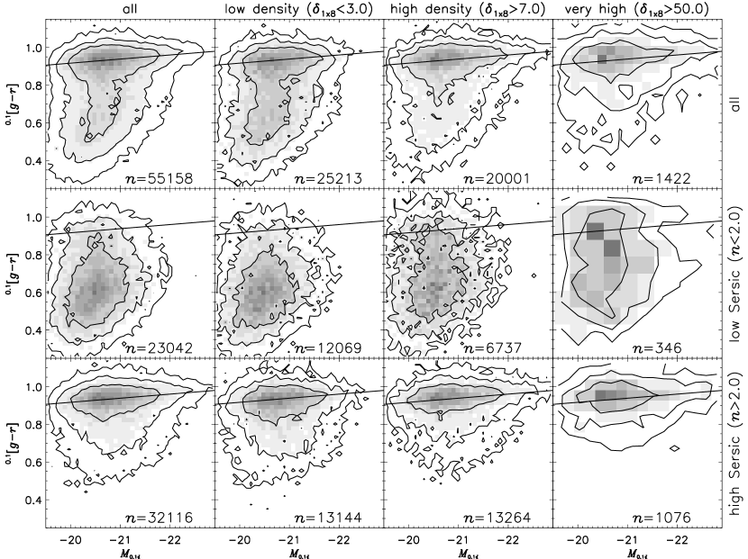
Figure 1: The top left panel shows the distribution in absolute magnitude $M_{{}^{0.1}i}$ in the ${}^{0.1}i$ band and ${}^{0.1}[g-r]$ color for the entire sample. The columns show subsamples cut in overdensity $\delta_{1\times 8}$ (a mean density environment has $\delta_{1\times 8}=0$). The rows show subsamples cut in Sérsic index $n$ (an exponential disk has $n=1$ and a de Vaucouleurs profile has $n=4$). In each panel, the greyscale monotonically represents the abundance of sample galaxies in the two-dimensional space of color and magnitude and the contours enclose 52.0, 84.3, and 96.6 percent of the sample. This represents properties of the sample; the data have not been weighted by $1/V_{\mathrm{max}}$. Overplotted on all panels is the same straight, solid line showing the best-fit color–magnitude relation from the lower-left panel, fit as described in the text.

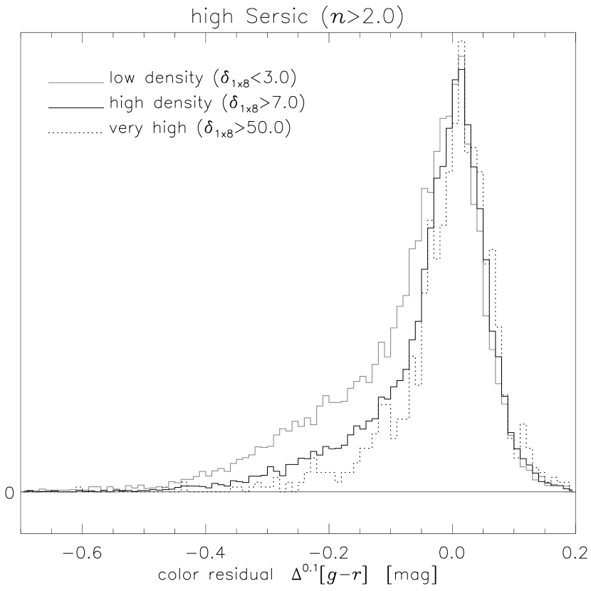
Figure 2: The distribution of color residuals (observed minus fit) relative to the linear fit plotted in Figure 1 for the high sersic samples at low and high density. The histograms have been arbitrarily re-normalized to have similar peak heights.

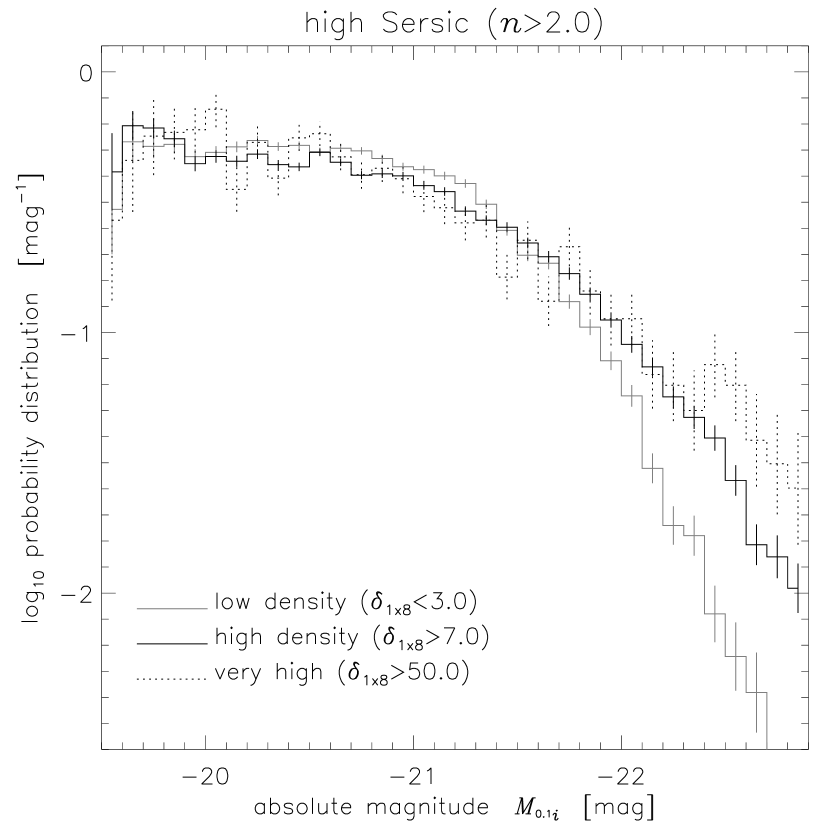
Figure 3: The $1/V_{\mathrm{max}}$-weighted distribution function of galaxy absolute magnitudes for the high Sérsic ($n>2.0$) galaxies for the different density environments. The error bars show Poisson uncertainties only.

References

- Baum (1959) Baum, W. A. 1959, PASP, 71, 106
- Benson et al. (2000) Benson, A. J., Baugh, C. M., Cole, S., Frenk, C. S., & Lacey, C. G. 2000, MNRAS, 316, 107
- Bernardi et al. (2003a) Bernardi, M. et al. 2003a, AJ, 125, 1849
- Bernardi et al. (2003b) Bernardi, M. et al. 2003b, AJ, 125, 1866
- Bernardi et al. (2003c) Bernardi, M. et al. 2003c, AJ, 125, 1882
- Blanton et al. (2003) Blanton, M. R., Brinkmann, J., Csabai, I., Doi, M., Eisenstein, D. J., Fukugita, M., Gunn, J. E., Hogg, D. W., & Schlegel, D. J. 2003, AJ, 125, 2348
- Blanton et al. (2003) Blanton, M. R., Lin, H., Lupton, R. H., Maley, F. M., Young, N., Zehavi, I., & Loveday, J. 2003, AJ, 125, 2276
- Blanton et al. (2003a) Blanton, M. R. et al. 2003a, ApJ, in press (astro-ph/0209479)
- Blanton et al. (2003b) Blanton, M. R. et al. 2003b, ApJ, in press (astro-ph/0210215)
- Burstein et al. (1997) Burstein, D., Bender, R., Faber, S., & Nolthenius, R. 1997, AJ, 114, 1365
- Cen & Ostriker (1993) Cen, R. & Ostriker, J. P. 1993, ApJ, 417, 415
- Charlot et al. (2003) Charlot, S. et al. 2003, MNRAS, in press
- Diaferio et al. (2001) Diaferio, A., Kauffmann, G., Balogh, M. L., White, S. D. M., Schade, D., & Ellingson, E. 2001, MNRAS, 323, 999
- Djorgovski & Davis (1987) Djorgovski, S. & Davis, M. 1987, ApJ, 313, 59
- Dressler (1980) Dressler, A. 1980, ApJ, 236, 351
- Dressler et al. (1987) Dressler, A., Lynden-Bell, D., Burstein, D., Davies, R. L., Faber, S. M., Terlevich, R., & Wegner, G. 1987, ApJ, 313, 42
- Eisenstein et al. (2001) Eisenstein, D. J. et al. 2001, AJ, 122, 2267
- Eisenstein et al. (2003) Eisenstein, D. J. et al. 2003, ApJ, 585, 694
- Faber (1973) Faber, S. M. 1973, ApJ, 179, 731
- Faber & Jackson (1976) Faber, S. M. & Jackson, R. E. 1976, ApJ, 204, 668
- Fukugita et al. (1996) Fukugita, M., Ichikawa, T., Gunn, J. E., Doi, M., Shimasaku, K., & Schneider, D. P. 1996, AJ, 111, 1748
- Gomez et al. (2003) Gomez, P. et al. 2003, ApJ, 584, 210
- Gunn et al. (1998) Gunn, J. E., Carr, M. A., Rockosi, C. M., Sekiguchi, M., et al. 1998, AJ, 116, 3040
- Hogg (1999) Hogg, D. W. 1999, astro-ph/9905116
- Hogg et al. (2002) Hogg, D. W., Baldry, I. K., Blanton, M. R., & Eisenstein, D. J. 2002, astro-ph/0210394
- Hogg et al. (2003) Hogg, D. W., Blanton, M. R., Eisenstein, D. J., Gunn, J. E., Schlegel, D. J., Zehavi, I., Bahcall, N. A., Brinkmann, J., Csabai, I., Schneider, D. P., Weinberg, D. H., & York, D. G. 2003, ApJ, 585, L5
- Kauffmann (1996) Kauffmann, G. 1996, MNRAS, 281, 487
- Kauffmann et al. (1999) Kauffmann, G., Colberg, J. M., Diaferio, A., & M., W. S. D. 1999, MNRAS, 303, 188
- Kauffmann et al. (1993) Kauffmann, G., White, S. D. M., & Guiderdoni, B. 1993, MNRAS, 264, 201
- Kormendy & Djorgovski (1989) Kormendy, J. & Djorgovski, S. 1989, ARA&A, 27, 235
- Kuntschner et al. (2002) Kuntschner, H., Smith, R. J., Colless, M., Davies, R. L., Kaldare, R., & Vazdekis, A. 2002, MNRAS, 337, 172
- Lupton et al. (2001) Lupton, R. H., Gunn, J. E., Ivezić, Z., Knapp, G. R., Kent, S., & Yasuda, N. 2001, in ASP Conf. Ser. 238: Astronomical Data Analysis Software and Systems X, Vol. 10, 269–??
- Petrosian (1976) Petrosian, V. 1976, ApJ, 209, L1
- Pier et al. (2003) Pier, J. R., Munn, J. A., Hindsley, R. B., Hennessy, G. S., Kent, S. M., Lupton, R. H., & Ivezić, Ž. 2003, AJ, 125, 1559
- Pimbblet et al. (2002) Pimbblet, K. A., Smail, I., Kodama, T., Couch, W. J., Edge, A. C., Zabludoff, A. I., & O’Hely, E. 2002, MNRAS, 331, 333
- Postman & Geller (1984) Postman, M. & Geller, M. 1984, ApJ, 281, 95
- Quintero et al. (2003) Quintero, A. D., Hogg, D. W., (NYU), M. R. B., Schlegel, D. J., Eisenstein, D. J., Gunn, J. E., Brinkmann, J., Fukugita, M., Glazebrook, K., & Goto, T. 2003, ApJ, submitted (astro-ph/0307074)
- Richards et al. (2002) Richards, G. et al. 2002, AJ, 123, 2945
- Roberts & Haynes (1994) Roberts, M. S. & Haynes, M. P. 1994, ARA&A, 32, 115
- Schlegel et al. (1998) Schlegel, D. J., Finkbeiner, D. P., & Davis, M. 1998, ApJ, 500, 525
- Smith et al. (2002) Smith, J. A., Tucker, D. L., et al. 2002, AJ, 123, 2121
- Stoughton et al. (2002) Stoughton, C. et al. 2002, AJ, 123, 485
- Strauss et al. (2002) Strauss, M. A. et al. 2002, AJ, 124, 1810
- Terlevich et al. (2001) Terlevich, A. I., Caldwell, N., & Bower, R. G. 2001, MNRAS, 326, 1547
- Visvanathan & Sandage (1977) Visvanathan, N. & Sandage, A. 1977, ApJ, 216, 214
- York et al. (2000) York, D. et al. 2000, AJ, 120, 1579
- Zehavi et al. (2002) Zehavi, I. et al. 2002, ApJ, 571, 172