Photon counting strategies with low light level CCDs

Abstract

Low light level charge coupled devices (L3CCDs) have recently been developed, incorporating on-chip gain. They may be operated to give an effective readout noise much less than one electron by implementing an on-chip gain process allowing the detection of individual photons. However, the gain mechanism is stochastic and so introduces significant extra noise into the system. In this paper we examine how best to process the output signal from an L3CCD so as to minimize the contribution of stochastic noise, while still maintaining photometric accuracy.

We achieve this by optimising a transfer function which translates the digitised output signal levels from the L3CCD into a value approximating the photon input as closely as possible by applying thresholding techniques. We identify several thresholding strategies and quantify their impact on photon counting accuracy and effective signal-to-noise.

We find that it is possible to eliminate the noise introduced by the gain process at the lowest light levels. Reduced improvements are achieved as the light level increases up to about twenty photons per pixel and above this there is negligible improvement. Operating L3CCDs at very high speeds will keep the photon flux low, giving the best improvements in signal-to-noise ratio.

This is a preprint of an Article accepted for publication in Monthly Notices of the Royal Astronomical Society ©2003 The Royal Astronomical Society.

1 Introduction

Charge coupled devices (CCDs) are ideal detectors in many astronomical applications. They are available in large-format arrays, have high quantum efficiency (QE), a linear response, and, if cooled sufficiently, a very low dark current. Their major shortcoming is readout noise, i.e. the additional noise added by the on-chip output amplifier, where the charge of the detected photo-electrons is converted into an output voltage. Currently, the typical noise levels achieved at slow readout rates (e.g. kHz pixel rates) are little better than $\sim 2$ electrons per read (Jerram et al., 2001). At the higher readout rates (MHz pixel rates) often used, for example, for adaptive optics and interferometric applications, far poorer performance is the norm, with typical noise levels of $\sim 10-100$ electrons per readout (Jerram et al., 2001).

A novel solution to this problem, in which on-chip gain is used to amplify the signal prior to readout, has recently been demonstrated by E2V Technologies (formerly Marconi Applied Technologies, Jerram et al. (2001)). In this approach, an extended serial register is used to allow electron avalanche multiplication so that a large mean gain can be realised prior to a conventional readout amplifier. Although the effective gain can be very large, the detailed process by which the signal is amplified is stochastic and so introduces additional noise at the output. The effects of this noise, and its correction by a judicious analysis of the output from a typical low light level CCD (hereafter L3CCD) are the primary subjects of this paper.

The content of the paper is as follows. In Section 2 we describe how the L3CCD works and develop a numerical and probabilistic model of the gain mechanism. In Section 3 we discuss techniques for analysing the noisy output signal of an L3CCD and the implications for photometric accuracy and signal-to-noise ratio (SNR), and we conclude in Section 4.

2 Characteristics of the L3CCD

2.1 Principles of L3CCD Operation

The L3CCD architecture is similar to that of a normal CCD except that it has extended serial register, called the multiplication register, allowing for additional serial transfers before the signal reaches the ouput amplifier (see Fig. 1). The electrode voltages in the multiplication register can be adjusted so that avalanche multiplication of the electrons occurs as they are moved through each element of this part of the device. At each step, the probability, $p$, of producing an additional electron per initial input electron is small — typically this may be $0.01-0.02$ — but the cumulative effect of many transfers can be very large. For example, for a register comprising $r=591$ elements (the number of elements in the CCD65 from E2V Technologies), the mean gain, $g$, will be $\left(1+p\right)^{r}=6629$, when $p=0.015$.

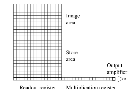
Figure 1: A schematic diagram of an L3CCD showing the multiplication register.

In general, the probability distribution of the output $x$, for an input of $n$ (integer) photo-electrons, where the mean gain is $g$ will be given approximately by (Appendix A and Fig. 2)

$$p\left(x\right)=\frac{x^{n-1}\exp(-x/g)}{g^{n}\left(n-1\right)!}$$ (1)

when the photon input level is relatively small and the gain is large. This distribution has a mean of $ng$ and a variance of $ng^{2}$ and at high light levels is approximately Gaussian. The signal noise introduced by this multiplication process is independent of the photon input. The SNR of an L3CCD output is obtained by combining in quadrature the noise due to the Poisson nature of light with the noise from the multiplication process. At a mean light level $\mu$ photons per pixel, this gives an SNR equal to $\sqrt{\mu}/E$ where $E$ (the excess noise factor, hereafter ENF) is equal to $\sqrt{2}$ for an L3CCD output with large gain. The nature of the multiplication process means that in general there will not be a one-to-one mapping between the number of electrons entering and leaving the multiplication register (see Fig. 2), so that in principle there will be always be some uncertainty when estimating the input flux. For a CCD with no gain, $E$ is equal to unity, and so to achieve the same SNR when using a large gain, we will need to detect twice as many photons, meaning that the multiplication process has effectively halved the QE of the device. This is a serious loss as astronomers are happy to spend a lot of money on optical coatings to increase system throughput by only a few percent, and do not want to accept the loss in effective QE that the use of an L3CCD implies. To be able to increase the effective QE using signal processing is therefore essential if L3CCDs are to be used effectively for astronomy. This is the main driving force behind our investigation, which aims to use our additional knowledge of the system to allow us to reduce the uncertainty in the measured fluxes.

Figure 2: L3CCD output probability distribution for a given photon input. Inputs of $1-4$ photons are shown for a mean gain of 6629. Note the significant overlap between different inputs which causes uncertainties when estimating the input from the output.

2.2 Reducing the noise

We consider processing strategies which allow up to minimize the stochastic multiplication noise. At very low light levels, much less than one detected photon per imaging pixel, we are able to use the L3CCD in a photon counting mode. At these low light levels, we will either get zero or one photons in a pixel per integration time. This will then result in either a signal much smaller than the amplifier read noise (zero photons), or when a detected photo-electron is amplified, a much larger signal. Provided the mean multiplication gain is much greater than the read noise, we can then treat any signal above some threshold as having arisen from one photon event. Replacing the range of signals we get from a pixel containing one photon (curve 1 in Fig. 2) eliminates the variance in output signal introduced by the multiplication process of the L3CCD and increases the SNR to a value we expect from a conventional CCD with negligible read-out noise.

At higher light levels this technique will not work, since coincidence losses (more than one photon falling on a pixel, being interpreted as one photon) will become increasingly important. Nevertheless, the idea of thresholding can still be helpful if we use more than one threshold. We can see how this might work as follows. An L3CCD with a mean multiplication gain of $g$ might give an output signal of $fg$. This could be due to a single detected photon that has been amplified by an unusually large amount. Alternatively, if we set thresholds $T_{n}$ and $T_{n+1}$ and estimate the flux to be $n$ detected photo-electrons before multiplication if the detected signal satisfies $T_{n}\leq fg<T_{n+1}$, then we will be able to maximize our chance of estimating the flux correctly if we choose thresholds correctly. It is the determination of these threshold levels and any corrections that need to be applied in order to conserve flux which we now consider, together with their impact on the L3CCD output SNR.

2.3 Thresholding schemes

We have considered many different signal-processing strategies, and provide details of the most useful selection here. We investigate which of these provide the largest SNR improvement. When investigating these strategies, we assume that the data is first thresholded at some level above the on-chip readout noise level (typically $6\sigma$ where $\sigma$ is the RMS noise due to the readout amplifier) so that amplifier read noise is negligible. Following this, the strategies considered are:

1. Analogue:

The output signal is divided by the mean gain.

2. Photon Counting (PC):

If the output signal is above a single fixed noise threshold it is treated as representing one input photon.

3. Poisson Probability (PP):

Threshold levels are set where the probability of an output resulting from a mean input of $n$ Poisson photons is equal to the probability of the output resulting from a mean input of $n+1$ Poisson photons.

The Photon Counting (PC) thresholding strategy will underestimate flux at light levels where there is a non-zero probability of more than one photon being detected on a single pixel. The Poisson Probability (PP) strategy will overestimate the flux, particularly at low light levels, and so a theoretically determined correction is necessary after the detections, which we investigate in section 3.

2.3.1 Threshold boundaries

At a given mean light level, $\mu$ photons per pixel, the L3CCD output with mean gain $g$ can be estimated by providing the photon input in Eq. 1 with a Poisson probability distribution, giving:

$$p\left(x,\mu\right)=\sum_{n=1}^{\infty}\frac{\exp\left(-\mu-x/g\right)\mu^{n}(x/g)^{n-1}}{g(n-1)!n!}$$ (2)

where $p\left(x,\mu\right)$ is the probability that the L3CCD output will be $x$ when the mean light level is $\mu$, and the mean gain is $g$.

We use this distribution to determine threshold boundaries for the PP thresholding strategy, which are given in Table 1. These are placed at the points where the probability of getting an output $x$ with a mean light level $\mu$ is equal to the probability of getting the same output $x$ with a mean light level of $\mu+1$ as shown in Fig. 3, i.e. finding $x$ such that

$$p\left(x,a\right)=p\left(x,a+1\right)$$ (3)

where the $a^{\mathrm{th}}$ threshold boundary is placed at position $x$, and $p\left(x,a\right)$ is defined in Eq. 2. This results in threshold boundary positions independent of the mean light level. The theoretically predicted mean flux and ENF arising from this strategy is also calculated.

Table 1: Threshold boundaries in units of mean gain, for a PP thresholding strategy.

Threshold	Boundary	Threshold	Boundary
1	0.71	7	6.97
2	1.89	8	7.98
3	2.93	9	8.98
4	3.95	10	9.98
5	4.96	11	11.0
6	5.97	$n\geq 11$	$n$

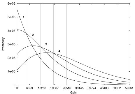
Figure 3: The L3CCD output probability distribution for mean (Poisson) light levels of 1 (left curve) to 4 (right curve) photons per pixel, as given by Eq. 2. Threshold boundaries for the PP thresholding strategy are placed where these curves cross.

2.4 Threshold evaluation

Monte-Carlo simulations were used to verify that our threshold positions were chosen correctly, and that our calculations of photon input estimation and ENF were correct. Input photon streams were generated for differing mean light levels assuming Poisson statistics, and were injected into the first pixel of a multiplication register of length $r$. The transfer of this signal to the next pixel of the register was then computed assuming a probability $p$ that any given photo-electron would be amplified to give 2 photo-electrons, and a probability $1-p$ that the transfer took place with no amplification. This process was then repeated a further $r-1$ times to simulate the output expected for the initial input signal. In this way, the expected output for L3CCDs with differing multiplication probabilities and register lengths could easily be generated for differing input light levels and threshold boundary positions. Large numbers of these output data sequences were then processed to verify that the theoretical ENF and flux estimation calculations were correct.

2.5 Figures of merit

In order to assess the performance of different signal-processing strategies, the quality of the signal recovery was quantified using both the ENF and the following misfit function, $M$:

$$M=\frac{\sum_{\mathrm{i}}\left(n_{\mathrm{i}}-y_{\mathrm{i}}\right)^{2}}{\sum_{\mathrm{i}}n_{\mathrm{i}}},$$ (4)

where $n_{\mathrm{i}}$ is the true input photon count and $y_{\mathrm{i}}$ the value of the input signal estimated from the thresholded L3CCD output, $x_{\mathrm{i}}$. Data sequences comprising many tens of thousands of signal values were generated so as to allow different methods for generating the estimates $\{y_{\mathrm{i}}\}$ from the raw L3CCD outputs $\{x_{\mathrm{i}}\}$. The minimization of this misfit function corresponds to the best input prediction.

An ideal detector will give a misfit of $M=0$, and a variance equal to the variance of the input (Poisson) data, $\mu=\overline{n}$, with the SNR equal to $\sqrt{\mu}$. A non-ideal detector will have greater dispersion in the output, resulting in a reduced SNR of $\sqrt{\mu}/E$ where $E$ is the ENF.

3 Discussion of improvements

When investigating our L3CCD output thresholding strategies, it is helpful to consider three different light level regimes. The first of these is when the mean light level is low, much less than one photon per pixel per readout. Secondly, we consider intermediate light levels, with between about $0.5-20$ photons per pixel per readout, and finally above this, high light levels are considered. This separation allows us to apply the different processing strategies able to maximize the SNR at each light level. Our results are independent of multiplication register lengths typically found on L3CCDs (greater than 100 elements), though a shorter register length will generally give a slightly lower ENF (Eq. 3.3).

As shown in Fig. 4 and Fig. 5, the on-chip amplifier readout noise can have a significant impact on the flux determination if the mean gain is not much larger than the noise threshold level (below which any signal is ignored), particularly at low light levels. By setting the noise threshold level at least $4\sigma$ above the mean on-chip readout noise (assuming readout noise with an RMS of $\sigma$), and using a mean gain at least ten times greater than the noise threshold level, we are able to minimize the effect of the on-chip readout noise. As light level or gain are increased, the effect of readout noise is reduced.

Figure 4: A graph showing the effect of on-chip readout noise for the PP thresholding strategy as a function of mean gain, for different noise threshold levels. The upper curve has a noise threshold set at $1\times\sigma$ above the noise level, $\sigma=50e^{-}$, $\sigma$ being the RMS noise, while lower curves set the noise threshold at $2\sigma$, $3\sigma$, $4\sigma$ (dotted curve), $5\sigma$ and $6\sigma$ above the mean noise. A noiseless readout ($\sigma=0$) would give a value of unity for all gains.

Figure 5: A graph showing the effect of on-chip readout noise for a PP thresholding strategy when the noise threshold is set to $4\sigma$ above the mean noise level when $\sigma$, the RMS noise, is equal to $50e^{-}$. The upper (solid) curve is for 10 photons per pixel, lower curves for 1 (dashed), 0.1 (dotted) and 0.01 (dash-dotted) photons per pixel respectively. The effect of readout noise is minimized at higher light levels and gains. Curves are normalised to a value of unity representing a noiseless readout.

3.1 Low light levels

As discussed in section 2.2, if the mean light level is low (much less than one photon per pixel per readout), we can use a PC thresholding strategy, treating every signal above some noise threshold as representing one photon. This removes all dispersion introduced by the multiplication process and effectively eliminates any additional noise. The signal-to-noise ratio from many such samples scales as $\sqrt{n}$ as shown in Fig. 6. The mean gain does not need to be accurately determined, but should be kept well above the readout noise, as mentioned in the previous section. If this is not the case then some real signals will have insufficient amplification and will be treated as noise, leading to inaccuracies in flux estimation.

Figure 6: Excess noise factor as a function of light for the PP (solid curve), PC (dotted) and analogue (dash-dotted) thresholding strategies. Curves are theoretical, while markers are from Monte-Carlo simulation, and negligible readout noise is assumed. An excess noise factor of $\sqrt{2}$ is equivalent to halving the QE of the L3CCD.

Coincidence losses will result in nonlinearities in the flux prediction as the light level increases. If the mean light level is $0.2$ photons per pixel then two or more photo-electrons will be detected on a pixel less than 2 per cent of the time, resulting in a relatively small coincidence loss which can be corrected easily. However, if the mean light level is $1$ photon per pixel, coincidence losses are larger and we would estimate the light level to be only $0.63$ photons per pixel. This nonlinearity can be determined and so we can correct the detected photon flux while this nonlinearity remains small, for light levels up to about $1$ photon per pixel. At higher light levels, our estimated light level tends towards unity and so we are unable to deduce the correct light level without much uncertainty.

Our PC thresholding strategy may be applied here, but will overestimate the flux, since there is a significant probability that the output from a single photon input will be placed into the second (or greater) threshold bin. Fig. 7 shows the size of the error in flux estimation for our PC and PP thresholding strategies as a function of light level, and hence the nonlinearity correction that should be applied after data from many frames has been thresholded in this way.

Figure 7: Ratio of estimated to true input for L3CCD output data using the PP (solid curve), PC (dotted), corrected PP (using Eq. 6, dashed) and analogue (dash-dotted) thresholding strategies. Curves are theoretical, while markers are from Monte-Carlo simulation and negligible readout noise is assumed ($g\gg\sigma$). We see that flux is overestimated at low light levels using a PP strategy, but that this nonlinearity can be corrected for.

3.2 Multiple thresholding at intermediate light levels

At intermediate light levels up to about twenty photons per pixel, we cannot use a PC thresholding strategy as coincidence losses become large. However, as discussed previously it is still possible to process the output, reducing the ENF. Our PP processing strategy can be applied at any light level though is most advantageous in this light level regime, and gives decreasing improvements up to about $20$ photons per pixel per frame. Above this, the photometric accuracy and ENF are indistinguishable from those obtained using the analogue processing strategy.

Threshold boundaries from the PP processing strategy are independent of light level. Summing thresholded output signal values and applying a nonlinearity correction for light level provides us with a good estimate of the flux. Fig. 7 shows the nonlinearity correction which should be applied. Without this, the flux will be overestimated at lower light levels since there is always a significant probability that the output from a single photon will be interpreted as two or more photons.

We find that theoretical results and those from our Monte-Carlo calculations agree almost perfectly, as would be expected, as shown for example by Fig. 7.

3.3 High light levels

At high light levels, the input photon (Poisson) distribution becomes symmetrical about the mean light level, having the form of a Gaussian. The multiplication noise distribution also tends to a Gaussian, and so the L3CCD output distribution is Gaussian.

We treat the output as we would a conventional CCD, simply dividing by the mean gain, using the analogue processing strategy. This does not remove any of the dispersion introduced by the multiplication process, giving an ENF, $E$, of (Matsuo et al., 1985)

$$E^{2} = \frac{1}{g}+\frac{2}{g^{1/r}}-\frac{2}{g^{1+1/r}}$$

$$\approx 2$$

where $r$ is the multiplication register length, $g$ the mean gain, and the approximation is valid when $r$ and $g$ are large, as is usual for an L3CCD. The SNR is then $\sqrt{n/2}$, effectively halving the QE, and the misfit function (Eq. (4)) is also greater than for other thresholding strategies, as shown in Fig. 8.

Figure 8: Misfit as a function of light for the PP (solid curve), PC (dotted) and analogue (dash-dotted) thresholding strategies. Negligible readout noise is assumed. We see that a PC strategy should not be used at light levels greater than about one photon per pixel. pics2/misfitvlight.eps

This analogue processing technique may be applied at any light level, though due to the large ENF, other methods can give an improvement in SNR, particularly at light levels below about 20 photons per pixel per readout. At very high light levels, where the mean light level is a few times the square of the on-chip amplifier read noise of the L3CCD (typically $50-100\mathrm{e}^{-}$ for fast readout, Jerram et al. (2001)), the multiplication gain can be turned off, and then no statistical noise is added, giving Poisson shot noise scaling as $\sqrt{n}$. This is the mode in which a conventional CCD is used.

3.4 Excess noise factors

An ENF of $\sqrt{2}$ effectively halves the QE of the CCD, which is a serious loss. Fig. 6 compares the ENF for various thresholding modes, as a function of light level. We can see that a combination of PC and PP thresholding strategies allows us to reduce the ENF for light levels up to about twenty photons per pixel.

It is interesting to note that the ENF tends towards zero for the PC strategy at high light levels. This is because we always interpret every signal as one photon, and so the result has no noise. However, in this mode, we are unable to predict the input flux, and so it is useless at high light levels, as seen from the misfit function (Fig. 8).

For the PP thresholding strategy, the ENF tends towards $\sqrt{2}$ as the light level increases, and above about twenty photons per pixel we see that there is little advantage in thresholding, with the raw L3CCD output giving similar noise performance. However, thresholding does lead to a significant improvement in noise performance, reducing the ENF up to twenty photons per pixel.

We also see that the misfit function remains low when we apply these thresholding schemes (Fig. 8) using a combination of the PC and PP thresholding strategies. The PC thresholding strategy only performs well for light levels up to about 0.5 photons per pixel, and should not be used above 1 photon per pixel.

3.5 Photometric correction

Fig. 7 shows that a nonlinearity correction for flux will be required during post-processing for light levels greater than about 0.1 photons per pixel when using a PC thresholding strategy, and at light levels less than about 20 photons per pixel when using a PP thresholding strategy. We can correct the flux for a PP thresholding strategy approximately according to

$$I_{\mathrm{corrected}}\approx\frac{I_{\mathrm{est}}}{1+0.7\exp(-I_{\mathrm{est}}/3)}$$ (6)

where $I_{\mathrm{e}st}$ is the result of the initial thresholding and summation process. The result of this correction is shown in Fig. 7. Similarly, the flux for a PC thresholding strategy can be corrected according to

$$I_{\mathrm{corrected}}=-\ln\left(1-I_{\mathrm{est}}\right)$$ (7)

though the error in corrected flux becomes large as $I_{\mathrm{est}}\rightarrow 1$.

3.6 Lucky imaging

As an example of where thresholding techniques can be used, we consider the Lucky Imaging technique (Baldwin et al., 2001), as used in astronomy to overcome atmospheric effects on medium sized telescopes. Snapshot images are taken with very short exposure times (of order 10-30ms). Many such images are taken, and the images with least atmospheric smearing are kept and added together after centroiding. An L3CCD is required since the light levels will be very low.

We can threshold each data frame using both the PC and PP thresholding strategies and summing with previous frames immediately (in parallel since these thresholding schemes are applied after detection). At the end of the observing run, these two images can then be combined after applying the nonlinearity correction for flux, depending on whether the signal on each pixel is low or high.

3.7 Sources of errors

Apart from when using the photon counting (single thresholding) strategy, we require knowledge of the mean gain. This can be controlled to about 1 per cent (Mackay et al., 2001) which, with gains of order 1000, requires millivolt stability for the clock-high L3CCD electrode voltage. Errors here will only have a small effect on our estimates at low light levels and at higher light levels, the flux estimate error will be proportional to the error in gain.

4 Conclusions

We have studied the stochastic gain process of L3CCDs and characterised the noise added by this multiplication process. For different signal level regimes, we have investigated the best processing strategy for the L3CCD output with regard to estimating the true photon input.

In summary, we find that:

1. Single thresholding of the L3CCD output can be applied accurately for photon rates up to about 0.5 photons per pixel per readout with a small nonlinearity correction.

2. Multiple thresholding (binning) of the L3CCD output can be applied at any light level, and is most advantageous with light levels between 0.5-20 photons per pixel per readout. This can reduce the excess noise factor introduced by the multiplication process from $\sqrt{2}$ to $1.1$ at light levels of about one photon per pixel.

3. Using a combination of single and multiple thresholding strategies leads to further improvement, decreasing the excess noise factor to unity at lower light levels.

4. If the gain is not known accurately, threshold boundaries will be chosen wrongly. However, the gain can be controlled to about 1 per cent, so this effect is small.

Our recommendation when using L3CCDs at low light levels (less than 0.5 photons per pixel per readout) is that a single threshold processing strategy on the L3CCD output should be used. At higher light levels up to about 20 photons per pixel, threshold boundaries placed with the PP thresholding strategy should be used. A nonlinearity correction should then be used, leading to correct flux estimation and an improvement in SNR performance from $\sqrt{n/2}$ to $\sqrt{n}/1.1$ in the best case, without requiring an initial estimate of the mean light level. At high light levels greater than about 20 photons per pixel, using the raw output does not lead to worse SNR performance than that obtained with other thresholding techniques.

Since L3CCDs provide the best SNR performance at low light levels using a single threshold, we recommend that if possible, they are always used in this regime, increasing the frame rate if necessary to keep the number of photons per pixel low ($<0.5$). A new controller being developed for L3CCDs will allow pixel rates of up to 30MHz, allowing the potential of L3CCDs to be maximized.

Appendix A Probability Distribution

Matsuo et al. (1985) give the output probability distribution for a electron multiplication device (e.g. an L3CCD), with $r$ elements in the multiplication register, and a probability $P$ of producing an extra electron at each stage, for a single photon input, as

$\begin{array}[]{lclrr}p_{r}(x)&=&(1-P)p_{r-1}(x)&\\ &&+P\sum_{k=0}^{x}p_{r-1}(x-k)p_{r-1}(k),&x,r\geq 1\\ p_{r}(0)&=&0,&r\geq 1\\ p_{0}(x)&=&\delta_{1,x},&r\geq 1\end{array}$

If $r$ is large and $P$ is small, we find that this can be approximated to an exponential distribution:

$$P_{1}(x)=g^{-1}\exp(-xg^{-1})$$ (8)

where $P_{1}(x)$ signifies the probability of an output $x$ for a single photon input, with mean gain $g$. This gives $<x>=\sigma_{x}^{2}=g$, as expected.

To generate the probability distribution for two input electrons, we simply take the convolution of Eq. 8 with itself. This gives:

$$P_{2}(c) = \sum_{x=2}^{c}g^{-2}\exp(-xg^{-1})\exp(-(c-x)g^{-1})$$ (9)

$$= g^{-2}(x-1)\exp(-xg^{-1})$$

Likewise, the probability distributions for larger input electron counts can be derived using

$$P_{n}(c)=P_{n-1}(x)\ast P_{1}(x)=\sum_{x=n}^{c}P_{n-1}(x)\times P_{1}(c-x)$$

where $\ast$ represents convolution. This gives:

$$P_{3}(x) = \frac{\left(x-2\right)\left(x+1\right)\exp(-xg^{-1})}{g^{3}2!}$$

$$P_{4}(x) = \frac{\left(x^{3}-7x-6\right)\exp(-xg^{-1})}{g^{4}3!}$$ (10)

$$P_{5}(x) = \frac{\left(x^{4}+2x^{3}-13x^{2}-278x+936\right)\exp(-xg^{-1})}{g^{5}4!}$$

where $P_{n}(x)$ is valid from $x\geq n$ (and is in fact zero at $x=n-1$). We can see that for moderately large $x$ (and $x$ usually will be large over most of the distribution, since the gain is large) we can simplify to give a general probability distribution:

$$P_{n}(x)=\frac{x^{n-1}\exp(-xg^{-1})}{g^{n}\left(n-1\right)!}$$ (11)

which has an expectation $ng$ and variance $ng^{2}$, and fits the actual distribution almost perfectly. Variations on this are possible, for example taking more care at small $x$, though since the overall differences are small, the simplified version is used here. This approximation is not valid for large $n$, and a Gaussian distribution with the same mean and variance should be used instead.

References

- Baldwin et al. (2001) Baldwin J. E., Tubbs R. N., Cox G. C., Mackay C. D., Wilson R. W., Anderson M. I., 2001, AA 368, L1-4
- Jerram et al. (2001) Jerram P., Pool P., Bell R., Burt D., Bowring S., Spencer S., Hazelwood M., Moody I., Catlett N., Heyes P., 2001, Proc. SPIE 4306, p. 178
- Mackay et al. (2001) Mackay C. D., Tubbs R. N., Bell R., Burt D., Moody I., 2001, Proc. SPIE 4306, p. 289
- Matsuo et al. (1985) Matsuo K., Teich M., Saleh B., 1985, IEEE Transactions on electron devices, Vol. ED-32, No. 12