Magnetohydrodynamical Accretion Flows: Formation of Magnetic Tower Jet and Subsequent Quasi-Steady State

Abstract

We present three-dimensional (3-D) magnetohydrodynamical (MHD) simulations of radiatively inefficient accretion flow around black holes. General relativistic effects are simulated by using the pseudo-Newtonian potential. We start calculations with a rotating torus threaded by localized poloidal magnetic fields with plasma beta, a ratio of the gas pressure to the magnetic pressure, $\beta=10$ and $100$. When the bulk of torus material reaches the innermost region close to a central black hole, a magnetically driven jet emerges. This magnetic jet is derived by vertically inflating toroidal fields (‘magnetic tower’) and has a two-component structure: low-$\beta$ ($\lower 2.0pt\hbox{$\,\buildrel\scriptstyle<\over{\scriptstyle\sim}\,$}1$) plasmas threaded with poloidal (vertical) fields are surrounded by that with toroidal fields. The collimation width of the jet depends on external pressure, pressure of ambient medium; the weaker the external pressure is, the wider and the longer-lasting becomes the jet. Unless the external pressure is negligible, the bipolar jet phase ceases after several dynamical timescales at the original torus position and a subsequent quasi-steady state starts. The black hole is surrounded by quasi-spherical zone with highly inhomogeneous structure in which toroidal fields are dominant except near the rotation axis. Mass accretion takes place mainly along the equatorial plane. Comparisons with other MHD simulation results and observational implications are discussed.

1. INTRODUCTION

The study of accretion disk structure has a long research history. Yet, fundamental structure has not become clear. The standard disk model established in the early 1970’s has been very successful in describing the high/soft states of Galactic black hole (BH) candidates (see, e.g., Ebisawa 1999), but their low/hard state characterized by power-law type spectra was problematic to the standard model. Alternative disk models which account for high-energy emissions from X-ray binaries (XRBs) and active galactic nuclei (AGNs) have been extensively discussed and the base of a distinct type of disk models has been constructed by Narayan & Yi (1994), which turned out to be the same model as that proposed by Ichimaru (1977). This notion is now referred to as “Advection Dominated Accretion Flow” or “ADAF” (see reviews by Narayan, Mahadevan, & Quataert 1998; Kato, Fukue, & Mineshige 1998).

The key relation to discriminate the standard and ADAF solutions resides in the energy equation of accretion disks, $Q_{\rm adv}=Q^{-}_{\rm vis}-Q^{+}_{\rm rad}$; from the left, the advection term representing energy transport carried by accreting material, viscous heating, radiative cooling terms, respectively. This relation yields three distinct solutions, depending on the final forms of accretion energy. Accretion energy goes to radiation in a standard disk so that the disk becomes cool and shine bright. In an optically thin ADAF, in contrast, accretion energy is converted to internal energy of gas. ADAF is thus characterized by high temperature and low emissivity. The third is a hot optically thin cooling-dominated disk (Shapiro, Lightman, & Eardley 1976) which is thermally unstable.

Although the ADAF model is quite successful in reproducing the hard spectra of Galactic BH candidates, as well as those of low-luminosity AGNs and our Galactic center source, Sgr A*, it comprises a serious problem. The original optically thin ADAF model has been constructed basically in a vertically one-zone approximation. In other words, it was formulated in one (radial) dimension, although multi-dimensional flow patterns seem to be essential. In this regard, Narayan and Yi (1994) already made two important pieces of predictions: possible occurrence of convection (in the radial direction) and outflows. Since radiative cooling is inefficient, entropy of accreting gas should monotonically increase towards a black hole (i.e., in the direction of gravity), a condition for a convection. Further, the self-similar model points an advection-dominated flow having positive Bernoulli parameter, $Be$, meaning that matter is gravitationally unbound and can form outflows.

Actually, 2- or 3-D hydrodynamical simulations exhibit complex flow patterns (Stone, Pringle, & Begelman 1999; see also, Igumenshchev & Abramowicz 2000, Igumenshchev, Abramowicz, & Narayan 2000). Taking this fact into account, several authors proposed alternative models with some modifications to the ADAF picture. Blandford & Begelman (1999), for example, constructed a model of ADIOS (Adiabatic Inflow/Outflow Solution) so as to incorporate the emergence of strong jets in the one-dimensional scheme. CDAF (Quataert & Gruzinov 2000; Narayan 2002), on the other hand, considers the significant effects of large-scale convective motion. Especially, they point out that angular momentum is carried not outward (as in the viscous disk) but inward, while energy is transported outward in CDAF. These are the main products in the second stage of research of hot accretion flow (or radiatively inefficient flow).

Yet, this is not the end of the story. One may well ask what an ADAF model can properly treat since it is a time-stationary, 1D, alpha model. Note that the ADIOS and CDAF models also share that problem: they also cannot properly treat the accretion flows, unlike a full numerical simulation.

Furthermore, hydrodynamical approach seems to be totally inappropriate in radiatively inefficient flow. Rather, we expect that magnetic fields play crucial roles in hot accretion flows; disks in low/hard state could be low-$\beta$ disk corona, in which magnetic pressure exceeds gas pressure (Mineshige, Kusunose, & Matsumoto 1995). That is, magnetohydrodynamical (MHD) approach is indispensable. [To be more precise, the significance of magnetic fields is not restricted to radiatively inefficient flow but also in a standard-type disk, since magnetic fields provide source of disk viscosity as a consequence of magneto-rotational instability (MRI; Balbus & Hawley 1991).] Now we have entered the third stage of the research of hot accretion flow based on the multi-dimensional MHD simulations.

First global 3-D MHD simulations of accretion disks have been made by Matsumoto (1999). He calculated the evolution of magnetic fields and structural changes of a torus which is initially threaded by toroidal magnetic fields. In relation to the MHD accretion flow, we would like to remind readers that similar simulations had already been performed by many groups in the context of astrophysical jets, pioneered by Uchida & Shibata (1985; see also Shibata & Uchida 1986). They calculated the evolution of a disk threaded with vertical fields extending to infinity to see how a magnetic jet is produced. Hence, their simulations were more concerned with the jet structure and a disk only plays a passive role, but it is instructive to see how the disk behaves in those simulations. Since angular momentum can be very efficiently extracted from the surface of the accretion disks by the vertical fields, a surface avalanche produces anomalous mass accretion in those simulations. Thus, we need to be careful that the situation may depend on whether magnetic fields are provided externally or they are generated internally.

Many MHD disk simulations starting with locally confined fields have been published after 2000. Machida, Matsumoto, & Hayashi (2000) extended Matsumoto (1999) and studied the structure of MHD flow starting with initially toroidal, localized fields and found global low-$\beta$ filaments created in the turbulent accretion disk (see also Hawley 2000; Hawley & Krolik 2001). Machida, Matsumoto, and Mineshige (2001) have shown that its flow structure is very similar to those of CDAF in the sense of visible convective patterns and relatively flatter density profile ($\rho\propto r^{-1/2}$), which contrasts with $\rho\propto r^{-3/2}$ in ADAF. They conjectured that such flow pattern is driven by thermodynamic buoyant instabilitiesis, however, Stone & Pringle (2001) established that it is most likely to be produced by the turbulence due to the MRI (see also Hawley, Balbus, & Stone 2001; Hawley 2001). Thus, the MRI is the fundermental process that converts gravitational energy into turbulent energy within the magnetized disk (see Balbus 2003 for a review).

Outflows also appear in MHD simulations starting with localized fields. Kudoh, Matsumoto, & Shibata (2002; hereafter refered to as KMS02), for example, have found the rising magnetic loop which behaves like a jet (see also Turner, Bodenheimer, & Różyczka 1999). They assert that the jet is collimated by a pinching force of the toroidal magnetic field, and that its velocity is on order of the Keplerian velocity of the disk. Hawley & Balbus (2002; hereafter referred to as HB02) calculated the evolution of a torus with initial poloidal fields and found three well-defined dynamical components: a hot, thick, rotationally dominated, high-$\beta$ Keplerian disk; a surrounding hot, unconfined, low-$\beta$ coronal envelope; and a magnetically confined unbound high-$\beta$ jet along the centrifugal funnel wall (see also Kudoh, Matsumoto, Shibata 1998; Stone & Pringle 2001; Hawley, Balbus, & Stone 2001; Casse & Keppens 2002).

Recently, Igumenshchev, Narayan & Abramowicz (2003; hereafter referred to as INA03), have reported that the flow structure with continuous mass and toroidal or poloidal field injection evolves through two distinct phases: an initial transient phase associated with a hot corona and a bipolar outflow, and a subsequent steady state, with most of the volume being dominated by a strong dipolar magnetic field. In addition, they also have argued that the accretion flow is totally inhibited by the strong magnetic field.

In the present study, we performed 3-D MHD simulations of a rotating torus with the same initial condition as that of HB02, but adopting the different inner boundary condition as that of HB02. The aims of the present study are two-fold: the first one is to examine how an MHD jet emerges from localized field configurations and what properties it has. The second one is to elucidate the dynamics of MHD accretion flow in radiation-inefficient regimes by means of long-term simulations and compare our results with previous ones. In §2 we present basic equations and explain our models of 3-D global MHD simulation. We then present our results in the first phase of an evolving magnetic-tower jet and in the second phase of a subsequent quasi-steady in §3. The final section is devoted to brief summary and discussion.

2. OUR MODELS AND METHODS OF SIMULATIONS

We solve the basic equations of the resistive magnetohydrodynamics in the cylindrical coordinates, $(r,\phi,z)$. General relativistic effects are incorporated by the pseudo-Newtonian potential (Paczyńsky & Wiita 1980), $\psi=-GM/(R-r_{\rm s})$, where $R$($\equiv\sqrt{r^{2}+z^{2}}$) is the distance from the origin, and $r_{\rm s}$ $(\equiv 2GM/c^{2})$ is the Schwarzschild radius (with $M$ and $c$ being the mass of a black hole and the speed of light, respectively). The basic equations are then written in a conservative form as follows:

$${\partial\rho\over\partial t}+\mbox{\boldmath$\nabla$}\cdot(\rho\mbox{\boldmath$v$})=0,$$ (1)

$${\partial\over\partial t}\left(\rho\mbox{\boldmath$v$}\right)+\mbox{\boldmath$\nabla$}\cdot\left(\rho\mbox{\boldmath$v$}\mbox{\boldmath$v$}-{\mbox{\boldmath$B$}\mbox{\boldmath$B$}\over 4\pi}\right)=-\mbox{\boldmath$\nabla$}\left(p_{\rm gas}+\frac{B^{2}}{8\pi}\right)-\rho\mbox{\boldmath$\nabla$}\psi,$$ (2)

$${\partial\over\partial t}\left(\epsilon+{B^{2}\over 8\pi}\right)+\mbox{\boldmath$\nabla$}\cdot\left[\left(\epsilon+p_{\rm gas}\right)\mbox{\boldmath$v$}+{\mbox{\boldmath$E$}\times\mbox{\boldmath$B$}\over 4\pi}\right]=-\rho\mbox{\boldmath$v$}\cdot\mbox{\boldmath$\nabla$}\psi,$$ (3)

and

$${\partial\mbox{\boldmath$B$}\over\partial t}=-c\mbox{\boldmath$\nabla$}\times\mbox{\boldmath$E$}$$ (4)

where $\epsilon=\rho v^{2}/2+p_{\rm gas}/(\gamma-1)$ is the energy of the gas, and $\mbox{\boldmath$E$}=-(\mbox{\boldmath$v$}/c)\times\mbox{\boldmath$B$}+(4\pi\eta/c^{2})\mbox{\boldmath$J$}$ is the Ohm’s law. $\mbox{\boldmath$J$}=(c/4\pi)\mbox{\boldmath$\nabla$}\times\mbox{\boldmath$B$}$ is electric current. We fix the adiabatic index to be $\gamma=5/3$. As to the resistivity, we assign the anomalous resistivity, which is used in many solar flare simulations (e.g., Yokoyama & Shibata 1994):

$$\eta=\left\{\begin{array}[]{lcl}0&\mbox{for}&v_{\rm d}<v_{\rm crit}\\ \eta_{\rm max}[(v_{\rm d}/v_{\rm crit})-1]^{2}&\mbox{for}&v_{\rm crit}<v_{\rm d}<2v_{\rm crit}\\ \eta_{\rm max}&\mbox{for}&v_{\rm d}\geq 2v_{\rm crit}\\ \end{array}\right.$$ (5)

where $v_{\rm d}\equiv|\mbox{\boldmath$J$}|/\rho$ is electron drift velocity, $v_{\rm crit}$ is the critical velocity, over which anomalous resistivity turns on, and $\eta_{\rm max}$ is the maximum resistivity. In the present study, we assign $v_{\rm crit}=0.01$ (in the unit of $c$) and $\eta_{\rm max}=10^{-3}c~{}r_{\rm s}$; i.e., magnetic Reynolds number is $R_{\rm m}\approx cr_{\rm s}/\eta_{\rm max}=10^{3}$ in the diffusion region. Note that the critical resistivity due to numerical diffusion in our code is much less, corresponding to $\eta_{\rm c}=10^{-5}c~{}r_{\rm s}$. Hence, we find $\eta_{\rm max}=100\eta_{\rm c}$. The entropy of the gas can increase due to the dissipation of the magnetic energy and also the adiabatic compression in the shock.

We start calculations with a rotating torus in hydrostatic balance, which was calculated based on the assumption of a polytropic equation of state, $p=K\rho^{1+1/n}$ with $n=3$, and a power-law specific angular momentum distribution, $l=l_{0}(r/r_{0})^{a}$ with $l_{0}=\sqrt{GMr_{0}^{3}}/(r_{0}-r_{\rm s})$. Here, $a$ and $r_{0}$ being parameters (assigned later). Then, the initial density and pressure distributions of the torus are explicitly written as

$$\rho_{t}(r,\phi,z)=\rho_{0}\left(1-{\gamma\over v^{2}_{\rm s,0}}{\tilde{\psi}-\tilde{\psi}_{0}\over n+1}\right)^{n},$$ (6)

and

$$p_{\rm t}(r,\phi,z)=\rho_{0}\frac{v_{\rm s,0}^{2}}{\gamma}\left[\frac{\rho_{\rm t}(r,\phi,z)}{\rho_{0}}\right]^{1+1/n},$$ (7)

where $\rho_{0}$, $v_{\rm s,0}$, and $\tilde{\psi}$ denote, respectively, the initial density at $(r,z)=(r_{0},0)$, sound velocity in the torus, and the effective potential given by

$$\tilde{\psi}(r,z)=\psi(r,z)+\frac{1}{2(1-a)}\left(\frac{l}{r}\right)^{2}.$$ (8)

In the present study, we assign $a=0.46$ and $r_{0}=40$ (in the unit of $r_{s}$) where the Keplerian orbital time is $1124r_{s}/c$.

Outside the torus, we assume non-rotating, spherical, and isothermal hot background (referred to as a background corona to distinguish from a disk corona created at later times as a result of magnetic activity within a flow) that is initially in hydrostatic equilibrium. This background corona asserts external pressure to magnetic jets. The density and pressure distribution of the background corona are:

$$\rho_{\rm c}(r,\phi,z)=\rho_{1}\exp\left[-\frac{\psi(r,z)-\psi_{1}}{v^{2}_{\rm s,c}/\gamma}\right],$$ (9)

and

$$p_{\rm c}(r,\phi,z)=\rho_{\rm c}(r,\phi,z)v^{2}_{\rm s,c}/\gamma,$$ (10)

respectively, where $\rho_{\rm 1}$ and $\psi_{1}$ are density and potential at $(r,z)=(r_{1},0)$ with $r_{1}=2r_{\rm s}$ being the innermost radius, respectively, while $v_{\rm s,c}$ is (constant) sound speed in the corona.

The initial magnetic fields are confined within a torus and purely poloidal. The initial field distribution is described in terms of the $\phi$-component of the vector potential which is assumed to be proportional to the density; that is $A_{\phi}\propto\rho$. (All other components are zero.) The strength of the magnetic field is represented by the plasma-$\beta$, ratio of gas pressure to magnetic pressure, which is constant in the initial torus. Initial conditions are characterized by several non-dimensional parameters, which are summarized in Tables 1 and 2. Here, $E_{\rm th,0}\equiv v^{2}_{\rm s,0}/\gamma|\psi_{0}|$ and $E_{\rm th,c}\equiv v^{2}_{\rm s,c}/\gamma|\psi_{1}|$, respectively, represent the ratios of thermal energy to gravitational energy in the initial torus and in the corona.

Table 1Basic parameters.

Parameter	Definition	Adopted values
plasma-$\beta$	gas pressure/magnetic pressure	10 or 100
$\rho_{1}/\rho_{0}$	density at $(r_{1},0)$/density at $(r_{0},0)$	$2.0\times 10^{-5}$
$E_{\rm th,0}$	$\equiv v^{2}_{\rm s,0}/\gamma|\psi_{0}|$	$1.45\times 10^{-3}$
$E_{\rm th,c}$	$\equiv v^{2}_{\rm s,c}/\gamma|\psi_{1}|$	1.0 or 0.1
$v_{\rm s,0}/c$	sound velocity at $(r_{0},0)$	5.6 $\times 10^{-3}$
$v_{\rm s,c}/c$	sound velocity in corona	0.91 or 0.65

Table 2Calculated models.

Model	plasma-$\beta$	$E_{\rm th,c}$	$v_{\rm s,c}/c$	$p_{1}$$/p_{0}$
A	10	1.0	0.91	0.54
B	100	1.0	0.91	0.54
C	10	0.1	0.65	0.054
D	100	0.1	0.65	0.054

We impose the absorbing inner boundary condition at a sphere $R_{1}=2r_{\rm s}$. The deviation from the initial values of $\rho$, $p_{gas}$, $v$, and $B$ are damped by a damping constant of:

$${\cal A}\equiv{1-\tanh{\left[4(R-R_{1})/\Delta R\right]}\over 2}$$ (11)

where $\Delta R=0.4r_{\rm s}$ is a transition width. We calculate a corrected quantity $q^{\rm new}$ at each time step from an uncorrected quantity $q=q(r,\phi,z)$ by using the damping constant as:

$$q^{\rm new}=q-\left(q-q^{\rm init}\right){\cal A}$$ (12)

where $q^{\rm init}$ is the initial value.

We impose a symmetric boundary condition on the equatorial plane. On the the symmetry axis (z-axis), $\rho$, $p_{\rm gas}$, $\mbox{\boldmath$v$}_{z}$, and $\mbox{\boldmath$B$}_{z}$ are set to be symmetric, while $\mbox{\boldmath$v$}_{r}$, $\mbox{\boldmath$v$}_{\phi}$, $\mbox{\boldmath$B$}_{r}$, and $\mbox{\boldmath$B$}_{\phi}$ are antisymmetric. The outer boundary conditions are free boundary condition where all the matter, magnetic fields, and waves can transmit freely. Accordingly, not only outflow but also inflow from the outer boundary is permitted. For more details about the boundary conditions except the inner boundary, see Matsumoto et al. (1996).

Hereafter, we normalize all the lengths, velocities, and density by the Schwarzschild radius, $r_{\rm s}$, the speed of light, $c$, and the initial torus density, $\rho_{0}\equiv\rho(r_{0},0)$, respectively. Note that every term in each basic equation has the same dependence on density if we express field strength in terms of plasma-$\beta$, $B^{2}/8\pi=p_{gas}/\beta$. Therefore, mass accretion rates can be taken arbitrarily, as long as radiative cooling is indeed negligible. This condition requires that accretion rates cannot exceed some limit, over which radiative cooling is essential (Ichimaru 1977; Narayan & Yi 1995).

The basic equations are solved by the 3-D MHD code based on the modified Lax-Wendroff scheme (Rubin & Burstein 1967) with the artificial viscosity (Richtmyer & Morton 1967). We use $200\times 32\times 200$ non-uniform mesh points. The grid spacing is uniform ($\Delta r=\Delta z=0.16$) within the inner calculation box of $0\leq r\leq 10$ and $0\leq z\leq 10$, and it increases by 1.5% from one mesh to the adjacent outer mesh outside this box up to $r\leq 20$ and $z\leq 20$, and it increases by 3% beyond that. The entire computational box size is $0\leq r\leq 100$ and $0\leq z\leq 100$. We simulate a full 360^∘ domain (in comparison with HB02 and INA03, who solved only a 90^∘ wedge).

3. MAGNETOHYDRODYNAMICAL ACCRETION FLOW AND JET

3.1. Emergence of a magnetic-tower jet

We first display the overall evolution of Model A in Figure 1, in which azimuthally averaged density contours with velocity vectors are shown for 6 representative time steps. Initially, dense, geometrically thin disk is surrounded by a hot, tenuous background corona (see the upper-left panel). When a disk material reaches the innermost region close to the central black hole, upward motion of gas is triggered (see the upper-middle panel), which is driven by increased magnetic pressure of accumulated toroidal fields (shown later). Matter is blown away upward by inflating toroidal fields (a so-called magnetic tower) with a large speed, about several tenths of $c$ (see the upper-right panel). Some fraction of matter then goes upward and leave the displayed region (note that this figure shows only a part of our calculation box). Eventually, the magnetic tower stops vertical inflation and turns to shrink because of external pressure by background corona (discussed later). Accordingly, part of blown up matter falls back towards the equatorial plane (see the lower-left and lower-middle panels). Finally, nearly quasi-steady state realizes, when a geometrically thick structure persists (see the lower-right panel).

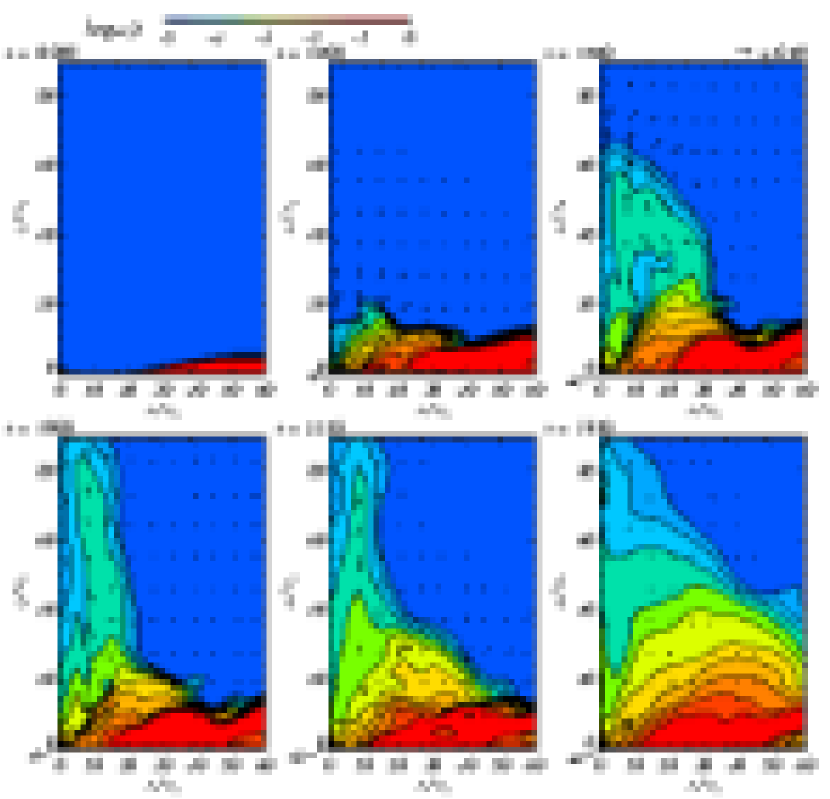
Figure 1.— Time evolution of the density contours of Model A with velocity vectors being overlaid. The density contours with colors are equally distributed on logarithmic scale with spacing being 0.4. The elapsed times are indicated in the upper-left corner of each panel. The unit of time is $r_{\rm s}/c=10^{-4}(M/10M_{\odot})$ s. A magnetic jet first grows at $t=1000\sim 1800$ but loses power at later times, producing more spherical density distribution.

We can roughly divide the entire evolution of a rotating torus initially threaded by poloidal fields into two distinct phases: a transient, extended jet phase (hereafter, Phase I) and a subsequent quasi-steady phase (or Phase II).

Figure 2 displays more detailed structure in Phase I of Model A. The left panel shows the contours of the plasma-$\beta$ on the logarithmic scale. We can easily distinguish jet regions which have blue colors and thus are in low-$\beta$, and ambient red regions which are in high-$\beta$. Most of matter inside the jet is blown outward, although downward motion is also observed partly, especially near the rotation axis. Total pressure (a sum of gas pressure and magnetic pressure) decreases with an increase of height in nearly plane-parallel fashion, as is shown by the contours by black solid lines. It is interesting to note that total pressure inside the jet is nearly uniform in the horizontal direction at $z>20$, indicating that the magnetic tower is balanced with the ambient gas pressure. Without external pressure by background corona, a magnetic tower would expand along the directions of 60^∘ tilted from the rotation axis (Lynden-Bell & Boily 1994). Model A shows that a magnetic tower evolves nearly in the vertical direction, which is made possible because of substantial external pressure (Lynden-Bell 1996).

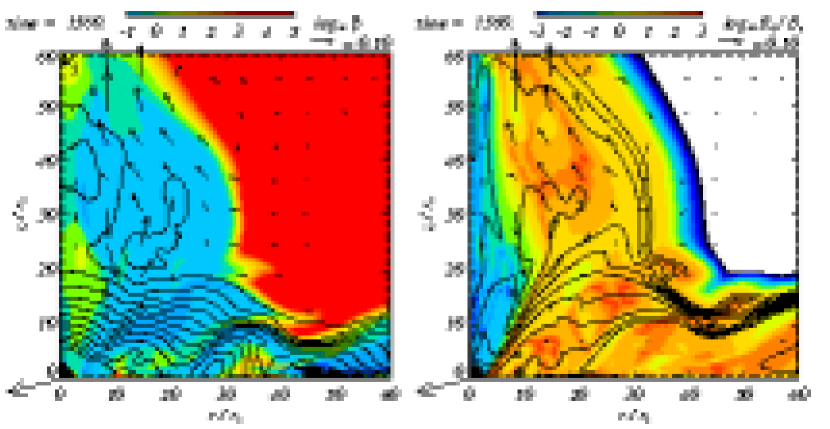
Figure 2.— Color contours of plasma-$\beta$ (left) and magnetic pitch (right) in Phase I of Model A, respectively, overlaid with velocity vectors and total pressure (left) and density (right) contours with black solid lines in logarithmic scale. Contour level of total pressure is $P_{tot}(N)=-6.0+0.15N$ where $N$ is integer from 0 to $14$ while that of density is same as fig 1.

The right panel of figure 2 shows the contours of the $B_{\rm\phi}/B_{\rm p}$. This figure is useful to check which of toroidal or poloidal fields are dominant in which region. We can immediately understand that the core of the jet has a blue color, implying poloidal components being more important, while the surrounding zone of the jet has a orange color, indicating dominant toroidal field components. Obviously, toroidal fields can be easily generated, as matter drifts inward, owing to faster rotation and larger shear at smaller radii.

Such different field configurations near the surface and in the core of the jet is more artistically visualized in the three-dimensional fashion in figure 3. Here, thick red lines indicate magnetic field lines and thick green-to-blue lines represent streamlines with indication of velocities by the color; the blue, green, and yellow represent velocities of $\sim 0.1$, 0.3, and 0.4 (in the unit of $c$), respectively. We can understand why magnetic field configuration of a sort that we encounter here is called as “a magnetic tower.” Volume inside the tower is mostly occupied by tightly wound toroidal fields. At the same time, we also observe vertical field lines in the core of the jet. As time goes on, this magnetic tower inflates vertically due to the growing magnetic pressure by the accumulated toroidal fields. Accordingly, the jet is also driven by enhanced magnetic pressure of the magnetic tower. Matter attains velocity up to $\sim 0.1-0.2c$ at the top.

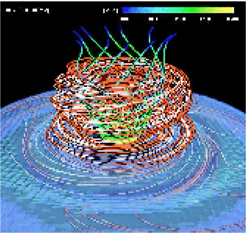
Figure 3.— Perspective view of magnetic fields lines in Phase I of Model A. Thick red (or thin white) lines indicate magnetic field lines which are anchored to the innermost (somewhat outer) zones at $(r,z)=(1,1.5)$ [$(r,z)=(56,10)$], respectively. Thick green lines denote the streamlines of velocity vectors integrated from $(r,z)=(8.5,7)$, whereas the color bar indicate the velocity. Light-blue shaded region indicate the isovolume of the density ($\rho=0.025\rho_{0}$). Accumulated toroidal fields emerging from the disk produce a magnetic tower, thereby driving an MHD jet. Jet material is surrounded by toroidal magnetic fields, whereas poloidal (vertical) fields dominate inside the jet.

We have checked how much fraction of energy leaves the calculation box in which form (see Table 3). The values in the table are shown by the percentage of the sum of time-averaged fluxes listed in the column at each phase. Generally, the energy carried by jets does not dominate the total energy loss from the system. In Model A, for example, the outflow energy is only $\sim 0.5\%$ of the total energy loss.

Table 3Fraction of flux.

flow	flux	A/I [%]	A/II [%]	B [%]	C [%]	D [%]
outflow	$c\langle\mbox{\boldmath$E$}\times\mbox{\boldmath$B$}\rangle_{z}\tablenotemark{\textdaggerdbl}~{}/4\pi$	$0.13$	$0.00$	$0.00$	$3.14$	$0.53$
	$\langle(\rho v^{2}/2)\mbox{\boldmath$v$}_{z}\rangle$	$0.14$	$0.00$	$0.00$	$8.99$	$0.69$
	$\langle\gamma p/(\gamma-1)\mbox{\boldmath$v$}_{z}\rangle$	$0.27$	$0.00$	$0.00$	$1.21$	$0.21$
inflow	$c\langle\mbox{\boldmath$E$}\times\mbox{\boldmath$B$}\rangle_{in}\tablenotemark{*}~{}/4\pi$	$0.03$	$0.03$	$0.05$	$1.0$	$0.22$
	$\langle(\rho v^{2}/2)\mbox{\boldmath$v$}_{in}\rangle$	$29.11$	$29.25$	$28.34$	$28.29$	$28.19$
	$\langle\gamma p/(\gamma-1)\mbox{\boldmath$v$}_{in}\rangle$	$30.99$	$31.13$	$30.15$	$34.94$	$30.20$
	$\langle\rho\psi\mbox{\boldmath$v$}_{in}\rangle$	$39.42$	$39.60$	$41.45$	$24.96$	$40.40$

3.2. Quasi-steady MHD flow

Eventually the initial jet loses its power, and the system enters a quiet, quasi-steady state. First, we show in figure 4 the radial distributions of representative physical quantities in both of Phase I (by the thick solid lines) and Phase II (by the thick dashed lines). The adopted quantities are density, radial velocity, pressure, specific angular momentum, sound velocity, and mass accretion rate, $\dot{M}\equiv-\int_{0}^{H}2\pi r\rho v_{r}dz$ with $H=1.0$ being fixed. These quantities are azimuthally and vertically averaged over $0\leq\phi\leq 2\pi$, $0\leq z\leq 1$ except the mass accretion rate which is a vertical integral.

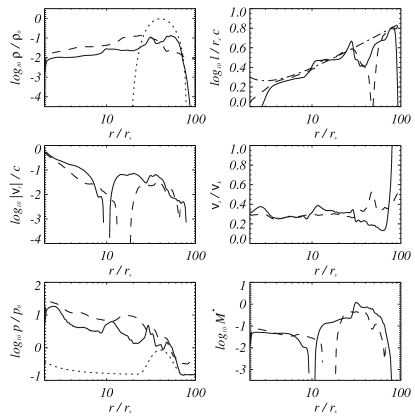
Figure 4.— Radial structure of the flow of Model A on the equatorial plane in Phase I ($t=1560\;r_{\rm s}/c$; transient extended jet phase) by the solid curves and in phase II ($t=3910\;r_{\rm s}/c$; subsequent quasi-steady phase) by the dashed curves, respectively. From the top left to the right bottom, density, radial velocity, pressure, specific angular momentum, sound velocity, and mass accretion rate are plotted. The dotted lines indicate initial conditions for density and pressure, while a dash-dotted line indicates a Keplerian specific angular momentum.

Roughly speaking, these quantities show power-law relations; i.e., $\rho\propto r$ at small radii, while $\rho\propto r^{-1}$ at large radii, $v_{r}\propto r^{-1/2}$ except at the inner outflowing part, $\ell$ (specific angular momentum) $\propto r^{0.5}$, meaning a nearly Keplerian rotation, $c_{\rm s}$ (sound velocity) $\propto r^{-1/2}$, and $\dot{M}\sim$const. in space in the inner region. All of these relations resemble closely those of the previous work (i.e., Stone & Pringle 2001, HB02). Note that our results are consistent with a hot, thick, near-Keplerian disk, and a subthermal magnetic field. The density distribution is inconsistent with ADAF models, since ADAF shows a steeper density profile, approximately $\rho\propto r^{-3/2}$.

The most interesting feature in the present simulations is found in figure 5, which illustrates contours of the total pressure (by black solid lines) and plasma-$\beta$ (by color contours) in the left panel and those of density (by black solid lines) and $B_{\phi}/B_{p}$ (by color contours) in the right panel in Phase II of Model A calculations. We find that total pressure distribution is not plane-parallel and the plasma-$\beta$ distribution has inhomogeneous structure around the central black hole.

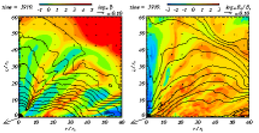
Figure 5.— Same as Fig. 2 but in Phase II of Model A.

Interestingly, high-$\beta$ ($\sim 100$) plasmas (indicated by orange color in the left panel) distributed in the radially extended zone which is tilted by $\sim 30^{\circ}$ from the $z$-axis (in the perpendicular direction to the iso-pressure contours) are sandwiched by moderately low-$\beta$ ($<1$) plasmas indicated by blue color. There is another high-$\beta$ region extending from point ($r,z$)$\sim$($15,0$) to the upper left region. We also notice that poloidal (or toroidal) fields are dominant in these high-$\beta$ (low-$\beta$) regions, as is indicated by orange (green or blue) colors in the right panel. As a consequence, mass accretion onto the central black hole takes place mainly through the equatorial plane at $r<20$. We also notice that poloidal (vertical) fields are still evident along the rotation axis, along which downward motion of gas is observed.

We find that equi-$\beta$ contours slightly change with time. The accretion flow is inherently time dependent, as it is driven by MHD turbulence. There are two possibilities for the origin of time dependence in this case. One is the axisymmetric mode of MRI (so-called channeling mode). Since the structure of quasi-steady flow is nearly-axisymmetric, the channeling mode of MRI can grow in our simulations. As a result, high-$\beta$ plasma is created between the low-$\beta$ plasmas with opposite directions of the flow. Another possibility is magnetic buoyancy. If we assume pressure balance among neighboring high- and low-$\beta$ regions, matter density should be high in the former, since magnetic pressure is less in the former. This gives rise to magnetic buoyancy for the latter, inducing its rising motion in the direction opposite to that of gravity. Such a rising magnetic loop was simulated by Turner, Bodenheimer, and Różyczka (1999), who found that the rising loop evolves into a jet (see also KMS02 for global simulations). In both cases, magnetic reconnection can be triggered. We find that the directions of toroidal fields are anti-parallel across high-$\beta$ region. Thus, magnetic reconnection can take place in this high-$\beta$ region and high-velocity plasmoid can be ejected from this site. If this is the case, high-$\beta$ region may move outward. Velocity vectors plotted in this figure show both of outward and inward motions, although their absolute values are small. The situation is rather complex. To make clear what is happening in the quasi-steady state, we need more careful studies.

It will be highly curious to see how magnetic field configuration changes after the jet eruptions. In figure 6 we plot the perspective view of the magnetic fields lines and matter trajectories in Phase II of Model A. Field line configurations are distinct from those in Phase I. Field lines which are connected to the innermost part of the flow (indicated by red thick lines) now show much simpler structure than in Phase I and are dominated by poloidal component, implying that toroidal fields found in Phase I have already been blown away. Note, however, that the surrounding region is still dominated by toroidal fields, as are indicated by white thick lines. As a consequence, the magnetic tower is not clearly seen.

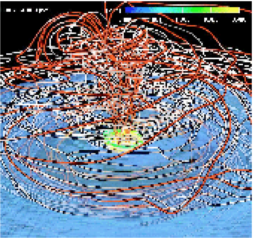
Figure 6.— Same as Fig. 3 but in Phase II of Model A. Magnetic fields lines represented by thick red lines are more confined, compared with those in figure 3. Thin white lines (representing the fields lines emerging from somewhat outer zones) look similar to those in figure 3. Thick green lines indicating the streamlines of velocity vectors only appear near the black hole and are not evident.

In order to see more clearly how toroidal and poloidal fields are generated and accumulated with time in the disk and the corona, we plot the strength of each component as a function of radius at several time steps in figure 7. Toroidal fields increase in strength by the shear and dominates in the entire region (at $t=1200$), but they are blown away from the disk by the emergence of a jet and thus decrease in strengths (at $t=1560$), whereas poloidal fields are generated due to the emergence of the magnetic tower from the disk. After the substantial ejection of matter and toroidal fields, the axial part of the corona $r<7$ is dominated by poloidal fields. Toroidal fields can be blown off with jet material, but poloidal fields created by vertical inflation of toroidal fields should remain. Note that, since no continuous injection of mass and fields are assumed in our calculation, the increase of the poloidal fields in the inner zone is eventually saturated. If we would add more fields, they would continuously grow.

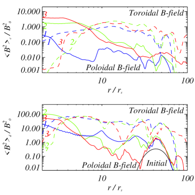
Figure 7.— Changes of the magnetic energy density in the disk (bottom panel) and in the corona (upper panel) from their initial values as functions of radius for Model A. Each panel presents the magnetic energy density of poloidal (solid lines) and that of toroidal fields (dashed lines). The magnetic energy in the disk (or in the corona) is integrated from $z=0$ to $z=5$ (from $z=5$ to $z=100$). The elapsed times are $1200$, $1560$, and $3910$ (in $r_{s}/c$), corresponding to the labels 1, 2, and 3, respectively.

We finally plot the energetics of Model A in figure 8. Kinetic energy always dominate others in both phases. That is, magnetic fields are not strong enough to suppress accreting motion of the gas. There is no evidence of huge buildup of net field which would inhibit accretion onto the central black hole in our simulations, unlike the picture obtained by INA03.

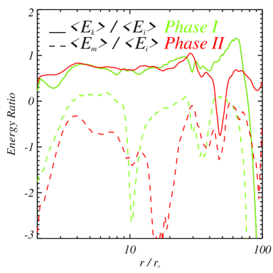
Figure 8.— Energetics of Model A. The ratio of kinetic energy ($E_{\rm k}$) to thermal energy ($E_{\rm i}$) and the ratio of magnetic energy ($E_{\rm mag}$) to thermal energy ($E_{\rm i}$) are plotted as functions of radius in Phases I ($t=1560\;r_{\rm s}/c$) and II ($t=3910\;r_{\rm s}/c$), respectively. Kinetic energy always dominate over others by about one order of magnitude.

3.3. Cases of weak initial fields and/or low external pressure

Before closing this section, let us see some parameter dependence of our results. In Models B – D, we vary the initial magnetic-fields strengths and/or external pressure by background corona. To help understanding different conditions, we plot the initial radial distribution of pressure (gas and magnetic) in figure 9 for each model. We see that external pressure is comparable to initial torus pressure in Models A and B, while the external pressure is totally negligible in Models C and D.

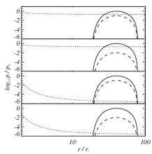
Figure 9.— Initial pressure distributions for Model A, B, C, and D from the top. The solid and dashed lines represent the gas and magnetic pressures at $z=0$, respectively, where as the dotted lines represent external pressures by background corona extrapolated to the $r$-axis ($z=0$; see equation 10). All values are normalized by the pressure at the density maximum of the torus ($r$, $z$)=($r_{0}$,0)

The later evolution is shown in figure 10. First, the case of initially weaker magnetic fields (Model B) is displayed in the second row of figure 10. Importantly, we do not see a strong outflow. The absence of an obvious jet can be understood in terms of pressure balance. Since magnetic field strength is by one order of magnitude smaller in Model B than that in Model A, the initial magnetic pressure is much smaller than external pressure (see figure 9). Magnetic pressure can grow as disk dynamo works, but magnetic pressure is not yet large enough to overcome external pressure at the moment that the disk material reaches the innermost region. Note that the time needed for the torus material reaches the center is much longer in Model B than in Model A, because it takes a longer time for fields to be strong enough to promote rapid accretion. Since the magnetic pressure inside the disk is comparable to the background pressure in Model A initially, it is easy to overcome the background pressure. Hence, eruption of a magnetic jet is possible. Nevertheless, it is interesting to note that the subsequent states look similar among Models A and B. This indicates that Phase II structure is not sensitive to the strengths of initial magnetic fields, although it is not yet clear that the results may or may not depend on the initial magnetic field orientations.

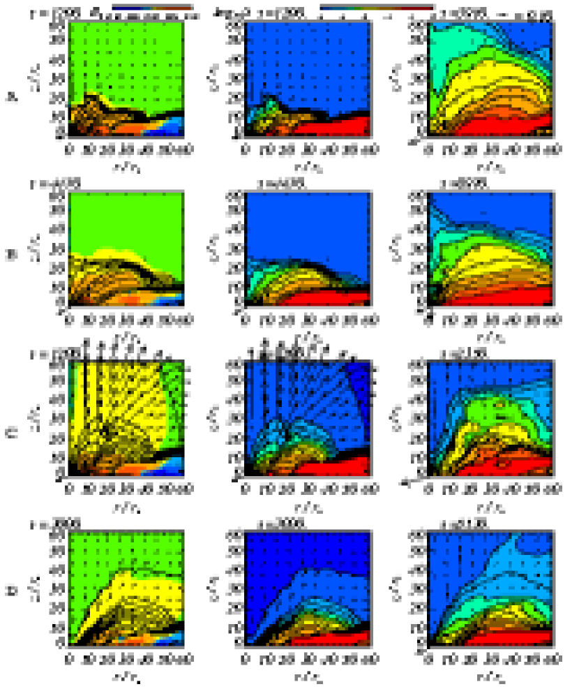
Figure 10.— Summary of the results of 4 calculated models. From the left to the right, contours of toroidal field strengths and of density in different time are displayed for Models A, B, C, and D from the top. Arrows show the velocity vectors. Initial magnetic fields strengths are weaker in Models B and D (in which $\beta=100$ while $\beta=10$ otherwise), while external pressure is 10 time weaker in Models C and D.

The cases of weaker external pressure (Models C and D) are illustrated in the third and fourth rows of figure 10. We find stronger, wider, and longer-standing (nearly persistent) jet in these models. This demonstrates that duration of a jet, as well as its width, are sensitive to how large external pressure is. Again, the flow structure in Phase II looks similar among Models C and D, but unlike cases with stronger external pressure (Models A and B) there is a conical low-density region present near the symmetric ($z$-) axis. This is due to the ejection of mass from the innermost part via jets.

We find in table 3 that the total energy output by the jet amount to $\sim 10$% of the total energy loss at maximum in Model C (with strong initial magnetic field and low external pressure). Except this model, total energy output is negligible. How much fraction of energy can be carried away from the black hole system thus depends critically on external pressure and field strength, and it is not always possible to achieve a high efficiency of energy extraction by jets.

Finally, we summarize our simulation results in the schematic picture (see figure 11). In figure 11, high-$\beta$ plasma with highly turbulent motion locates at the equatorial plane. Magnetic field generated by the dynamo action taking place inside the disk emerges upward and create the disk corona with intermediate-$\beta$ plasma. In the inner region of the disk, the emerging magnetic field erupts into the external corona and deform into the shape of the magnetic tower. Such magnetic tower ejects disk materials upward by its magnetic pressure and creates the magnetic tower jet. The magnetic tower jet collimates at the radius where the magnetic pressure of the tower is balanced with the external pressure.

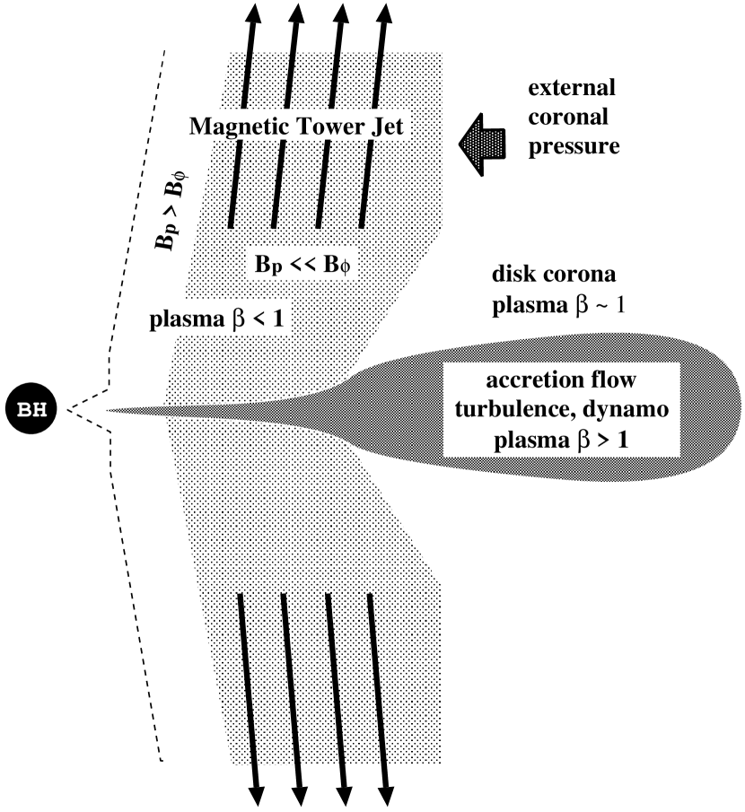
Figure 11.— Schematics of the magnetic tower jets.

4. DISCUSSION

4.1. Brief Summary

We performed 3-D MHD simulations of the radiatively inefficient rotating accretion flow around black holes. We examined the case with initially poloidal field configurations with $\beta=10$ and 100. When the bulk of torus material reaches the innermost region close to the central black hole, a magnetic jet is driven by magnetic pressure asserted by accumulated toroidal fields (magnetic tower). The fields are mostly toroidal in the surface regions of the jets, whereas poloidal (vertical) fields dominate in the inner core of the jet. The collimation width of the magnetic jet depends on external pressure; the more enhanced the external pressure is, the more collimated the jet is. Non-negligible external pressure tends to suppress the emergence of the MHD jets.

The jet outflow is, however, a transient phenomenon, unless the external pressure is negligible. After several dynamical timescales at the radius of the initial torus, the jet region shrinks and the flow structure completely changes. After the change, the flow is quasi-steady and possesses complex field configurations.

The nature of the quasi-steady state differs from that of INA03. We have seen that poloidal fields are dominant near the $z$-axis and that the black hole is mostly surrounded by marginally low-$\beta$ plasma with toroidal fields being dominant. This view is different from that simulated by INA03, who found a magnetosphere composed of a significantly low-$\beta$ ($\sim 10^{-3}$) plasmas with poloidal fields and that mass is not allowed to directly pass into the magnetosphere. Instead, mass accretion occurs along the radial narrow streams with slow rotation. We will discuss in §4.3 what the origin of difference would be.

4.2. Magnetic Tower Jet

The acceleration mechanism of the MHD jet, starting with a disk threaded with large-scale, external vertical fields, has been studied extensively by many groups. It has been discussed that in the magneto-centrifugally driven jet, the poloidal magnetic field is much stronger than the toroidal magnetic field in the surface layer of the disk or in the disk corona, where plasma-$\beta$ is low (e.g., Blandford and Payne 1982; Pudritz and Norman 1986; Lovelace et al. 1987). In this case, magnetized plasma corotates with the disk until the Alfvén point, beyond which toroidal field starts to be dominated and hence collimation begins by its magnetic pinch effect. Blandford-Payne (1982) mechanism can be applied to this kind of jet for determining the launching point of the jet.

On the other hand, there is another kind of magnetically driven jet, in which the toroidal magnetic field is dominated everywhere (e.g., Shibata and Uchida 1985; Shibata, Tajima, Matsumoto 1990; Fukue 1990; Fukue, Shibata, Okada 1991; Contopoulos 1995). In this case, Alfvén point is embedded in the disk or there is no Alfvén point, and the collimation due to toroidal field begins from the starting point of the jet. Blandford-Payne mechanism cannot be applied to such jet.

Situation is similar, if magnetic loops are anchored to the surface of the differentially rotating disk or that of the central object. MHD jet generated from the weak, localized poloidal field in the disk (Turner et al. 1999, KMS02) belong to the toroidal field dominated jet. Moreover, MHD jet generated from the dipole magnetic field is simulated by Kato, Hayashi, & Matsumoto (2004). They calculated time evolution of a magnetic tower jet, which is an extension of Lynden-Bell (1996)’s magnetic tower, and is also the toroidal field dominated jet.

Our magnetic tower jet is also consistent to the toroidal field dominated jet, since the magnetic tower is made of the toroidal field generated by dynamo action within the disk. It has often been argued that such a toroidal field dominated jet is very unstable for kink instability in real 3D space, and cannot survive in actual situation (e.g., Spruit, Foglizzo, Stehle 1997). However, our 3D simulations showed, for the first time, that such toroidal field dominated jet survive at least for a few orbital periods of the disk and hence can be one of promising models for astrophysical jets.

By means of the magnetic tower jets, one may ask what the condition for the formation of the toroidal field dominated jet is. The formation of magnetic jets demand that the maximum magnetic pressure $p_{\rm mag}^{\rm max}$ generated within the disk must exceed the external pressure $p_{\rm ext}$. Since the growth of toroidal fields due to MRI is saturated under a certain value (e.g., $\beta_{min}\sim 100$ within the disk; see Matsumoto et al. 1999; Hawley 2000; INA03), we have a condition for the formation of the jet as follows:

$$p_{\rm mag}^{max}=p_{\rm disk}/\beta_{min}>p_{\rm ext},$$ (13)

where $p_{\rm disk}$ is the pressure of the disk. Our conclusion is equivalent to that of KMS02 for the case of isothermal background corona, in which they argued that if the coronal density is very high, it prevents the ejection of magnetic loop.

If external pressure is very small, compared with initial torus (magnetic) pressure, magnetic fields can more easily escape from the disk than otherwise. The result is a strong, long-persistent jet, as we saw in Models C and D. Although the collimation is not clear in the plot with limited box, collimation does occur but at large radii ($>60r_{s}$) in these models, since, as the outflow expands magnetic pressure decreases and eventually becomes comparable to the external pressure. We thus call it a jet, not a big wind, and the width of the jet depends on the external pressure.

If external pressure is very large and by far exceeds the maximum magnetic pressure inside the disk, conversely, the emergence of magnetic fields out of a disk is totally inhibited, the situation corresponding to Model B. There will be no jets. Only when external pressure is mildly strong, comparable to the maximum magnetic pressure, we can have a transient eruption of a collimated magnetic jet (see Model A).

It is important to note, in this respect, the works by Lynden-Bell. Lynden-Bell & Boily (1994) studied self-similar solutions of force-free helical field configurations, finding that such configurations expand along a direction of 60 degrees away from the axis of helical field. Modified model by Lynden-Bell (1996) asserts that a magnetic tower can be confined by external pressure. Here, by 3-D MHD simulation, we successfully show that the formation process of magnetic tower, which is stable for a few dynamical timescale at the density maximum of the initial torus. Our 3-D magnetic tower solution is basically the same as that he proposed.

Unfortunately, there were not always detailed descriptions regarding external pressure given in previous MHD simulation papers, although the presence of external pressure is indispensable to perform long-term simulations. INA03 claimed that even with continuous supply of mass and fields, bipolar jet (or outflow) phase is transient. Their case seems to correspond to the case with relatively strong external pressure (i.e., our Model A). If this is the case in actual situations, we expect strong jets only when a burst of large accretion flow takes place. This may account for the observations of a micro-quasar, GRS1915+105, which recorded big (superluminal) jets always after sudden brightening of the system (Klein-Wolt et al. 2002).

It is interesting to discuss the collimation mechanisms of the jet. We checked the force balance, confirming that it is external pressure that is balanced with magnetic pressure at the boundary between the jet and the ambient corona. Together with our finding that jet widths depend also on the value of external pressure, we are led to conclusion that for jet collimation, external pressure play important roles in the present case.

Furthermore, the total pressure of magnetically dominated “corona”, created above the disk due to the eruption of the magnetic tower jet in early phase, could be greater than that of the background pressure (hereafter we call it as “disk corona” in order to distinguish from background corona; see also two-layered structure of accretion flow as presented by HB02). Thus we expect that the collimation widths of a successive jet would be smaller than that in the case of Model A.

To sum up, we demonstrate the important role of external pressure asserted by ambient coronal regions on the emergence, evolution, and structure of a magnetically driven jet. We need to remark how feasible the existence of a non-negligible external pressure is in realistic situations. Fortunately, we have a good reason to believe that ambient space of accretion flow system may not be empty. If there is magnetic dynamo activity in the flow, magnetic fields will be amplified and eventually escape from the flow forming a magnetically confined corona (Galeev, Rosner, & Vaiana 1979). Then, mass can be supplied from the flow to a corona via conduction heating of the flow material. In fact, the density of the disk corona is basically explained by the energy balance between conduction heating and evaporation cooling of disk chromosphere (Liu, Mineshige, & Shibata 2002). Thus, it is reasonable to assume that ambient space surrounding a magnetized flow is full with hot tenuous plasmas as a result of previous magnetic activity of the disk and that the hot corona exerting external pressure on the flow with comparable magnitude.

Finally, we remark on the comparison with the simulations by HB02. They also calculated the evolution of a torus threaded with poloidal fields, adopting similar initial conditions as we did. But there is a distinction; we find a significantly low-$\beta$ jet, whereas HB02 obtained a high-$\beta$ jet (see their figure 1).

In contrast to HB02, our jet is driven by the magnetic pressure inside magnetic tower. Although we found the outflow along the funnel barrier inside the core of magnetic tower in Model C and D (fig 10), the outflow is not driven by the gas pressure but the magnetic pressure. Furthermore, we note that averaged plasma-$\beta$ along the funnel barrier where the poloidal field dominates the toroidal field is of the order of unity (fig 5). In comparison with HB02, the discrepancy can be explained by the difference of external pressure. For instance, in Model C and D, there are persistent jets which look like uncollimated winds reported in HB02. This is because that the external pressure was too low to confine the magnetic tower inside the computational box.

4.3. Steady-State Picture of MHD Accretion Flow

The flow structures in the quasi-steady phase which we obtained in our simulations look similar to that of previous work except INA03. There is a big distinction; INA03 claimed the formation of a significantly low-$\beta$ (with $\beta\sim 10^{-3}$) magnetosphere dominated by a dipolar magnetic field. Since any motion passing through the magnetosphere is inhibited, accretion occurs mainly via narrow slowly-rotating radial streams. We, in contrast, find the formation of a $\beta\sim 1$ region (on average) which is dominated by toroidal magnetic fields, although the structure is quite inhomogeneous and is a mixture of high- and low-$\beta$ zones. Importantly, the fields are not too strong to inhibit gas accretion, since magnetic field strength is amplified by the dynamo action inside the disk due to MRI and the spatially averaged plasma-$\beta$ inside the disk is unlikely to become less than unity in general. Mass accretion occurs predominantly along the equatorial plane. Mass inflow toward the black hole from the other directions is also found, but mass flow rates are not large because of smaller density than the value on the equatorial plane.

We can easily demonstrate that it is not easy to create an extended magnetosphere which has significantly low-$\beta$ values. Suppose that magnetic fields are completely frozen into material. As a gas cloud contracts, it gets compressed due to geometrical focusing. If the gas cloud shrinks in nearly a spherically symmetric way, the density and gas pressure increases as $\rho\propto r^{-3}$ and $p\propto\rho^{\gamma}\propto r^{-5}$ for $\gamma=5/3$, respectively, in radiatively inefficient regimes. Because of the frozen-in condition, poloidal fields are also amplified according to the relation, $B_{z}\propto r^{-2}$, as long as the total magnetic flux, $B_{z}r^{2}$, is conserved. That is, magnetic pressure also increases but more slowly, $p_{\rm mag}>{B_{z}}^{2}/8\pi\propto r^{-4}$. Thus, the plasma-$\beta$ should $increase$ as gas cloud contracts, as $\beta\equiv p_{\rm gas}/p_{\rm mag}\propto r^{-1}$. Regions just above and below the black hole (in the vertical direction) can have low-$\beta$ plasmas, since matter can slide down to the black hole along the vertical fields, but it is unlikely that low-$\beta$ regions can occupy a large volume.

If gas cloud shrinks in the two-dimensional fashion, conversely, the plasma-$\beta$ will decrease as gas cloud contract, since then gas density is proportional to $\rho\propto r^{-2}$, thus yielding $p_{\rm gas}\propto r^{-2\gamma}\propto r^{-10/3}$ (for $\gamma=5/3$) and $\beta\propto r^{2/3}$. This is not the case in our simulations, which show that matter is more concentrated around the equatorial plane.

It might be noted that the surface of a magnetosphere may be unstable against the magnetic buoyancy instabilities such as interchange instability (so-called magnetic Rayleigh-Tayer instability; Kruskal & Schwarzschild 1954) and undular instability (so-called Parker instability; Parker 1966), since heavy materials are located above field lines with respect to the direction of gravity. Roughly speaking, the critical wavelength, over which perturbation is unstable against the Parker instability, is $\lambda_{\rm c}\sim 4\beta^{-1/2}H$ (with $H$ being the pressure scale-height; see Matsumoto et al. 1988). When $\beta\sim 10^{-3}$, we have $\lambda_{\rm c}\sim 100H>r$, since $H/r$ cannot be as small as $H/r\sim 10^{-2}$. The Parker instability is completely stabilized under such circumstances but interchange instability can occur (e.g., Wang & Nepvue 1983). In our case with a relatively large $\beta\sim 1$, on the other hand, there are frequent chances to trigger the Parker instability. The growth time scale of the Parker instability is $(2-4)H/v_{\rm A}$. As a result, heavy gas easily sink down through a moderately magnetized region.

We need to note again that kinetic energy (including orbital energy) always dominate over magnetic and thermal energy, meaning that there is no sign of huge magnetic fields inhibiting accretion as INA03 claimed. It is not clear if magnetic buoyancy instability helps accreting motion of gas. Further, we should note that anomalous resistivity always turns on near the black hole, meaning the effective occurrence of magnetic reconnection. In any cases, our picture of the quasi-steady phase of MHD accretion flow is that matter can accrete onto a black hole on relatively short timescale.

We studied the case of initially poloidal fields. A natural question is how universal our conclusion is. The simulations starting with toroidal fields (INA03; Machida & Matsumoto 2003) show no strong indication of magnetic jets. This is a big difference. However, toroidal fields can be more easily created by differential rotation than poloidal fields. We thus find that toroidal fields can suddenly grow and dominate over poloidal fields in a large volume (see figure 7). We can expect similar quasi-steady state, even if we start calculations with toroidal fields. To this extent, our study is consistent with those of initially toroidal field with the low external pressure. The comparison is left as future work.

References

- Abramowicz, Czerny, Lasota, & Szuszkiewicz (1988) Abramowicz, M. A., Czerny, B., Lasota, J. P., & Szuszkiewicz, E. 1988, ApJ, 332, 646
- Balbus (2003) Balbus, S. A. 2003, ARA&A, 41, 555
- Balbus & Hawley (1991) Balbus, S. A. & Hawley, J. F. 1991 ApJ, 376, 214
- Blandford & Begelman (1999) Blandford, R. D. & Begelman, M. C. 1999, MNRAS, 303, L1
- Blandford & Payne (1982) Blandford, R. D. & Payne, D. G. 1982, MNRAS, 199, 883
- Casse & Keppens (2002) Casse, F. & Keppens, R. 2002, ApJ, 581, 988
- Contopoulos (1995) Contopoulos, J. 1995, ApJ, 450, 616
- Ebisawa (1999) Ebisawa, K. 1999, in High Energy Processes in Accreting Black Holes (ASP Conf. Ser. 161), ed. J. Poutanen & R. Svensson, p.39
- Fukue (1990) Fukue, J. 1990, PASJ, 42, 793
- Fukue, Shibata, & Okada (1991) Fukue, J., Shibata, K., & Okada, R. 1991, PASJ, 43, 131
- Galeev, Rosner, & Vaiana (1979) Galeev, A. A., Rosner, R., & Vaiana, G. S. 1979, ApJ, 229, 318
- Hawley (2000) Hawley, J. F. 2000, ApJ, 528, 462
- Hawley (2001) Hawley, J. F. 2001, ApJ, 554, 534
- Hawley & Balbus (2002) Hawley, J. F., & Balbus, S. A. 2002 ApJ, 573, 738 (HB02)
- Hawley, Balbus, Stone (2001) Hawley, J. F., Balbus, S. A. & Stone, J. M. 2001, ApJ, 554, L49
- Hawley & Krolik (2001) Hawley, J. F. & Krolik, J. H. 2001, ApJ, 548, 348
- Ichimaru (1977) Ichimaru, S. 1977, ApJ, 214, 840
- Igumenshchev, Abramowicz (2000) Igumenshchev, R., & Abramowicz, M.A. 2000, ApJS, 130, 463
- Igumenshchev, Abramowicz, Narayan (2000) Igumenshchev, R., Abramowicz, M.A., & Narayan, R. 2000, ApJ, 523, L27
- Igumenshchev, Narayan & Abramowicz (2003) Igumenshchev, I., Narayan, R., & Abramowicz, M. A. 2003, ApJ, in press (INA03)
- Kato, Fukue, & Mineshige (1998) Kato, S., Fukue, J., & Mineshige, S. 1998, Black-hole accretion disks. Edited by Shoji Kato, Jun Fukue, and Sin Mineshige. Publisher: Kyoto, Japan: Kyoto University Press, 1998. ISBN: 4876980535, Chap. 10
- Kato, Hayashi, Matsumoto (2004) Kato, Y., Hayashi, M. R. & Matsumoto, R. 2004, ApJ, in press
- Klein-Wolt et al. (2002) Klein-Wolt, M., Fender, R. P., Pooley, G. G., Belloni, T., Migliari, S., Morgan, E. H., & van der Klis, M. 2002, MNRAS, 331, 745
- Kruskal & Schwarzschild (1954) Kruskal, M., Schwarzschild, M. 1954, Proc. Roy. Soc. (London) A, 223, 348
- Kudoh, Matsumoto, & Shibata (1998) Kudoh, T., Matsumoto, R., & Shibata, K. 1998, ApJ, 508, 186
- Kudoh, Matsumoto, & Shibata (2002) Kudoh, T., Matsumoto, R., & Shibata, K. 2002, PASJ, 54, 267
- Liu, Mineshige, & Shibata (2002) Liu, B. F., Mineshige, S., & Shibata, K. 2002, ApJ, 572, L173
- Lovelace, Wang, & Sulkanen (1987) Lovelace, R. V. E., Wang, J. C. L., & Sulkanen, M. E. 1987, ApJ, 315, 504
- Lynden-Bell (1996) Lynden-Bell, D. 1996, MNRAS, 279, 389
- Lynden-Bell & Boily (1994) Lynden-Bell, D., & Boily, C. 1994, MNRAS, 267, 146
- Machida, Hayashi, & Matsumoto (2000) Machida, M., Hayashi, M. R., & Matsumoto, R. 2000, ApJ, 532, L67
- Machida & Matsumoto (2003) Machida, M. & Matsumoto, R. 2003, ApJ, 585, 429
- Machida, Matsumoto, & Mineshige (2001) Machida, M., Matsumoto, R., & Mineshige, S. 2001, PASJ, 53, L1
- Matsumoto (1999) Matsumoto, R. 1999, in Numerical Astrophysics, ed. S. M. Miyama, K. Tomisaka, & T. Hanawa (Boston, Kluwer Academic), p.195
- Matsumoto et al. (1988) Matsumoto, R., Horiuchi, T., Shibata, K., & Hanawa, T. 1988, PASJ, 40, 171
- Matsumoto et al. (1996) Matsumoto, R., Uchida, Y., Hirose, S., Shibata, K., Hayashi, M. R., Ferrari, A., Bodo, G., & Norman, C. 1996, ApJ, 461, 115
- Mineshige, Kusnose, & Matsumoto (1995) Mineshige, S., Kusnose, M., & Matsumoto, R. 1995, ApJ, 445, L43
- Nakamura, Kusunose, Matsumoto, & Kato (1997) Nakamura, K. E., Kusunose, M., Matsumoto, R., & Kato, S. 1997, PASJ, 49, 503
- Narayan (2002) Narayan, R. 2002, in Lighthouses of the Universe, 2002, ed. M. Gilfanov, R. Sunyaev, & E. Churazov (Berlin, Springer), p.405
- Narayan & Yi (1994) Narayan, R. & Yi, I. 1994, ApJ, 428, L13
- Narayan & Yi (1995) Narayan, R. & Yi, I. 1995, ApJ, 452, 710
- Narayan, Mahadevan, & Quataert (1998) Narayan, R., Mahadevan, R., & Quataert, E. 1998, Theory of Black Hole Accretion Disks, 148
- Paczynsky & Wiita (1980) Paczyńsky, B. & Wiita, P. J. 1980, A&A, 88, 23
- Parker (1966) Parker, E. N. 1966, ApJ, 145, 811
- Pudritz & Norman (1986) Pudritz, R. E. & Norman, C. A. 1986, ApJ, 301, 571
- Quataert & Gruzinov (2000) Quataert, E. & Gruzinov, A. 2000, ApJ, 539, 809
- Richtmyer & Morton (1967) Richtmyer, R. D. & Morton, K. W. 1967, Interscience Tracts in Pure and Applied Mathematics, New York: Interscience, 1967, 2nd ed., chap. 13
- Rubin & Burstein (1967) Rubin, E.L. & Burstein, S.Z. 1967, J. Comp. Phys., 2, 178
- Shapiro, Lightman, & Eardley (1976) Shapiro, S. L., Lightman, A. P., & Eardley, D. M. 1976, ApJ, 204, 187
- Shibata & Uchida (1985) Shibata, K. & Uchida, Y. 1985, PASJ, 37, 31
- Shibata & Uchida (1986) Shibata, K. & Uchida, Y. 1986, PASJ, 38, 631
- Shibata, Tajima, & Matsumoto (1990) Shibata, K., Tajima, T., & Matsumoto, R. 1990, ApJ, 350, 295
- Spruit, Foglizzo, & Stehle (1997) Spruit, H. C., Foglizzo, T., & Stehle, R. 1997, MNRAS, 288, 333
- Stone & Pringle (2001) Stone, J. M. & Pringle, J. E. 2001, MNRAS, 322, 461
- Stone, Pringle, & Begelman (1999) Stone, J. M., Pringle, J. E., & Begelman, M. C. 1999, MNRAS, 310, 1002
- Turner, Bodenheimer, & Różyczka (1999) Turner, N. J., Bodenheimer, P., & Różyczka, M. 1999, ApJ, 524, 129
- Uchida & Shibata (1985) Uchida, Y. & Shibata, K. 1985, PASJ, 37, 515
- Wang & Nepveu (1983) Wang, Y.-M. & Nepveu, M. 1983, A&A, 118, 267
- Yokoyama & Shibata (1994) Yokoyama, T. & Shibata, K. 1994, ApJ, 436, L197