Constraints on the Inner Cluster Mass Profile and the Power Spectrum Normalization from Strong Lensing Statistics

Abstract

Strong gravitational lensing is a useful probe of both the intrinsic properties of the lenses and the cosmological parameters of the universe. The large number of model parameters and small sample of observed lens systems, however, have made it difficult to obtain useful constraints on more than a few parameters from lensing statistics. Here we examine how the recent WMAP measurements help improve the constraining power of statistics from the radio lensing survey JVAS/CLASS. We find that the absence of $\theta>3^{\prime\prime}$ lenses in CLASS places an upper bound of $\beta<1.25\,(1.60)$ at 68% (95%) CL on the inner density profile, $\rho\propto r^{-\beta}$, of cluster-sized halos. Furthermore, the favored power spectrum normalization is $\sigma_{8}\gtrsim 0.7$ (95% CL). We discuss two possibilities for stronger future constraints: a positive detection of at least one large-separation system, and next-generation radio surveys such as LOFAR.

1. Introduction

Strong gravitational lensing is a sensitive probe of the intrinsic properties of galaxies, clusters, and dark matter halos as well as of the underlying cosmological model of the universe. For instance, some of the earliest constraints on the cosmological constant were obtained from statistics of gravitational lensing (e.g. Turner 1990; Kochanek 1996). The uncertainties in the properties of the lenses themselves, however, have led some to suggest that lensing studies are better used as probes of lens properties rather than cosmological parameters (e.g. Cheng & Krauss 2000). This view is particularly pertinent in light of the recent measurements from the Wilkinson Microwave Anisotropy Probe (WMAP) and large-scale structure surveys, which, when combined, can now constrain some of the basic cosmological parameters to 5% or better (Spergel et al. 2003 and references therein).

Indeed, recent lensing studies have yielded useful constraints on the density profiles and velocity dispersions of galaxies (Takahashi & Chiba 2001; Rusin & Ma 2001; Oguri, Taruya & Suto 2001; Keeton & Madau 2001; Davis, Huterer & Krauss 2002; Chae 2002). Most of these analyses as well as direct observations (Cohn et al. 2001; Treu & Koopmans 2002; Winn, Rusin & Kochanek 2002; Rusin, Kochanek & Keeton 2003) indicate that the inner density profiles of elliptical galaxies are close to singular isothermal (SIS): $\rho\propto r^{-\beta}$ with $\beta\approx 2$. These analyses have been greatly facilitated by the completion of the Cosmic Lens All-sky Survey (CLASS; Myers et al. 2003, Browne et al. 2003), which extended the earlier Jodrell Bank-VLA Astrometric Survey (JVAS; King et al. 1999). JVAS/CLASS is the biggest survey with a homogeneous sample of lenses, with a total of about 16,000 sources and 22 confirmed lensing events. Among these, a subset of 8958 sources with 13 observed lenses forms a well-defined subsample suitable for statistical analysis (Browne et al. 2003, Table 13). In particular, the CLASS statistical subsample finds no lensing events with angular separations $\theta>3^{\prime\prime}$. An explicit search at $6^{\prime\prime}<\theta<15^{\prime\prime}$ also finds no lensing events (Phillips et al. 2002).

In this paper we study the constraints from strong lensing statistics in the post-WMAP era. We examine two of the currently most uncertain cosmological parameters: the equation of state of dark energy $w$ and the power spectrum normalization $\sigma_{8}$, as well as two of the most uncertain parameters in current lens models: the inner mass density profile of clusters $\beta$ and the mass scale $M_{c}$ that separates galaxy from cluster lenses. $N$-body simulations indicate that the dark matter profile in clusters has a roughly universal form with an inner logarithmic slope of $\beta\sim 1$ to 1.5 (Navarro, Frenk & White 1997; Moore et al 1999). However, recent analyses based on observations of arcs in clusters (e.g. Sand, Treu & Ellis 2002) indicate a shallower inner profile. This uncertainty has motivated us to treat $\beta$ for clusters as a free parameter in this study. For the galaxy-scale lenses with lower masses ($M<M_{c}$), we assume the SIS model in accordance with the results cited above. This two-population galaxy-cluster model is needed to account for the large number of observed small-separation lenses and the lack of $\theta>3^{\prime\prime}$ systems in JVAS/CLASS (Keeton 1998; Porciani & Madau 2000).

For the cosmological parameters, we use the results from WMAP in conjunction with ACBAR, CBI and 2dF experiments (Spergel et al. 2003). We use the mean values $n=0.97$, $\Omega_{M}h^{2}=0.134$ and $\Omega_{B}h^{2}=0.023$ (each measured to better than 5%), and marginalize over $\Omega_{M}=0.27\pm 0.04$ and $\sigma_{8}=0.84\pm 0.04$, although we find the strength of our final constraints on $\beta$ and $M_{c}$ to be insensitive to the strength of the particular priors used on $\Omega_{M}$ and $\sigma_{8}$. We consider only flat cosmological models.

2. Lens Profiles and Optical Depth

We write the total optical depth at a given lens mass as the sum of the optical depths due to SIS and generalized NFW (GNFW) halos:

$$\tau(M)=f_{SIS}(M)\tau_{\scriptscriptstyle SIS}(M)+(1-f_{SIS}(M))\tau_{\scriptscriptstyle GNFW}(M)$$ (1)

where $f_{SIS}$ is the fraction of halos that are SIS, and $1-f_{SIS}$ is the fraction that are GNFW. In addition to these two populations, there is some evidence that objects with $M\lesssim 10^{11}M_{\hbox{$\odot$}}$ have shallow profiles (Ma 2003, Li & Ostriker 2003). Ma (2003), for example, derives a form for $f_{SIS}$ by requiring the halo mass function and galaxy luminosity function to give consistent optical depth predictions at subsecond scale. Current lensing surveys are limited to $\theta\gtrsim 0.3^{\prime\prime}$, which cannot constrain small-mass halos. We therefore use the simplest possible form: $f_{SIS}=1$ for $M<M_{c}$ and 0 otherwise, and leave $M_{c}$ as a free parameter to be constrained by data.

An SIS lens has a density profile $\rho(r)=\sigma_{v}^{2}/(2\pi Gr^{2})$, where $\sigma_{v}$ is the 1-d velocity dispersion. SIS lenses produce an image separation of $2\theta_{E}$, where $\theta_{E}=4\pi(\sigma_{v}/c)^{2}D_{ls}/D_{s}$ is the Einstein radius, and the cross section is $\sigma_{\rm lens}=\pi(\theta_{E}D_{l})^{2}=16\pi^{3}(\sigma_{v}/c)^{4}(D_{l}D_{ls}/D_{s})^{2}$, where $D_{s},D_{l}$, and $D_{ls}$ are the angular diameter distances to the source, to the lens, and between the lens and the source, respectively. Using $\sigma_{v}=(\pi G^{3}M^{2}\Delta_{vir}\rho_{M}/6)^{1/6}$, we can then relate the cross-section $\sigma_{\rm lens}$ to the halo mass $M$ which is needed for eq. (1). The GNFW profile (Zhao 1996) is given by

$$\rho(r)={\rho_{s}\over\left(\displaystyle{r/r_{s}}\right)^{\beta}\left[1+\left(\displaystyle{r/r_{s}}\right)\right]^{3-\beta}}\,.$$ (2)

The mass of a halo is defined to be the virial mass $M=4\pi\Delta_{vir}\rho_{M}r^{3}_{vir}/3$, where $r_{vir}$ is the virial radius within which the average density is $\Delta_{vir}\rho_{M}$ and $\rho_{M}$ is the mean matter energy density in the universe. We compute $\Delta_{vir}$ from the spherical-collapse model using the fitting formula in Weinberg & Kamionkowski (2003). In practice, we replace the scale radius $r_{s}$ by a concentration parameter $c(z)\equiv r_{vir}(z)/r_{s}(z)$, which is well described (for $\beta=1$) by $c(z)=c_{0}(1+z)^{-1}(M/M_{*})^{-0.13}$ with $c_{0}=9$, where $M_{*}$ is a typical collapsing mass for that cosmology at redshift zero (e.g. Bullock et al. 2001). For $\beta\neq 1$, we compute $c_{0}$ by assuming that the ratio $r_{1/2}/r_{vir}$ is independent of $\beta$, where $r_{1/2}$ is the half-mass radius defined as $M(r<r_{1/2})=M(r<r_{vir})/2$ (Li and Ostriker 2002). The same redshift and mass dependence is used for all $\beta$.

The optical depth for lensing is given by (e.g., Turner, Ostriker & Gott 1984)

$$\tau=\int_{0}^{z_{s}}dz_{l}{dD_{l}\over dz_{l}}\,(1+z_{l})^{3}\int_{0}^{\infty}dM{dn\over dM}(M,z_{l})\,\sigma_{\rm lens}(M,z_{l})B$$ (3)

where $n(M,z_{l})$ is the physical number density of dark halos at the lens redshift $z_{l}$, $\sigma_{\rm lens}(M,z_{l})$ is the lensing cross section of a halo of mass $M$ at $z_{l}$, and $B$ is the magnification bias. We considered accounting for the ellipticity of lenses, but found that for the JVAS/CLASS luminosity function, ellipticity makes small ($\lesssim 10\%$) correction to the optical depth, and therefore we choose to ignore it. This is consistent with previous findings that ellipticity mostly affects image multiplicities (e.g. Kochanek & Blandford 1987; Wallington & Narayan 1993).

To model the number density of lenses, we use the halo mass function instead of the galaxy luminosity function (for the latter approach to constrain the dark energy equation of state, see Chae et al. 2002). The former has the advantages that (1) it accounts for all objects – dark and luminous – in the universe; (2) it has been accurately calibrated by $N$-body simulations; and (3) its main dependence is on now well-measured cosmological parameters instead of the more uncertain astrophysical parameters. We use the fitting formula of Jenkins et al. (2001) for $dn/dM$ but note that their halo mass is independent of cosmology and is defined to be the mass enclosed in radius $r_{vir}$ within which the average density is ($180\rho_{crit}$), instead of ($\Delta_{vir}\rho_{M}$) based on the spherical collapse model for general cosmology discussed earlier. We use the latter to define our halo mass in eq. (3), but for consistency, we convert it to $M_{180}$ and evaluate the fitting formula for $dn/dM$ at $M_{180}$. We find this step to lead to a relatively small upward correction to the optical depth. The matter power spectrum is an input to $dn/dM$; we use the formulae of Eisenstein & Hu (1997) for $w=-1$ models and those of Ma et al. (1999) for models with $w>-1$. We do not consider $w<-1$ since the power spectrum for these models is uncertain.

We include a scatter of $0.14$ in $\log_{10}c(z)$ (Bullock et al. 2001; note that the published version of this paper incorrectly quotes 0.18 for the scatter) for the halo concentration in eq. (3). We find that including this effect is very important, as it increases the GNFW optical depth by more than an order of magnitude, in rough agreement with Chen (2003) and Kuhlen, Keeton & Madau (2003).

To compute the magnification bias, we note that the sources in CLASS are well represented by a power-law luminosity function, $\phi(S)=dn/dS\propto S^{-\eta}$, with $\eta\simeq 2.1$, which leads to $B=4.76$ for all SIS lenses (Rusin & Tegmark 2001). The magnification bias is more complicated for GNFW lenses. We use the formula in Oguri et al. (2002), which agrees very well with ray-tracing simulations.

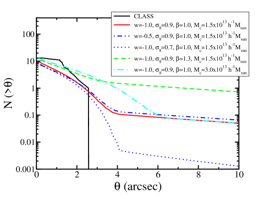
Figure 1.— Number of lenses with angular separation above $\theta$ from the CLASS statistical sample (Browne et al. 2003) and predictions from the compound lens model with different values of $w$, $\sigma_{8}$, $\beta$ and $M_{c}$. Halos with $M<M_{c}$ are assumed to have the SIS profile.

3. Results

Before discussing our statistical constraints on $\beta$, $M_{c}$, $\sigma_{8}$, and $w$, we first illustrate in Fig. 1 the dependence of lensing probability on these parameters by comparing the expected number of lenses $N(>\theta)$ in various models with the CLASS result. It shows that the value of $M_{c}$ and an upper limit on $\beta$ can be determined very accurately because the CLASS histogram has a sharp cut-off in $\theta$. Variations in $w$, on the other hand, have a fairly small effect at all scales. Models with low $\sigma_{8}$ underpredict the optical depth at $\theta\lesssim 3^{\prime\prime}$, while those with both high $\sigma_{8}$ and $\beta$ overpredict the optical depth for $\gtrsim 3^{\prime\prime}$. Finally, we find that $N(>\theta)$ is insensitive to the value of $\Omega_{M}$.

For the statistical tests, we use information from both the total lensing optical depth $\tau$ and the image separation distribution $d\tau/d\theta$ from JVAS/CLASS. We do not use the lens redshift distribution due to selection effects that are presumed to be significant in this test. This approach is similar to that described in Davis, Huterer & Krauss (2002). The combined likelihood for the two tests is

$${\mathcal{L}}={N^{x}\exp(-N)\over x!}\times\prod_{i=1}^{x}\,{1\over\tau_{i}}\,\left.{d\tau\over d\theta}\right|_{\theta_{i}}$$ (4)

where the first term accounts for the total optical depth and the second for the angular distribution. Here $x=13$ is the number of lenses in CLASS, $N=8958\tau$ is the number of galaxies predicted by the model, and $\tau(w,\sigma_{8},\beta,M_{c},z_{s})$ is the predicted optical depth computed from eqs. (1) and (3). $\tau_{i}$ is the optical depth given the source redshift $z_{s}$ for the lens in question. When $z_{s}$ for a particular lens is not available, we set $\tau_{i}=\tau$, i.e., we set $z_{s}$ to equal the mean redshift of the whole source population, $\langle z_{s}\rangle=1.27$ (Marlow et al. 2000).

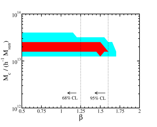
Figure 2.— Shaded regions show the 68% and 95% CL likelihood joint constraint on the slope $\beta$ of the density profile of $M>M_{c}$ halos and the mass $M_{c}$ separating the SIS and GNFW lenses. The results have been marginalized over all other parameters using WMAP priors. The vertical lines show the upper limits on $\beta$ after further marginalization over $M_{c}$.

Fig. 2 shows the joint constraints on $\beta$ and $M_{c}$ using the WMAP priors on $\Omega_{M}$ and $\sigma_{8}$ and the WMAP mean values for $n$, $\Omega_{M}h^{2}$ and $\Omega_{B}h^{2}$ that are determined very accurately. Although we have fixed $w=-1$ here, we have checked that the constraints are insensitive to $w$ by repeating the analysis for several values of $w$ and finding essentially identical results. The absence of $\theta\gtrsim 3^{\prime\prime}$ lenses in CLASS places an upper limit on the optical depth at these angular scales, which in turn limits how steep the inner cluster density profile can be: we find $\beta<1.25\,(1.60)$ at 68% (95%) CL (vertical lines) after marginalization over $M_{c}$. The constraints on $M_{c}$ are also strong due to the sudden break in the predicted optical depth at the angular separation corresponding to $M_{c}$ (see Fig. 1): we find $1.58<M_{c}/(10^{13}\,h^{-1}M_{\hbox{$\odot$}})<2.51$ at 68% CL and $1.25<M_{c}/(10^{13}\,h^{-1}M_{\hbox{$\odot$}})<3.98$ at 95% CL after marginalization over $\beta$.

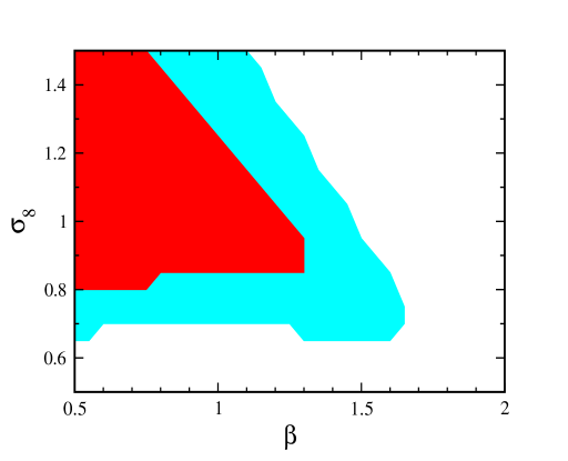
Figure 3.— 68% and 95% CL likelihood joint constraints on $\beta$ and $\sigma_{8}$ after marginalization over $M_{c}$ and $\Omega_{M}$.

Fig. 3 shows the joint constraints on $\beta$ and $\sigma_{8}$ using the same WMAP results as in Fig. 2 and after marginalization over $M_{c}$. It shows that steep density profiles ($\beta\sim 1.5$) are consistent with the absence of large-separation lenses only for a small range of low $\sigma_{8}$. High $\sigma_{8}$ ($\gtrsim 1$), on the other hand, is allowed by CLASS data provided the density profile is shallow. The lower limit of $\sigma_{8}>0.7$ at $95\%$ CL is insensitive to the value of $\beta$ because lowering $\sigma_{8}$ further would severely underpredict the cumulative optical depth at small image separations.

We have also attempted to obtain joint constraints on $\sigma_{8}$ and $w$ using the same WMAP parameters. After marginalizing over $\sigma_{8}$, our likelihood analysis gives $w<-0.75(-0.55)$ at 68% (95%) CL. The solid and double-dotted curves in Fig. 1, however, show that for two models with $w=-1$ and $-0.5$ but otherwise identical parameters, we would expect nearly identical number of lenses at $\theta<2^{\prime\prime}$ and at most a factor of two of difference at larger $\theta$. This insensitivity to $w$ is due to the fact that the matter power spectrum for different $w$ has identical shapes except on very large length scales (see, e.g., Ma et al. 1999), so once the models are normalized to the same $\sigma_{8}$ today, the only difference is in the growth rates at higher redshift and in $\Delta_{vir}$ for halo masses. (See Sarbu, Rusin & Ma 2001 for constraints on $w$ for COBE-normalized power spectrum.) The reason we were able to place any constraints on $w$ is because the theoretically computed optical depth for a fiducial (WMAP-favored) cosmology underpredicts the total optical depth, so that various models lie on the tail of the likelihood function. Since a more negative $w$ leads to a higher $\tau$, the total optical depth part of the likelihood function exponentially suppresses models with $w>-1$. We caution that constraints on $w$ (or any other parameters to which the test in question is only weakly sensitive) are robust only when the theoretically computed optical depth roughly agrees with the observation.

4. Discussion

We have used the statistics of the recently completed JVAS/CLASS radio survey to constrain the parameters in the two-population model of halos in the universe. Motivated by recent evidence from direct observations, $N$-body simulations, and semi-analytic arguments, we have assumed that all objects with mass less than $M_{c}$ have the SIS profile, while the more massive ones have the GNFW profile that scales as $r^{-\beta}$ in the inner region of the halos. The absence of $\theta\gtrsim 3^{\prime\prime}$ lenses in CLASS enables us to obtain tight constraints on $M_{c}$ and an upper limit $\beta<1.6$ at 95% CL. Furthermore, we obtain a constraint of $\sigma_{8}>0.7$ (95% CL) on the power spectrum normalization.

The constraints in our study have come from three effects: the total lensing optical depth measured by CLASS, the shape of the image separation distribution, and the lack of $\theta>3^{\prime\prime}$ lenses. It is therefore interesting to consider what happens when at least one large-separation event ($\gtrsim 5^{\prime\prime}$) is observed, and when such an event will be observed given our knowledge of the halo density profiles and cosmology. Keeton & Madau (2001) ask a similar question, and remark that one such large-separation event should be found in surveys such as the Two-Degree Field and Sloan Digital Sky Survey (SDSS), or else the cold dark matter model would have to be questioned. Fig. 1, however, shows that one could easily accommodate an extremely small probability of finding a large-separation event if, for example, we lived in a universe with $\sigma_{8}\sim 0.7$.

This issue may soon be resolved: there is evidence for a $\theta\approx 13^{\prime\prime}$ quadruple lens system in the SDSS (N. Inada et al., in preparation). Since this event is not yet a part of a controlled survey with significant statistics, it cannot be included in our analysis. To test how the constraint on $\beta$ would change with a positive detection of wide-separation lenses, we repeat our analysis by assuming a 14th lens in the statistical sample of JVAS/CLASS with $\theta=13^{\prime\prime}$ and a source at $z_{s}=2$. We find this hypothetical sample to favor $1.05<\beta<1.35$ at 68% CL, while tightening the constraint on $M_{c}$ with its central value unchanged. This result illustrates that stronger (lower as well as upper) limits on $\beta$ would be obtained if we had at least one large angular separation event in a controlled survey. This is simply because models with $\beta\lesssim 1$ predict $\ll 1$ lenses at large $\theta$ and would be strongly disfavored.

These factors motivate us to consider future surveys that may have enough statistics to detect large-separation lenses. The proposed LOw Frequency ARray (LOFAR; www.lofar.org) is expected to find millions of radio sources to fluxes below $1\mu Jy$ (Jackson 2002). Although the proposed angular resolution of $\sim 1^{\prime\prime}$ is inferior to that of CLASS, LOFAR would be a useful survey for detecting large-separation systems. Estimates from Jackson (2002) indicate that LOFAR would have 17,000 lenses in the brighter part of the survey with $30\sigma$ signal-to-noise ratio, providing a thousandfold increase in lensing statistics (if the identity of the lens events can be confirmed). Given the small number of lenses in current surveys, even if the LOFAR estimates are overly optimistic we can still expect that significantly larger statistical lens samples and other future wide-field telescopes such as SNAP (snap.lbl.gov) and LSST (www.dmtelescope.org/dark_home.html) will greatly improve our understanding of the populations of objects in the universe.

We thank Mike Kuhlen and Chuck Keeton for numerous useful suggestions and communicating their results prior to publication. We thank Josh Frieman for useful discussions. DH is supported by the DOE grant to CWRU. C-P Ma is supported by NASA grant NAG5-12173, a Cottrell Scholars Award from the Research Corporation, and an Alfred P. Sloan fellowship. A portion of this work was carried out at the Kavli Institute for Theoretical Physics.

References

- (1) Bullock, J. S. et al. 2001, ApJ, 550, 21
- (2) Browne, I.W.A. et al. 2003, MNRAS, 341, 13
- (3) Chae, K.-H. 2003, MNRAS, MNRAS, 346, 746
- (4) Chae, K.-H. et al. 2002, Phys. Rev. Lett., 89, 151301
- (5) Chen, D.-M. 2003, ApJ, 587, L55
- (6) Cheng, Y.-C. N. & Krauss, L. M. 2000, Int. J. Mod. Phys. A., 15, 697
- (7) Cohn, J.D., Kochanek, C.S., McLeod, B.A., & Keeton, C.R. 2001, ApJ, 554, 1216
- (8) Davis, A. N., Huterer, D. & Krauss, L. M. 2002, MNRAS, 344, 1029
- (9) Eisenstein, D. & Hu, W. 1997, ApJ, 511, 5
- (10) Jackson, N., “LOFAR and Gravitational Lenses” memorandum
- Jenkins et al. (2001) Jenkins, A. R. et al. 2001, MNRAS, 321, 372
- (12) Keeton, C. R., 1998, PhD. thesis, Harvard University
- (13) Keeton, C.R. & Madau, P. 2001, ApJ, 549, L25
- (14) King, L.J., Browne, I.W.A., Marlow, D.R., Patnaik, A.R., & Wilkinson, P.N. 1999, MNRAS, 307, 225
- (15) Kochanek, C. S. 1996, ApJ, 466, 638
- (16) Kochanek, C. S. & Blandford, R. 1987, ApJ, 321, 676
- (17) Kuhlen, M., Keeton, C.R. & Madau, P. 2003, ApJ, in press
- (18) Li, L.-X. & Ostriker, J. P. 2002, ApJ, 566, 652
- (19) Li, L.-X. & Ostriker, J. P. 2003, ApJ, 595, 603
- (20) Ma, C.-P. 2003, ApJ, 584, L1
- (21) Ma, C.-P., Caldwell, R.R., Bode, P. & Wang, L. 1999, ApJ, 521, L1
- (22) Marlow, D.R. et al. 2000, AJ, 119, 2629
- (23) Moore, B., Quinn, T., Governato, F., Stadel, J. & Lake, G. 1999, MNRAS, 310, 1147
- (24) Myers, S.T., et al. 2003, MNRAS, 341, 1
- (25) Navarro, J.F., Frenk, C.S. & White, S.D.M. 1997, ApJ, 490, 493
- (26) Oguri, M., Taruya, A. & Suto, Y. 2001 ApJ, 559, 572
- (27) Oguri, M., Taruya, A., Suto, Y. & Turner, E.L. 2002, ApJ, 568, 488
- (28) Phillips, P.M., et al. 2001, MNRAS, 328,1001
- (29) Porciani, C. & Madau, P. 2000, ApJ, 532, 679
- (30) Rusin, D., Kochanek, C.S. & Keeton, C.R. 2003, ApJ, 595, 29
- (31) Rusin, D., & Ma, C.-P. 2001, ApJ, 549L, 33
- (32) Rusin, D. & Tegmark, M. 2001, ApJ, 553, 709
- (33) Sand, D., Treu, T., & Ellis, R. 2002, ApJ, 574, L129
- (34) Sarbu, N., Rusin, D., & Ma, C.-P. 2001, ApJ, 561, L147
- (35) Spergel, D.N. et al. 2003, ApJ, 148S, 175
- (36) Takahashi, R. & Chiba, T. 2001, ApJ, 563, 489
- (37) Treu, T. & Koopmans, L.V.E. 2002, ApJ, 575, 87
- (38) Turner, E. L. 1990, ApJ, 365, L43
- (39) Turner, E. L., Ostriker, J.P., & Gott, J.R. 1984, ApJ, 284, 1
- (40) Wallington, S. & Narayan, R. 1993, ApJ, 403, 517
- (41) Weinberg, N. & Kamionkowski, M. 2003, MNRAS, 341, 251
- (42) Winn, J., Rusin, J. & Kochanek C.S. 2003, ApJ, 587, 80
- (43) Zhao, H. S. 1996, MNRAS, 278, 488