Contributions of point extragalactic sources
to the Cosmic Microwave Background bispectrum

Abstract

All the analyses of Cosmic Microwave Background (CMB) temperature maps up–to–date show that CMB anisotropies follow a Gaussian distribution. On the other hand, astrophysical foregrounds which hamper the detection of the CMB angular power spectrum, are not Gaussian distributed on the sky. Therefore, they should give a sizeable contribution to the CMB bispectrum. In fact, the first year data of the Wilkinson Microwave Anisotropy Probe (WMAP) mission have allowed the first detection of the extragalactic source contribution to the CMB bispectrum at 41 GHz and, at the same time, much tighter limits than before to non–Gaussian primordial fluctuations. In view of the above and for achieving higher precision in current and future CMB measurements of non–Gaussianity, in this paper we discuss a comprehensive assessment of the bispectrum due to either uncorrelated or clustered extragalactic point sources in the whole frequency interval around the CMB intensity peak.

Our calculations, based on current cosmological evolution models for sources, show that the reduced angular bispectrum due to point sources, $b_{ps}$, should be detectable in all WMAP and Planck frequency channels. We also find agreement with the results on $b_{ps}$ at 41 GHz coming from the analysis of the first year WMAP data . Moreover, by comparing $b_{ps}$ with the primordial reduced CMB bispectrum, we find that only the peak value of the primordial bispectrum (which appears at $l\simeq 200$) results greater than $b_{ps}$ in a frequency window around the intensity peak of the CMB. The amplitude of this window basically depends on the capability of the source detection algorithms (i.e., on the achievable flux detection limit, $S_{lim}$, for sources). Finally, our current results show that, at low frequencies (i.e., $\nu\leq 100$ GHz), the angular bispectrum of a clustered distribution of sources appears not substantially different from that of Poisson distributed ones, by using realistic angular correlation functions suitable to be applied to the relevant source populations. On the other hand, we also find that at higher frequencies (i.e., $\nu\geq 300$ GHz), the clustering term can greatly enhance the normalization of $b_{ps}$.

1 INTRODUCTION

The analysis of the first year Wilkinson Microwave Anisotropy probe (WMAP) data clearly show that temperature fluctuations of the Cosmic Microwave Background (CMB) follow a Gaussian distribution (Komatsu et al., 2003; Spergel et al., 2003) in agreement with the standard inflation paradigm. Therefore, the third moment of this distribution and its angular bispectrum, $C_{{l_{1}}{l_{2}}{l_{3}}}$, the harmonic transform of the three–point correlation function, should be zero and the angular power spectrum, $C_{\ell}$, specify all the statistical properties of CMB anisotropy. Anyway, significant non-Gaussianity can be introduced, for instance, by second order relativistic effects or by features in the scalar field potential, which can produce an angular bispectrum potentially detectable in all–sky maps as those provided by the WMAP and Planck satellite missions (Bennett et al., 2003a; Mandolesi et al., 1998; Puget et al., 1998).

In the standard inflationary scenario, the quantum fluctuations of the scalar field are the origin of the matter and radiation fluctuations in the Universe. In slow-roll inflation, weak non-Gaussian fluctuations are generated by non-linearity in inflation (Salopek and Bond, 1990) or by features appearing in the inflation potential (Gangui et al., 1994) which can produce small deviations from gaussianity in the CMB temperature fluctuations. Second order relativistic effects can give also rise to a detectable non-Gaussian contribution (Pyne and Carroll, 1996). All these effects can be summarized by the following expression for the curvature perturbations,

$$\Phi(x)=\Phi_{L}(x)+f_{nl}\,(\Phi_{L}^{2}(x)-\langle\Phi_{L}^{2}(x)\rangle).$$ (1)

where $\Phi_{L}(x)$ is the Gaussian part of the perturbations, $f_{nl}$ is the non-linear coupling parameter, given by a certain combination of the slope and the curvature of the inflaton potential, and $\langle\rangle$ means the statistical ensemble average (Falk, Rangarajan, and Srednicki 1993; Gangui et al. 1994; Wang and Kamionkowski 2000). In general, high values of $f_{nl}$ can be obtained just with a small tilt of the spectrum and these values could give rise to a bispectrum signal potentially detectable in current as well as future all sky CMB maps. Moreover, the value of $f_{nl}$ could be also increased by deviations from standard inflationary models (see, e.g., Kofman et al. 1991).

The great astrophysical interest in the detection of primordial non–Gaussianity has stimulated the development of many different methods suitable in analyzing CMB anisotropy: Minkowski functionals on the sphere (Schmalzing and Gorski 1998), statistics of excursion sets (Barreiro et al. 2001), wavelets (Pando et al. 1998; Barreiro et al. 2000; Cayón et al. 2001), the bispectrum (Luo 1994; Komatsu and Spergel, 2001; Komatsu et al. 2002; Santos et al. 2002). The main result of all these analyses is that no positive detection of non-Gaussianity in CMB maps has been confirmed up to now: COBE DMR (Bromley and Tegmark, 1999; Cayón et al., 2003; Komatsu et al., 2002) Maxima-1 (Wu et al. 2001; Santos et al. 2002) and Boomerang (Polenta et al. 2001) data appear all compatible with the Gaussian hypothesis. On the other hand, Ferreira et al. (1998) have measured 9 equilateral modes $(\ell_{1}=\ell_{2}=\ell_{3})$ of the normalized bispectrum, $B_{{l_{1}}{l_{2}}{l_{3}}}/C_{\ell}^{1/2}$, on the COBE DMR map, claiming detection at $\ell_{1}=\ell_{2}=\ell_{3}=16$ whereas Bromley and Tegmark (1999) find that few individual pixels – which could be contaminated by both foreground emission and instrumental noise – are responsible of most of the claimed primordial signal.

A great challenge to precise measurements of non–Gaussianity in the CMB is set by astrophysical foregrounds which constitute an unavoidable limitation : see, e.g., “Microwave Foregrounds”, 1999, A. de Oliveira Costa and M. Tegmark eds., ASP Conf. Ser. Vol.181, for a thorough discussion on the subject. At present, even applying the most efficient methods for component separation, the residual astrophysical signal – which is not, in general, Gaussian distributed – can contaminate a non negligible number of pixels giving rise to a detectable contribution to non–Gaussianity. Other studies have discussed the effect of Galactic foregrounds on non–Gaussianity (see, e.g., Komatsu et al., 2002). In this paper, we focus on extragalactic point sources whose contribution to CMB anisotropies has been analyzed in detail (Toffolatti et al. 1998; Sokasian et al., 2001; Park, Park & Ratra 2002) whereas their contribution to the CMB bispectrum has been poorly studied up to now. A first estimate of the reduced bispectrum, $b_{ps}$, due to Poisson distributed point sources at two frequencies only (90 and 217 GHz) has been recently presented by Komatsu & Spergel (2001), hereafter KS01. This paper has shown that undetected point sources, i.e. sources at fluxes below the detection threshold of the experiment, give rise to a non zero $b_{ps}$ value which could hamper the detection of the primordial signal. Very recently, by the analysis of the first year WMAP observations, Komatsu et al. (2003) have claimed the first detection of the bispectrum due to extragalactic sources. In view of the above, it is clearly of great interest to perform a thorough analysis of the contribution of point sources to the CMB bispectrum. Therefore, we extend the calculation of KS01 to the whole frequency range of the WMAP and Planck missions, using model number counts able to reproduce the data available so far. Moreover, we take also into account the effect of correlated positions of point sources in the sky for studying how much source clustering can enhance the value of the reduced angular bispectrum, $b_{ps}$.

The outline of the paper is as follows. In Section 2 we briefly summarize the formalism used to estimate the reduced bispectrum and show detailed calculations of its value due to Poisson distributed point extragalactic sources. In Section 3, we model the clustering properties of sources at microwave frequencies by 2D simulations and we present the first estimates to date of the CMB bispectrum produced by clustered sources. Finally, in Section 4, we discuss our main results and present the conclusions. We assume a standard Cold Dark Matter (CDM) cosmology ($\Omega_{M}$=1.0, $H_{0}=50$ km/s/Mpc) but we discuss our findings also in the case of a flat $\Lambda$CDM model with $\Omega_{M}=0.3$ and $\Omega_{\Lambda}=0.7$. Anyway, as discussed below, the conclusions are largely independent of the adopted cosmological model.

2 THE BISPECTRUM DUE TO UNCLUSTERED POINT SOURCES

2.1 General formalism

CMB temperature fluctuations ${\Delta T(\mathbf{n})}/{T}$ are usually expanded into spherical harmonics

$$a_{lm}=\int_{\Omega}d^{2}{\mathbf{n}}\ \frac{\Delta T(\mathbf{n})}{T}Y_{lm}^{\ast}(\mathbf{n})\,$$ (2)

where $\Omega$ denotes the full sky (in the case of an incomplete sky coverage, the integral is done over the observed sky area, $\Omega_{obs}$; see, e.g., Komatsu et al., 2002). The angular third moment of CMB temperature fluctuations is defined as

$$B_{l_{1}l_{2}l_{3}}^{m_{1}m_{2}m_{3}}\equiv{\langle a_{l_{1}m_{1}}a_{l_{2}m_{2}}a_{l_{3}m_{3}}\rangle}$$ (3)

and the averaging is over the ensemble of realizations. If the fluctuations are gaussian distributed, the third moment and all the higher order moments are zero.

Due to the rotational invariance of the universe

$$B_{l_{1}l_{2}l_{3}}^{m_{1}m_{2}m_{3}}=\left(\begin{array}[]{c c c}l_{1}&l_{2}&l_{3}\\ m_{1}&m_{2}&m_{3}\end{array}\right)C_{l_{1}l_{2}l_{3}}$$ (4)

where $C_{l_{1}l_{2}l_{3}}$ is the angular bispectrum and the matrix is the Wigner-3j symbol. Since we only have access to one sky we need an estimator of the angular bispectrum: the best unbiased estimator (Gangui and Martin 2000) is the angle–averaged bispectrum

$$B_{l_{1}l_{2}l_{3}}\equiv\sum_{m_{1}m_{2}m_{3}}\left(\begin{array}[]{c c c}l_{1}&l_{2}&l_{3}\\ m_{1}&m_{2}&m_{3}\end{array}\right)B_{l_{1}l_{2}l_{3}}^{m_{1}m_{2}m_{3}}$$ (5)

Another related quantity is the reduced bispectrum $b_{l_{1}l_{2}l_{3}}$, which can be expressed easily in terms of the angular bispectrum

$$C_{l_{1}l_{2}l_{3}}=\sqrt{\frac{(2l_{1}+1)(2l_{2}+1)(2l_{3}+1)}{4\pi}}\times\left(\begin{array}[]{c c c}l_{1}&l_{2}&l_{3}\\ m_{1}&m_{2}&m_{3}\end{array}\right)b_{l_{1}l_{2}l_{3}}$$ (6)

and which contains all the physical information in $B_{l_{1}l_{2}l_{3}}^{m_{1}m_{2}m_{3}}$. The reduced bispectrum can also be related to the third moment

$${\langle a_{l_{1}m_{1}}a_{l_{2}m_{2}}a_{l_{3}m_{3}}\rangle}={\cal G}_{l_{1}l_{2}l_{3}}^{m_{1}m_{2}m_{3}}\,b_{l_{1}l_{2}l_{3}}$$ (7)

where ${\cal G}_{l_{1}l_{2}l_{3}}^{m_{1}m_{2}m_{3}}$ is the Gaunt integral

$${\cal G}_{l_{1}l_{2}l_{3}}^{m_{1}m_{2}m_{3}}=\int d^{2}({\mathbf{n}})Y_{l_{1}m_{1}}({\mathbf{n}})\,Y_{l_{2}m_{2}}({\mathbf{n}})\,Y_{l_{3}m_{3}}({\mathbf{n}})$$ (8)

The reduced angular bispectrum is a very convenient quantity, since it can be easily calculated in the flat two-dimensional approximation (Santos et al. 2001).

Having summarized the general formalism, we remind here the calculation of the reduced bispectrum expected in the case of unclustered point sources, i.e extragalactic point–like sources which follow a Poisson distribution in the sky. Toffolatti et al. (1998) found that this assumption is fairly good at microwave frequencies, if sources are not subtracted down to very faint flux limits, thus greatly decreasing Poisson fluctuations whereas leaving almost unaffected the clustering term. Under this assumption, the sky distribution of extragalactic sources produces a white noise spectrum and, from Eq.(7), we define

$$b_{ps}\equiv b_{l_{1}l_{2}l_{3}}^{sources}={\langle(T-\langle T\rangle)^{3}\rangle/T^{3}}$$ (9)

i.e., equal to the skewness of the sky temperature distribution. Therefore, $b_{ps}$=constant at all scales $\ell$.

The reduced bispectrum, $b_{ps}$, can be then calculated as follows

$$b_{l_{1}l_{2}l_{3}}=g^{3}(x)\int_{0}^{S_{lim}}dS\,S^{3}\,\frac{dn}{dS}$$ (10)

where $\displaystyle\frac{dn}{dS}$ is the differential source count per unit solid angle, $S$ the flux and $g$ the conversion factor from fluxes to temperatures

$$g(x)\equiv 2\frac{(hc)^{2}}{(k_{B}T)^{3}}\frac{(sinh{x}/{2}))^{2}}{x^{4}}$$ (11)

where $x\equiv h\nu/k_{B}T$. The integral in Eq.(10) has to be computed up to the flux detection limit foreseen for the experiment, $S_{lim}$, since only undetected sources are contributing to the estimated $b_{ps}$.

2.2 Number counts of extragalactic sources

To perform the integral in Eq. (10) we have used the differential counts corresponding to the cosmological evolution models for radio and far–IR selected sources discussed in Toffolatti et al. (1998) (hereafter TO98). This choice represent a clearly better approximation than simple power law counts, as assumed by KS01 with the purpose of obtaining a first estimate of $b_{ps}$. However, since they used the model counts of TO98 for the extrapolation of source counts at 94 GHz, with the flux detection threshold of $S_{lim}\simeq 2$ Jy (the estimated $5\sigma$ detection limit of WMAP W-band), it is not surprising that their estimates result in good agreement with our current ones.

As for data on radio counts, preliminary measurements at 15.2 GHz by Taylor et al. (2001) suggested that the extrapolation of the model counts of TO98 – which successfully account for the observed source counts down to $S\sim 0.1$ mJy in flux and up to 8.44 GHz – overestimates their data by a factor of $\sim 1.5\div 2$ at the survey limit ($\simeq 20$ mJy), implying that the simple assumptions on source spectra and/or on cosmological evolution could not have been the most correct ones. On the other hand, the recently published WMAP analysis of the foreground emission (Bennett et al., 2003b) has provided a full sky catalogue of 208 bright extragalactic sources with fluxes $S\geq 0.9-1.0$ Jy, of which only five objects could be spurious identifications. The whole sample give an average flat ($\alpha=0.0\pm 0.2$) energy spectrum in full agreement with the assumptions of TO98 and number counts of bright sources at 41 GHz which appear to fall below the prediction of TO98 at 30 GHz by a factor of $\sim 0.66$ (but only in the faintest flux bins). Direct calculations of the 33 GHz counts by the source catalogue in Table 5 of Bennett et al. (2003b) give 155 sources at $S_{lim}\simeq 1.25$ Jy on a sky area of 10.38 sr ($|b^{II}|>10^{\circ}$) where the sample appears to be statistically complete. By this sample we could estimate again the WMAP differential counts finding an average offset of $\sim 0.75$ with the TO98 model predictions (see Toffolatti et al. (2003) for more details).

Moreover, two other recently published independent samples of extragalactic sources at 31 and 34 GHz – from CBI (Mason et al., 2003) and VSA (Taylor et al., 2003) experiments, respectively – show that the TO98 model correctly predicts number counts down to, at least, $S\simeq 10$ mJy. Another independent check of the assumptions of the TO98 model is coming from the few detections of extragalactic point sources in the Boomerang maps. These sources show flat or decreasing spectra up to 240 GHz (Coble et al., 2003) which is again in agreement with the population mixture of TO98. Therefore, given that almost all up–to–date observations are confirming the predictions on source counts of the TO98 model up to 30-34 GHz, we can be very confident in applying this model for our current predictions, at least up to frequencies $\leq 100\div 150$ GHz, where “flat”–spectrum sources dominate the bright counts.

On the other hand, a lot of new data on far–IR/sub–mm source counts have piled up since 1998, in particular by means of the SCUBA and MAMBO surveys. These current data are better explained by new physical evolution models of far–IR selected sources, as the ones presented by Guiderdoni et al. (1998) and by Granato et al. (2001). Therefore, we also compare our first estimate of $b_{ps}$ at 545 GHz with the ones obtained by directly integrating the differential counts of these two latter predictions. Anyway, since the reduced bispectrum due to undetected sources is produced by all sources below a given detection limit, the integral in eq. (10) results not much affected by the adopted evolution model (see below).

In Table 1 we present our current estimates of the reduced bispectrum, $b_{ps}$, due to Poisson distributed extragalactic sources at various frequencies in the range 15–850 GHz and applying different flux limits, $S_{lim}$, for source detection. The frequencies and flux detection limits has been chosen to directly compare with those of the MAP and Planck satellite missions. All our estimates have been calculated by taking into account both the radio and far–IR source populations at each frequency channel. Anyway, at frequencies below $\sim 150$ GHz the contribution of far–IR selected sources is negligible whereas at $\nu\geq$500 GHz the same applies to radio selected ones. The values of $b_{ps}$ are, obviously, at a minimum close to the CMB intensity peak where bright sources reach a minimum number.

It is worthy to remind that the first estimate of KS01 gave the value $b_{ps}\sim 2\times 10^{-25}$ at 94 GHz, with $S_{lim}\sim 2$ Jy whereas our current estimate is $\sim 3.7\times 10^{-25}$; at 217 GHz and with $S_{lim}\sim 0.2$ Jy their value was $\sim 5\times 10^{-28}$ whereas we obtain $\sim 3.8\times 10^{-28}$. The general agreement and, at the same time, the little mismatch with our estimates are not surprising since KS01 used the TO98 model for estimating $b_{ps}$ but they extrapolated TO98 number counts with a constant slope down to faint fluxes.

Table 1: Sample values of $b_{ps}$ in the 15–850 GHz frequency interval and for different flux detection limits, $S_{lim}$. All the Planck channels are indicated.

$\nu$(GHz)	$S_{lim}=2.$ Jy	$=1.$ Jy	$=0.1$ Jy	$=0.01$ Jy
15	$1.5\times 10^{-20}$	$5.0\times 10^{-21}$	$0.9\times 10^{-22}$	$1.0\times 10^{-24}$
23	$7.8\times 10^{-22}$	$2.6\times 10^{-22}$	$4.6\times 10^{-24}$	$5.0\times 10^{-26}$
30	$1.9\times 10^{-22}$	$6.4\times 10^{-23}$	$1.2\times 10^{-24}$	$1.4\times 10^{-26}$
44	$2.2\times 10^{-23}$	$7.2\times 10^{-24}$	$1.3\times 10^{-25}$	$1.4\times 10^{-27}$
61	$3.6\times 10^{-24}$	$1.1\times 10^{-24}$	$1.7\times 10^{-26}$	$1.9\times 10^{-28}$
70	$1.6\times 10^{-24}$	$5.3\times 10^{-25}$	$8.8\times 10^{-27}$	$1.0\times 10^{-28}$
94	$3.7\times 10^{-25}$	$1.2\times 10^{-25}$	$1.9\times 10^{-27}$	$2.2\times 10^{-29}$
100	$2.8\times 10^{-25}$	$9.0\times 10^{-26}$	$1.5\times 10^{-27}$	$1.8\times 10^{-29}$
143	$4.5\times 10^{-26}$	$1.5\times 10^{-26}$	$2.8\times 10^{-28}$	$4.5\times 10^{-30}$
217	$1.6\times 10^{-26}$	$5.7\times 10^{-27}$	$1.6\times 10^{-28}$	$8.0\times 10^{-30}$
353	$1.6\times 10^{-25}$	$7.0\times 10^{-26}$	$5.5\times 10^{-27}$	$4.0\times 10^{-28}$
545	$2.0\times 10^{-22}$	$1.0\times 10^{-22}$	$7.8\times 10^{-24}$	$3.0\times 10^{-25}$
857	$1.0\times 10^{-16}$	$4.8\times 10^{-17}$	$2.6\times 10^{-18}$	$5.6\times 10^{-20}$

It is also interesting to compare $b_{ps}$ estimates with the reduced CMB bispectrum obtained in non-Gaussian models with fluctuations of the inflation potential given by eq. (1). This quantity has also been carefully calculated by KS01. They have shown that the equilateral bispectrum $b_{lll}$ – i.e., the reduced angular bispectrum $b_{l_{1}l_{2}l_{3}}$ when $l_{1}=l_{2}=l_{3}$ – multiplied by $l^{4}$ exhibits a peak at multipole $\ell\simeq 200$. The height of this peak is proportional to the factor $f_{nl}$, the coupling parameter.

In Figure 1 we also compare our estimates of $b_{ps}$ with the primordial CMB equilateral bispectrum, $b_{lll}$, at its peak value ($\ell\simeq 200$) by adopting $f_{nl}=100,10,1$. As also indicated in Table 1, we explore the whole frequency interval around the intensity peak of the CMB. Looking at Figure 1, the peak value of the primordial $b_{lll}$ appears greater than $b_{ps}$ in a frequency window around the CMB intesity peak: obviously, the window sets larger by increasing the value of $f_{nl}$ and by reducing the source detection limit, $S_{lim}$. If $f_{nl}=100$ and with $S_{lim}\simeq 0.1$ Jy, the window spans from $\sim 30$ to $\sim 500$ GHz. On the other hand, if $f_{nl}=10$ and $S_{lim}\simeq 2$ Jy, the window shrinks to $100\leq\nu\leq 350$ GHz. The line corresponding to $f_{nl}=1$ is plotted only as a reference, since the ideal experiment requires $f_{nl}>3$, in order to obtain $S/N>1$ (Komatsu and Spergel, 2001).

As an example, in Figure 2 we show our estimates of $b_{ps}$ at three frequencies, 30, 44 and 70 GHz, and for $S_{lim}$=1,0.1 Jy comparing them with the primordial equilateral bispectrum, $b_{lll}$, calculated by assuming $f_{nl}=10$. It is apparent that at this three frequencies, and, thus, for all frequencies below $\nu\simeq 70\div 80$ GHz, $b_{ps}$ has always a higher value than the primordial CMB bispectrum if $S_{lim}\geq 1$ Jy. On the other hand, if we are able to detect and remove sources brighter than $S_{lim}\simeq 0.1$ Jy, which could be attaineable by Planck (Vielva et al., 2003), the peak value of the primordial CMB bispectrum should be detectable at frequencies $\nu\geq 40\div 50$ GHz, for this choice of $f_{nl}$. We checked that fixing $f_{nl}=100$, the limits for the detectability of the primordial bispectrum move down in frequency to $\sim 50$ and $\sim 20$ GHz, if $S_{lim}=1,0.1$ Jy, respectively. We have limited our comparisons to these values of $f_{nl}$ since WMAP data (Komatsu et al., 2003) already imply that $f_{nl}\leq 134$, at the 95% confidence level.

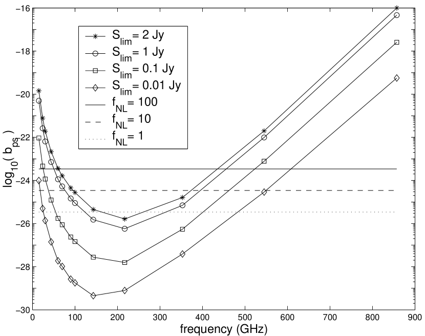
Figure 1: Reduced equilateral bispectrum, $b_{ps}$, due to Poisson distributed point sources in the 15–900 GHz frequency interval and for several flux detection limits, $S_{lim}$, for sources. The peak value of the primordial CMB bispectrum (at $\ell\sim 200$) generated by a quadratic potential is also plotted for different values of the coupling parameter, $f_{nl}$.

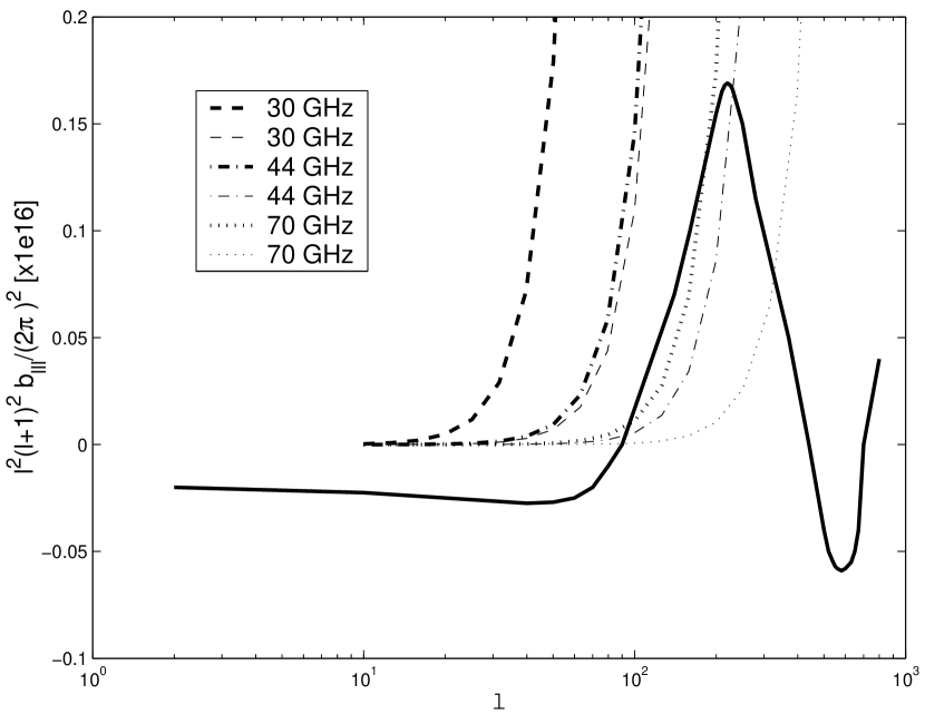
Figure 2: Comparison of the reduced CMB bispectrum, in terms of $\sim\ell^{4}b_{lll}$, for $f_{nl}=10$, thick continuous line, with the estimates of $b_{ps}$ given by Poisson distributed sources at 30, 44 and 70 GHz and with $S_{lim}=1$ (thick dashed, point-dashed and dotted lines, respectively). We also plot the result with $S_{lim}=0.1$ Jy, thin lines.

As shown by KS01, the contribution of point sources and the one coming from the Sunyaev-Zeldovich effect can be separated from the primordial CMB angular bispectrum via chi-square minimization, by taking into account the different shape of the three contributions and thanks to the sensitivity of satellite observations. According to Table 3 in their paper, the signal-to-noise ratios for $b_{ps}$ are $2.2\times 10^{25}b_{ps}$ for WMAP and $52\times 10^{27}b_{ps}$ for Planck, respectively. The source contribution to the CMB bispectrum should therefore be detectable by WMAP if $b_{ps}\geq 2\times 10^{-25}$ (4$\sigma$ limit) and, more easily, by Planck since it should be sufficient that $b_{ps}\geq 10^{-28}$ (4$\sigma$), in this latter case. A comparison of the above detection limit for Planck with our current estimates of Table 1 shows that $b_{ps}$ should be detectable in all Planck channels even lowering the source detection limit down to $S_{lim}\sim 0.1$ Jy, which currently appears as an achievable limit, at least for all frequencies below $\sim 200$ GHz (Vielva et al., 2003). If we take the WMAP limit, we find that $b_{ps}$ could be detected also at all WMAP frequencies (only at $1\div 2\sigma$ level in the 94 GHz channel) if only sources not fainter than $S_{lim}\sim 1.0$ Jy are detected and removed. This appears as a realistic possibility given that only very few sources in Table 5 of Bennett et al. (2003b) show fluxes $S<0.9\div 1.0$ Jy.

Very recently, Komatsu et al. (2003) published the first detection of $b_{ps}$ at microwave frequencies: they report the value of $(9.5\pm 4.4)\times 10^{-5}$ $\mu K^{3}$sr², by adopting $S_{lim}\simeq 0.75$ Jy for source detection in the 41 GHz WMAP channel. Our current findings are in good agreement with the claim of Komatsu et al. (2003): in fact, by directly integrating the differential source counts of TO98 up to $S_{lim}=0.75$ Jy at 41 GHz, we find $b_{ps}\simeq 13\div 14\times 10^{-5}$ $\mu K^{3}$sr², where the scatter is due to the different cosmology ($\Omega_{M}=1.0$ or $\Omega_{M}=0.3$). These results are compatible with the detection of Komatsu et al. (2003) at $1\sigma$ level whereas we have to apply a correction factor of $\simeq{0.7}$ for obtaining the best fit value of Komatsu et al. (2003). If we use the more realistic value of $S_{lim}\simeq 1.0$ Jy (see Section 2) for source detection we find $b_{ps}\simeq 20\div 22\times 10^{-5}$ $\mu K^{3}$sr² in the Q band. On the other hand, by integrating the TO98 model counts at 61 GHz (WMAP V band) up to $S_{lim}=0.75$ Jy we obtain $b_{ps}\simeq 1.3\div 1.4\times 10^{-5}$ $\mu K^{3}$sr², showing a reduced scatter of $\simeq 0.80$ with the Komatsu et al. (2003) best fit value (see their Table 1). Moreover, Hinshaw et al. (2003) have found an excess angular power spectrum $C_{\ell}=(15.5\pm 1.7)\times 10^{-3}$ $\mu K^{2}$sr at small scales, which they explain as produced by undetected point sources, in agreement with the findings of Komatsu et al. (2003) . Again, by adopting $S_{lim}=$0.75 and 1.0 Jy for source detection, our current estimates at 41 GHz give $C_{\ell}\simeq$ 20 and 24.0 $\mu K^{2}$sr, respectively, showing a similar offset as for the point source bispectrum. Again, in the V band we obtain $C_{\ell}\simeq 4.5\div 5.0\times 10^{-3}$ $\mu K^{2}$sr with $S_{lim}=0.75$ in much better agreement with the Komatsu et al. (2003) estimate of $(4.5\pm 4)\times 10^{-3}$ $\mu K^{2}$sr. As a result, and in agreement with Komatsu et al. (2003) we actually find an offset between their current results and our estimates of $b_{ps}$. Anyway, Komatsu et al. (2003) results and our current estimates – obtained by directly integrating the TO98 differential counts – are consistent at the $1\sigma$ level and, moreover, in the V band the offset ($\sim 0.8\div 0.9$) is smaller than in the Q band.

Finally, it is important to remind that all these estimates have been computed by adopting a Poisson distribution of sources in the sky and a standard CDM cosmology with $\Omega_{M}=1.0$. Anyway, our current result are not very much affected by the cosmology: in fact, if we use a flat $\Lambda$CDM model ($\Omega_{\Lambda}=0.7$), our estimates only increases of a factor $\simeq 1.1\div 1.25$ in the 15–150 GHz frequency interval and by a slightly greater factor ($\simeq 1.5\div 2.3$) at higher frequencies, while keeping the same parameters as in TO98 for the cosmological evolution of sources.

3 THE BISPECTRUM DUE TO CLUSTERED POINT SOURCES

TO98 found that the clustering contribution to CMB fluctuations due extragalactic sources is generally small in comparison with the Poisson one. On the other hand, if clustering of sources at high redshift is very strong it can give rise to a power spectrum stronger than the Poisson one (Perrotta et al., 2003; Scott and White, 1999). We remind, however, that current models (Toffolatti et al., 1998; Guiderdoni et al., 1998) suggest a broad redshift distribution of extragalactic sources contributing to the CMB angular power spectrum, implying a strong dilution of the clustering signal (Toffolatti et al., 1999). Anyway, in view of extracting the most precise information from current and future CMB data, i.e. pursuing precision cosmology, it is also important to assess to which extent the clustering signal can reduce the detectability of the primordial CMB bispectrum.

In a companion paper (Toffolatti et al., 2003) we have addressed the problem of estimating the CMB angular power spectrum given by undetected clustered point sources by adopting a simple phenomenological approach. In that paper we exploit the very few data available so far on the angular correlation function of radio and far-IR selected sources to estimate the $C_{\ell}$ of extragalactic sources at microwave frequencies. We use here the same approach and the same simulated maps to estimate the clustering contribution to $b_{ps}$ as previously done for the Poisson case. We focused on WMAP and Planck LFI channels, at which extragalactic radio sources, displaying a ”flat” energy spectrum (Bennett et al., 2003b), dominate the bright counts. We also give a first estimate of $b_{ps}$ at 545 GHz (a Planck HFI channel) and we defer to a future paper (González-Nuevo et al., 2003) for a most comprehensive multifrequency analysis.

We briefly remind here the adopted procedure. We have carried out 100 simulations in 2D–flat patches of the sky of $12^{\circ}.8\times 12^{\circ}.8$ and $25^{\circ}.6\times 25^{\circ}.6$ deg² and with a pixel size of $\sim$1.5 arcmin for Planck and of $\sim$6 arcmin for WMAP, since maps are created in the HEALPix format with $nside=512$ (Gorski et al., 1998) in this latter case. A different pixel size can highly increase/decrease the pixel-by-pixel variance in presence of a strong clustering signal, and the effect has to be taken into account. In this case, at WMAP and LFI frequencies, the effect proves negligible in agreement with the previous findings of Toffolatti et al. (1998).

As discussed in more detail elsewhere (Toffolatti et al., 2003), we first distribute point sources at random in the sky with their total number fixed by the integral counts, $N(>S)$, of the TO98 model at each given frequency. We then calculate the Fourier transform of the density contrast map, i.e. the map defined by $\delta(\vec{x})\equiv{N(\vec{x})-<N>\over<N>}$, where $\langle N\rangle$ is the average number of sources per pixel, obtaining a “white noise” power spectrum, $P(\mathbf{k})_{Poiss}=<|\delta_{k}|^{2}>$, thus normalized to the total number of sources foreseen by the model. The next step has been to modify this normalized spectrum by the Fourier tranform of the angular correlation function, $w(\theta)$, corresponding to the appropriate source population. We adopt here the $w(\theta)$ measured at 4.85 GHz by Loan, Wall and Lahav (1997), since the source population of bright sources ($S>50$ mJy) which has been sampled at this frequency is representative also of bright sources seen at higher frequencies: the underlying parent population appears to be the same one (Bennett et al., 2003b) in agreement with the assumption of the TO98 model. Other estimates of $w(\theta)$ for radio sources come from samples at lower frequencies (e.g., 1.4 GHz) and down to lower fluxes where the dominant source populations are different from the ones relevant for WMAP and Planck observations.

With this choice of $w(\theta)$ the modified density contrast of each pixel in the Fourier space is

$$\delta_{k}(corr)=\delta_{k}\sqrt{P(\mathbf{k})_{Poiss}+P(\mathbf{k})_{cl}\over P(\mathbf{k})_{Poiss}}$$ (12)

where $P(\mathbf{k})_{cl}$ is the Fourier transform of the chosen $w(\theta)$. In this way the source density is modified by the adopted correlation function whereas the normalization to the total effective number of sources predicted by the model remains fixed by $\langle N\rangle$. By the 2D Fourier antitransform we get again the map in the real space (the sky patch). As discussed in detail by Toffolatti et al. (2003), the procedure is “safe” since the total number of sources and the number counts remain unchanged whereas the recovered $w(\theta)$ matches very well the input one. We want to stress here that this is a phenomenological approach, since we are currently interested in reproducing the observational angular correlation functions of the relevant source populations, if they are available.

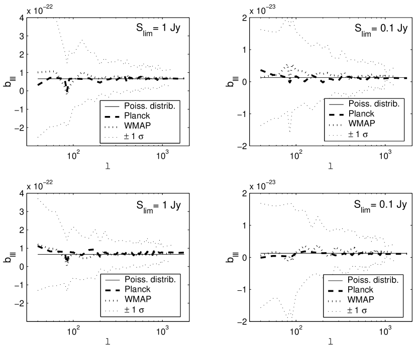
Figure 3: Reduced equilateral bispectrum, $b_{ps}$, at 30 GHz for two different source detection limits. In each panel, the straight horizontal line represents the $b_{ps}$ value of Table 1., obtained by directly integrating Eq.(10) and, thus, using a Poisson distribution of sources in the sky. For comparison, we also plot the $b_{ps}$ values obtained by averaging over 100 simulations of clustered point sources, upper panels, and of Poisson distributed sources, lower panels, at the Planck and WMAP resolutions (see text). In the case of WMAP we actually performed the simulations at 33 GHz. The $\pm 1\sigma$ limits refer to the set of simulations at the WMAP resolution limit.

Finally, from the simulated maps, in terms of $\Delta T/T$, we then obtain the Fourier transform

$$a({\mathbf{k}})=\int\frac{\Delta T(\mathbf{r})}{T}e^{-i{\mathbf{kr}}}\,d^{2}{\mathbf{r}}$$ (13)

and the calculation of the bispectrum in the 2D flat-sky approximation is given by

$$<a({\mathbf{k_{1}}})a({\mathbf{k_{2}}})a({\mathbf{k_{3}}})>=(2\pi)^{2}\delta^{(2)}(\mathbf{k_{1}}+\mathbf{k_{2}}+\mathbf{k_{3}})\,b(\mathbf{k_{1}},\mathbf{k_{2}},\mathbf{k_{3}})$$ (14)

where $a({\mathbf{k}})$ is the Fourier transform of the temperature map, $\delta^{(2)}$ is the 2D Dirac delta function and $b(\mathbf{k_{1}},\mathbf{k_{2}},\mathbf{k_{3}})$ is the reduced bispectrum.

This formula is given by the collapse of the Gaunt integral, Eq.(8), to the Dirac delta function in the flat approximation. We then estimate the reduced bispectrum by means of the following estimator, similar to the one used by Santos et al. (2002),

$$b_{l_{1}l_{2}l_{3}}=\frac{1}{N_{l_{1}l_{2}l_{3}}}\sum\textit{Re}[a({\mathbf{k_{1}}})a({\mathbf{k_{2}}})a({\mathbf{k_{3}}})]$$ (15)

where Re means the real part (which guarantees that the estimator is real). Finally, we average over the combination of modes with multipoles $l_{1},l_{2},l_{3}$, which satisfies the condition ${\mathbf{k_{1}}}+{\mathbf{k_{2}}}+{\mathbf{k_{3}}}=0$, taking into account Eq.(14). The plotted values refer always to the reduced equilateral bispectrum, i.e. for $l_{1}=l_{2}=l_{3}$.

In Figure 3 we plot the reduced equilateral bispectrum, $b_{ps}$, calculated at 30 GHz and with source detection limits of $S_{lim}=$1,0.1 Jy. As discussed before, we calculate the average values over 100 simulations and the corresponding $\pm 1\sigma$ confidence intervals. To avoid the overlapping of too many lines we decided to only plot the confidence intervals corresponding to the WMAP resolution given that the ones calculated at the Planck resolution are very close to the former ones. From the comparison of the top panels (correlated distributions) with the bottom ones (Poisson distribution), and with the direct estimates of $b_{ps}$, by integrating the differential counts (Eq.(10)), we can extract the following conclusions: a) from the simulations of Poisson distributed sources we can estimate $b_{ps}$ values with a very high precision. The scatter around the straight horizontal line is always much smaller than the $\pm 1\sigma$ limit. b) If we perform simulations with a correlated distribution of sources, e.g. by the $w(\theta)$ of Loan, Wall and Lahav (1997), the value of $b_{ps}$ remains practically unchanged. This also happens if we choose another angular correlation function among realistic ones which could be suitable for the underlying source population. As previously discussed, this is due to the very broad redshift distribution of sources contributing to the bright counts in this frequency range. On the other hand, the standard deviation results higher for the correlated distribution if compared to the Poisson case and, in particular, at low $\ell$. In Figures 4 and 5 we plot our results on $b_{ps}$ at WMAP and Planck LFI frequencies. It is apparent that there are very small variations in comparison with the values of Table 1.

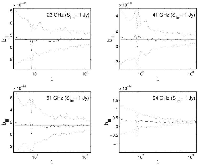
Figure 4: $b_{ps}$ due to a clustered distribution of point sources at four WMAP frequencies: 23, 41, 61 and 94 GHz. As in Figure 3, the straight horizontal line represent the $b_{ps}$ values of Table 1. The dashed line represents the average $b_{ps}$ over 100 simulations and the dotted lines represent the $\pm 1\sigma$ limits.

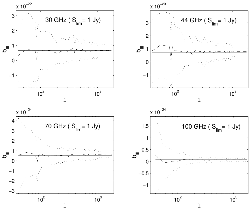
Figure 5: $b_{ps}$ due to a clustered distribution of point sources at Planck LFI frequencies: 30, 44, 70 and 100 GHz. The meaning of the lines is the same as in Figure 4.

On the other hand, to give a preliminary estimate of the $b_{ps}$ at Planck HFI frequencies, we have also calculated the reduced equilateral bispectrum of a non Poisson distribution of sources at 545 GHz. At this frequency the source populations dominating the number counts are dust–enshrouded elliptical galaxies and spheroids at substantial redshift (Toffolatti et al., 1998; Guiderdoni et al., 1998; Granato et al., 2001) and, consequently, the clustering term should not be negligible (Magliocchetti et al., 2001; Perrotta et al., 2003), given that the dilution of the signal is less effective than that of sources showing a broad redshift distribution. The results plotted in Figure 6 are obtained, as before, by distributing sources in the sky using a Poisson distribution which is then modified by the angular correlation functions appropiate for each source populations. As at lower frequencies, the value of $b_{ps}$ estimated by Eq.(15), applied to the simulated maps and with a Poisson distribution of sources, still gives a very good approximation of the value directly obtained by Eq.(10).

As for the correlated distributions, for radio selected ”flat”–spectrum sources, which are giving a quite small but not negligible contribution to the bispectrum at these frequencies, we have still applied the $w(\theta)$ of Loan, Wall and Lahav (1997), under the assumption that the underlying parent population is the same (flat–spectrum QSOs, blazars) up to these frequencies. As for sources whose emission is dominated by cold dust, the lack of direct data at 545 GHz forced us to rely on SCUBA as well as on optical and near–IR surveys (see Perrotta et al. (2003)). By distinguishing the relevant populations in starburts/spirals at low redshift and ellipticals and spheroids at intermediate to high redshift, we then applied to them the $w(\theta)$ of Tegmark et al. (2002) and of Magliocchetti et al. (2001), respectively. This is a very preliminary estimate and, naturally, it will be improved in the next future. Anyway, given that the most relevant quantity is the total number of sources below the detection threshold, the choice of a different – but realistic – angular correlation function does not modify very much the estimated $b_{ps}$: Figure 6 clearly show that the three different evolution models for sources are giving basically the same estimated $b_{ps}$. On the other hand, it is also apparent that at frequencies $\geq 300$ GHz source clustering can greatly enhance the value of $b_{ps}$ and, particularly, at multipoles $\ell\leq$100. This last result is again in agreement with the results of Scott and White (1999); Magliocchetti et al. (2001); Toffolatti et al. (2003) on the angular power spectrum.

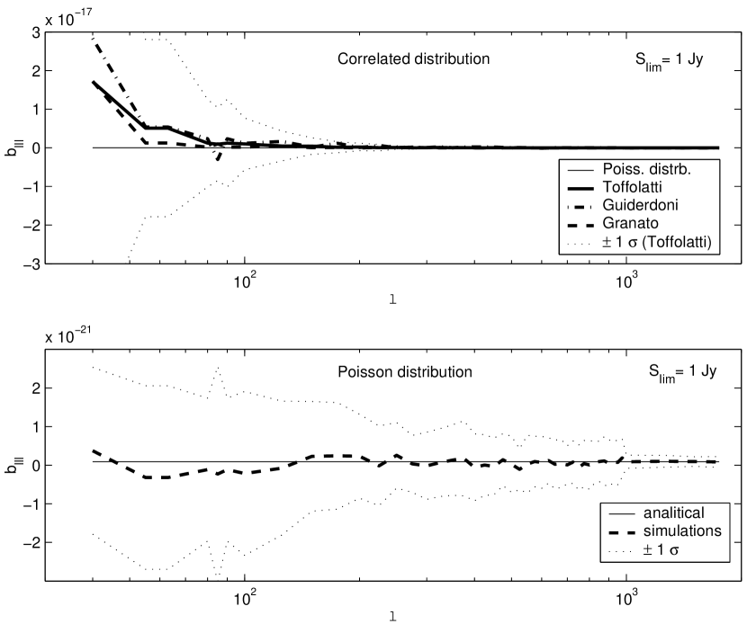
Figure 6: $b_{ps}$ at 545 GHz and applying the conservative source detection limit $S_{lim}=1$ Jy (see text). As in the previous Figures, the straight horizontal line represents the value of Table 1, obtained by Eq.(10): please note that in the two panels the plotted value is the same one, i.e., $b_{ps}=5\times 10^{-23}$, in spite of the great scale difference. The top panel shows the comparison of the average values of $b_{ps}$ obtained by performing 100 simulations with the number counts of three different evolution models (see label on the Figure). We adopted different clustered distribution of sources for each one of the three different models of sources counts (see text). The lower panel displays the comparison of the analytical estimate of $b_{ps}$ with the result of 100 simulations obtained by a simple Poisson distribution of sources (dashed line, TO98 model counts). In the two panels, the dotted lines represent the $\pm 1\sigma$ limits obtained with the TO98 source counts.

4 DISCUSSION AND CONCLUSIONS

The primordial bispectrum is a telling quantity of the non-Gaussianity level of the CMB and its detection should be of great importance for theories of the early Universe. On the other hand, undetected extragalactic sources, which are not Gaussian distributed in the sky are surely giving rise to a bispectrum detectable by current as well as future CMB experiments. In fact, Komatsu et al. (2003) already claimed the first detection of the bispectrum due to undetected point sourecs at 41 GHz by the analysis of the first year WMAP data. Therefore, the possible detection of the primordial CMB bispectrum is severely hampered by the presence of the foreground emission of point sources which has to be carefully evaluated.

Assuming that the sources are Poisson distributed in the sky their reduced bispectrum is easy to calculate by integrating the differential counts of the relevant source populations at a given frequency. In this paper, we have carried out a detailed analysis of the bispectrum due to extragalactic point sources in all Planck and WMAP frequency channels. We used the Toffolatti et al. (1998) evolution model for radio and far–IR selected sources as a template to estimate the $b_{ps}$ foreseen in the case of a Poisson distribution of point sources and by using two different cosmologies (see Section 2). As proved by KS01, the point source bispectrum can be separated from the primordial one taking into account the difference in shape. Our current est imates proves that $b_{ps}$ can be detected in all WMAP channels if the detection limit for sources is $S_{lim}\geq$1 Jy – albeit at the $1\div 2\sigma$ level at 94 GHz – and also in all Planck channels if $S_{lim}\geq$0.1 Jy. Table 1 and Fig. 1, 2 show in detail how the values of $b_{ps}$ of Poisson distributed sources can affect the detection of the primordial bispectrum, $b_{lll}$, in the whole frequency interval around the CMB intensity peak and at Planck LFI frequencies, respectively.

In the case of Poisson distributed sources, our main results can be summarized as follows:

a) the bispectrum detected by Komatsu et al. (2003) in the WMAP 1-year sky maps (Q and V bands) is compatible at the $1\sigma$ level with the predictions on $b_{ps}$ calculated by the number counts of TO98. The best fit value of $b_{ps}$ measured by Komatsu et al. (2003) in the Q band can be explained by undetected extragalactic sources according to the TO98 model predictions multiplied by $\simeq 0.70$, if we integrate the number counts up to $S_{lim}=$0.75 Jy like in Komatsu et al. (2003). On the other hand, in the V band we find a smaller mismatch ($\simeq 0.8\div 0.9$) with current WMAP measurements. Both uncertainties in the measured $b_{ps}$ and errors in TO98 predictions could explain the detected offsets. In particular, the different correction factors which are currently found for the Q and V bands, if confirmed by future analyses, could be indicative that the adopted spectral index distribution of sources has to be partially corrected. Current surveys at 15 and 31 GHz (Waldram et al., 2003; Bennett et al., 2003b) are showing a greater fraction of ”steep”–spectrum radio sources at intermediate to bright fluxes than that foreseen by the original TO98 model. These new results can help in reducing the observed offsets between current measurements of $b_{ps}$ and model predictions while keeping a good fit to the CBI, VSA and WMAP differential source counts. Another, albeit small, source of uncertainty is the underlying cosmology: correction factors of 10-20% in the estimated $b_{ps}$ values are easily introduced in this frequency range by changing $\Omega_{M}$ and $\Omega_{\Lambda}$.

b) The primordial CMB bispectrum, $b_{lll}$, appears higher than $b_{ps}$ only at multipoles close to $\ell\sim 200$ where it reaches its peak value (see Figures 1 and 2). The frequency window inside which the peak value of $b_{lll}$ is detectable sets larger by increasing $f_{nl}$ and by reducing the source detection limit, $S_{lim}$, i.e. it strongly depends on the efficiency of the source detection algorithm. If $f_{nl}=100$ and with $S_{lim}\simeq 0.1$ Jy, the window spans from $\sim 30$ to $\sim 500$ GHz. On the other hand, if $f_{nl}=10$ and $S_{lim}\simeq 2$ Jy, the window shrinks to $100\leq\nu\leq 350$ GHz. These results clearly show that $b_{ps}$ does not hamper the possible detection by Planck of very low values of the coupling parameter ($f_{nl}<10$), comparable to the theoretical limit achievable by the mission.

c) If the detection of $b_{ps}$ is effectively achieved (e.g., by WMAP data) the simple comparison with the $b_{ps}$ levels estimated by the integration of the differential counts of sources, $dN/dS$, allow, in principle, to test the adopted evolution model for sources. Anyway, as already noted by KS01, this can be applied only to the bright end of the number counts, at least for frequencies below 150$\div$200 GHz, given the ‘flat’ slope of the counts – close to or $\beta=2.5$, i.e. ‘euclidean’ – which implies that faint fluxes are not relevant in Eq.(10). As also discussed in Section 2., the adopted cosmology does not affect all the above conclusions.

For estimating to which extent the clustering of sources can affect the value of $b_{ps}$ we have carried out flat 2D simulations in sky patches with pixel sizes of $1.5$ (Planck) and $6$ (WMAP) arcmin. In this analysis we simulated sources with a particular choice of the angular correlation function, but we neglected higher order moments of the distribution. This simplified approach could affect, in principle, the conclusion that source clustering does not modify the bispectrum at frequencies $\leq 100$ GHz (see Figures 3, 4 and 5). However, as discussed in Section 2 and 3, the results are much more determined by the number of undetected sources in the sky (the differential counts of bright sources) than by the choice of the correlation function or by the inclusion of higher order moments in the simulations. We checked that if we apply a different $w(\theta)$ to the same number counts, i.e. to the same evolution model for counts, the estimated $b_{ps}$ keeps practically unchanged.

On the other hand, at frequencies $\nu\geq$300 GHz, the number of sources in the sky at a given flux limit is greatly enhanced by the rising energy spectra due to the emission of the cold dust components. Correspondingly, if sources do cluster down to very low flux limits, the clustering term can dominate the Poisson one and $b_{ps}$ values result greatly enhanced (Figure 6). Therefore, it is surely of great astrophysical interest to study the clustering properties as well as the cosmological evolution of extragalactic sources in this frequency range for obtaining a better assessment of their contribution to the CMB angular power spectrum and bispectrum.

References

- Barreiro et al. (2000) Barreiro, R. B., Hobson, M. P., Lasenby, A. N., Banday, A. J., Gorski K. M., and Hinshaw, G., 2000, MNRAS, 318, 475
- Barreiro et al. (2001) Barreiro, R. B., Martínez-González, E., and Sanz J. L., 2001, MNRAS, 322, 411
- Bennett et al. (2003a) Bennett, C. L., et al., 2003, ApJ, 583, 1
- Bennett et al. (2003b) Bennett, C. L., et al., 2003, ApJ, in press (astro-ph/0302208)
- Bromley and Tegmark (1999) Bromley, B. C., and Tegmark, M., 1999, ApJ, 524, L79
- Cayón et al. (2001) Cayón, L., Sanz, J. L., Martínez-González, E., Banday A. J., Argüeso, F., Gallegos, J. E., Gorski K. M., and Hinshaw G., 2001, MNRAS, 326, 1243
- Cayón et al. (2003) Cayón, L., Martínez-González, E., Argüeso, F., Banday, A. J., and Gorski, K. M., 2003, MNRAS, in press.
- Coble et al. (2003) Coble, K., et al., 2003, ApJ, submitted (astro-ph/0301599)
- Falk et al. (1993) Falk, T., Rangarajan, R., and Srednicki, M. 1993, ApJ, 403, L1
- Ferreira et al. (1998) Ferreira, P. G., Magueijo, J., and Gorski, K.M., 1998, ApJ, 503, L1
- Gangui et al. (1994) Gangui, A., Lucchin, F., Matarrese, S., and Mollerach, S., 1994, ApJ, 430, 447
- Gangui and Martin (2000) Gangui, A., and Martin, J., 2000, Phys. Rev. D, 62, 103004
- González-Nuevo et al. (2003) González-Nuevo, J., Toffolatti, L., and Argüeso, F., 2003, in preparation.
- Gorski et al. (1998) Górski, K.M., Hivon, E., and Wandelt, B.D., 1998, in Evolution of Large Scale Structure: from Recombination to Garching, p.
- Granato et al. (2001) Granato, G. L., Silva, L., Monaco, P., Panuzzo, P., Salucci, P., De Zotti, G., and Danese, L., 2001, MNRAS, 324, 757
- Guiderdoni et al. (1998) Guiderdoni, B., Hivon, E., Bouchet, F., and Maffei, B., 1998, MNRAS, 295, 877
- Hinshaw et al. (2003) Hinshaw, G., et al., 2003, ApJ, submitted (astro-ph/0302217)
- Kofman et al. (1991) Kofman, L., Blumenthal, G. R., Hodges, H., and, Primack J. R., 1991, in Large-Scale structures and peculiar Motions in the Universe, edited by Latham, D. W.& da Costa, L. N., ASP Conference Series, Vol.15, p.339
- Komatsu and Spergel (2001) Komatsu, E., and Spergel, D. N., 2001, Phys. Rev. D, 63, 063002
- Komatsu et al. (2002) Komatsu, E., Wandelt, B. D., Spergel, D. N., Banday, A. J., and Gorski, K. M., 2002, ApJ, 566, 199
- Komatsu et al. (2003) Komatsu, E., Kogut, A., Nolta, M. R., Bennett, C. L., Halpern, M., Hinshaw, G., Jarosik, N., Limon, M., Meyer, S. S., Page, L., Spergel, D. N., Tucker, G. S., Verde, L., Wollack, E., and Wright, E. L., the WMAP team, 2003, ApJ, in press (astro-ph/0302223)
- Loan, Wall and Lahav (1997) Loan, A. J., Wall, J. V. & Lahav, O., 1997, MNRAS, 286, 994
- Luo (1994) Luo, X. 1994, ApJ, 427, L71
- Magliocchetti et al. (2001) Magliocchetti, M., Moscardini, L., Panuzzo, P., Granato, G.L., De Zotti, G., and Danese, L., 2001, MNRAS, 325, 1553
- Mandolesi et al. (1998) Mandolesi, N., et al., 1998, proposal submitted to ESA for the ”Planck” Low Frequency Instrument (LFI)
- Mason et al. (2003) Mason, B.S., et al., 2003, ApJ, in press, (astro-ph/0205384)
- Pando et al. (1998) Pando, J., Valls-Gabaud, D., and Fang, L. Z., 1998, Phys. Rev. Lett., 81, 4568
- Park, Park and Ratra (2002) Park, C. G., Park, C., and Ratra, B., 2002, ApJ, 568, 9
- Perrotta et al. (2003) Perrotta, F., Magliocchetti, M., Baccigalupi, C., Bartelmann, M., De Zotti, G., Granato, G.L., Silva, L., and Danese, L., 2002, MNRAS, 338, 623
- Polenta et al. (2002) Polenta, G., et al., 2002, ApJ, 572, L27.
- Puget et al. (1998) Puget, J.-L., et al., 1998, proposal submitted to ESA for the ”Planck” High Frequency Instrument (HFI)
- Pyne and Carroll (1996) Pyne, T., and Carroll, S.M., 1996, Phys. Rev. D, 53, 2920
- Salopek and Bond (1990) Salopek, D. S., and Bond, J. R., Phys. Rev. D, 42, 3936
- Santos et al. (2002) Santos, M. G., et al., 2002, Phys. Rev. Lett., 88, 241602
- Scott and White (1999) Scott, D., and White, M., 1999, Astronomy & Astrophysics, 346, 1
- Schmalzing and Gorski (1997) Schmalzing, J., and Gorski, K. M., 1997, MNRAS, 297, 355
- Sokasian, Gawiser and Smoot (2001) Sokasian, A., Gawiser, E., and Smoot, G. F., 2001, ApJ, 562, 88
- Spergel et al. (2003) Spergel, D. N., Komatsu, E., Kogut, A., Bennett, C. L., Halpern, M., Hinshaw, G., Jarosik, N., Limon, M., Meyer, S. S., Page, L., Nolta, M. R., Tucker, G. S., Verde, L., Wollack, E., and Wright, E. L., the WMAP team, 2003, ApJ, submitted (astro-ph/0302209)
- Taylor et al. (2001) Taylor, A. C., Grainge, K., Jones, M. E., Pooley, G. G., Saunders, R. D. E., and Waldram, E. M., 2001, MNRAS, 327, L1
- Taylor et al. (2003) Taylor, A. C., et al., 2003, MNRAS, in press, (astro-ph/0205381)
- Toffolatti et al. (1998) Toffolatti, L., Argüeso Gómez, F., de Zotti, G., Mazzei, P., Franceschini, A., Danese, L. and Burigana, C., 1998, MNRAS, 297, 117
- Toffolatti et al. (1999) Toffolatti, L., Argüeso, F., De Zotti, G., and Burigana, C., 1999, in ASP Conf. Series Vol. 181, Microwave Foregrounds, A. de Oliveira-Costa and M. Tegmark eds., p.153
- Toffolatti et al. (2003) Toffolatti, L., González-Nuevo, J., and Argüeso, F., 2003, in preparation.
- Vielva et al. (2003) Vielva, P., Martínez-González E., Gallegos, J. E., Toffolatti, L., and Sanz, J.L., 2003, MNRAS, in press (astro-ph/0212578)
- Waldram et al. (2003) Waldram, E., Pooley, G.G., Grainge, K.J.B., Jones, M.E., Saunders, R.D.E., Scott, P.F., and Taylor, A., 2003, MNRAS, in press (astro-ph/0304275)
- Wang and Kamionkowski (2000) Wang, L., and Kamionkowski, M. 2000, Phys. Rev. D, 61, 63504
- Wu et al. (2001) Wu, J. H. P., Balbi, A., Borrill, J., Ferreira, P. G., Hanany, S., Jaffe, A. H., Lee, A. T., Oh, S., Rabii, B., Richards, P. L., Smoot, G., Stompor, R., and Winant, C.D., 2001, ApJS, 132, 1.