The Rest-Frame Optical Luminosity Density, Color, and Stellar Mass Density of the Universe from z=0 to z=3

Abstract

We present the evolution of the rest-frame optical luminosity density, $j^{\rm rest}_{\lambda}$, of the integrated rest-frame optical color, and of the stellar mass density, $\rho_{*}$, for a sample of $K_{s}$-band selected galaxies in the HDF-S. We derived $j^{\rm rest}_{\lambda}$ in the rest-frame $U$, $B$, and $V$-bands and found that $j^{\rm rest}_{\lambda}$ increases by a factor of $1.9\pm 0.4$, $2.9\pm 0.6$, and $4.9\pm 1.0$ in the $V$, $B$, and $U$ rest-frame bands respectively between a redshift of 0.1 and 3.2. We derived the luminosity weighted mean cosmic $(U~{}-~{}B)_{rest}$ and $(B~{}-~{}V)_{rest}$ colors as a function of redshift. The colors bluen almost monotonically with increasing redshift; at $z=0.1$, the $(U~{}-~{}B)_{rest}$ and $(B~{}-~{}V)_{rest}$ colors are 0.16 and 0.75 respectively, while at $z=2.8$ they are -0.39 and 0.29 respectively. We derived the luminosity weighted mean ${\rm M}/{\rm L}^{*}_{V}$ using the correlation between $(U~{}-~{}V)_{rest}$ and log₁₀${\rm M}/{\rm L}^{*}_{V}$ which exists for a range in smooth SFHs and moderate extinctions. We have shown that the mean of individual ${\rm M}/{\rm L}^{*}_{V}$ estimates can overpredict the true value by $\sim 70\%$ while our method overpredicts the true values by only $\sim 35\%$. We find that the universe at $z\sim 3$ had $\sim 10$ times lower stellar mass density than it does today in galaxies with ${\rm L}_{\rm V}^{rest}$ $>1.4\times 10^{10}$${\rm~{}h_{70}^{-2}~{}L_{\odot}}$. 50% of the stellar mass of the universe was formed by $z\sim 1-1.5$. The rate of increase in $\rho_{*}$ with decreasing redshift is similar to but above that for independent estimates from the HDF-N, but is slightly less than that predicted by the integral of the SFR($z$) curve.

1. Introduction

A primary goal of galaxy evolution studies is to elucidate how the stellar content of the present universe was assembled over time. Enormous progress has been made in this field over the past decade, driven by advances over three different redshift ranges. Large scale redshift surveys with median redshifts of $z\sim 0.1$ such as the Sloan Digital Sky Survey (SDSS; York et al. 2000) and the 2dF Galaxy Redshift Survey (2dFGRS; Colless et al. 2001), coupled with the near infrared (NIR) photometry from the 2 Micron All Sky Survey (2MASS; Skrutskie et al. 1997), have recently been able to assemble the complete samples, with significant co-moving volumes, necessary to establish crucial local reference points for the local luminosity function (e.g. Folkes et al. 1999; Blanton et al. 2001; Norberg et al. 2002; Blanton et al. 2003c) and the local stellar mass function of galaxies (Cole et al., 2001; Bell et al., 2003a).

At $z\lesssim 1$, the pioneering study of galaxy evolution was the Canada France Redshift Survey (CFRS; Lilly et al. 1996). The strength of this survey lay not only in the large numbers of galaxies with confirmed spectroscopic redshifts, but also in the $I$-band selection, which enabled galaxies at $z\lesssim 1$ to be selected in the rest-frame optical, the same way in which galaxies are selected in the local universe.

At high redshifts the field was revolutionized by the identification, and subsequent detailed follow-up, of a large population of star-forming galaxies at $z>2$ (Steidel et al., 1996). These Lyman Break Galaxies (LBGs) are identified by the signature of the redshifted break in the far UV continuum caused by intervening and intrinsic neutral hydrogen absorption. There are over 1000 spectroscopically confirmed LBGs at $z>2$, together with the analogous U-dropout galaxies identified using Hubble Space Telescope (HST) filters. The individual properties of LBGs have been studied in great detail. Estimates for their star formation rates (SFRs), extinctions, ages, and stellar masses have been estimated by modeling the broad band fluxes (Sawicki & Yee 1998; hereafter SY98; Papovich et al. 2001; hereafter P01; Shapley et al. 2001). Independent measures of their kinematic masses, metallicities, SFRs, and initial mass functions (IMFs) have been determined using rest-frame UV and optical spectroscopy (Pettini et al., 2000; Shapley et al., 2001; Pettini et al., 2001, 2002; Erb et al., 2003).

Despite these advances, it has proven difficult to reconcile the ages, SFRs, and stellar masses of individual galaxies at different redshifts within a single galaxy formation scenario. Low redshift studies of the fundamental plane indicate that the stars in elliptical galaxies must have been formed by $z>2$ (e.g., van Dokkum et al. 2001) and observations of evolved galaxies at $1<z<2$ indicate that the present population of elliptical galaxies was already in place at $z\gtrsim 2.5$ (e.g., Benítez et al. 1999; Cimatti et al. 2002; but see Zepf 1997). In contrast, studies of star forming Lyman Break Galaxies spectroscopically confirmed to lie at $z>2$ (LBGs; Steidel et al. 1996, 1999) claim that LBGs are uniformly very young and a factor of 10 less massive than present day ${\rm L}_{*}$ galaxies (e.g., SY98; P01; Shapley et al. 2001).

An alternative method of tracking the build-up of the cosmic stellar mass is to measure the total emissivity of all relatively unobscured stars in the universe, thus effectively making a luminosity weighted mean of the galaxy population. This can be partly accomplished by measuring the evolution in the global luminosity density $j(z)$ from galaxy redshift surveys. Early studies at intermediate redshift have shown that the rest-frame UV and $B$-band $j(z)$ are steeply increasing out to $z\sim 1$ (e.g., Lilly et al. 1996; Fried et al. 2001). Wolf et al. (2003) has recently measured $j(z)$ at $0<z<1.2$ from the COMBO-17 survey using $\sim$25,000 galaxies with redshifts accurate to $\sim 0.03$ and a total area of 0.78 degrees. At rest-frame 2800${\rm\AA}$ these measurements confirm those of Lilly et al. (1996) but do not support claims for a shallower increase with redshift which goes like $(1+z)^{1.5}$ as claimed by Cowie, Songaila, & Barger (1999) and Wilson et al. (2002). On the other hand, the $B$-band evolution from Wolf et al. (2003) is only a factor of $\sim 1.6$ between $0<z<1$, considerably shallower than the factor of $\sim 3.75$ increase seen by Lilly et al. (1996). At $z>2$ measurements of the rest-frame UV $j(z)$ have been made using the optically selected LBG samples (e.g., Madau et al. 1996; Sawicki, Lin, & Yee 1997; Steidel et al. 1999; Poli et al. 2001) and NIR selected samples (Kashikawa et al., 2003; Poli et al., 2003; Thompson, 2003) and, with modest extinction corrections, the most recent estimates generically yield rest-frame UV $j(z)$ curves which, at $z>2$, are approximately flat out to $z\sim 6$ (cf. Lanzetta et al. 2002). Dickinson et al. (2003; hereafter D03) have used deep NIR data from NICMOS in the HDF-N to measure the rest-frame $B$-band luminosity density out to $z\sim 3$, finding that it remained constant to within a factor of $\sim 3$. By combining $j(z)$ measurements at different rest-frame wavelengths and redshifts, Madau, Pozzetti, & Dickinson (1998) and Pei, Fall, & Hauser (1999) modeled the emission in all bands using an assumed global SFH and used it to constrain the mean extinction, metallicity, and IMF. Bolzonella, Pelló, & Maccagni (2002) measured NIR luminosity functions in the HDF-N and HDF-S and find little evolution in the bright end of the galaxy population and no decline in the rest-frame NIR luminosity density out to $z\sim 2$. In addition, Baldry et al. (2002) and Glazebrook et al. (2003a) have used the mean optical cosmic spectrum at $z\sim 0$ from the 2dFGRS and the SDSS respectively to constrain the cosmic star formation history.

Despite the wealth of information obtained from studies of the integrated galaxy population, there are major difficulties in using these many disparate measurements to re-construct the evolution in the stellar mass density. First, and perhaps most important, the selection criteria for the low and high redshift surveys are usually vastly different. At $z<1$ galaxies are selected by their rest-frame optical light. At $z>2$, however, the dearth of deep, wide-field NIR imaging has forced galaxy selection by the rest-frame UV light. Observations in the rest-frame UV are much more sensitive to the presence of young stars and extinction than observations in the rest-frame optical. Second, state-of-the-art deep surveys have only been performed in small fields and the effects of field-to-field variance at faint magnitudes, and in the rest-frame optical, are not well understood.

In the face of field-to-field variance, the globally averaged rest-frame color may be a more robust characterization of the galaxy population than either the luminosity density or the mass density because it is, to the first order, insensitive to the exact density normalization. At the same time, it encodes information about the dust obscuration, metallicity, and SFH of the cosmic stellar population. It therefore provides an important constraint on galaxy formation models which may be reliably determined from relatively small fields.

To track consistently the globally averaged evolution of the galaxies which dominate the stellar mass budget of the universe – as opposed to the UV luminosity budget – over a large redshift range a different strategy than UV selection must be adopted. It is not only desirable to measure $j(z)$ in a constant rest-frame optical bandpass, but it is also necessary that galaxies be selected by light redward of the Balmer/4000${\rm\AA}$ break, where the light from older stars contributes significantly to the SED. To accomplish this, we obtained ultra-deep NIR imaging of the WFPC2 field of the HDF-S (Casertano et al., 2000) with the Infrared Spectrograph And Array Camera (ISAAC; Moorwood et al. 1997) at the Very Large Telescope (VLT) as part of the Faint Infrared Extragalactic Survey (FIRES; Franx et al. 2000). The FIRES data on the HDF-S, detailed in Labbé et al. (2003; hereafter L03), provide us with the deepest ground-based $J_{s}$ and $H$ data and the overall deepest $K_{s}$-band data in any field allowing us to reach rest-frame optical luminosities in the $V$-band of $\sim 0.6$ ${\rm L}_{*}^{\rm local}$ at $z\sim 3$. First results using a smaller set of the data were presented in Rudnick et al. (2001; hereafter R01). The second FIRES field, centered on the $z=0.83$ cluster MS1054-03, has $\sim 1$ magnitude less depth but $\sim 5$ times greater area (Förster Schreiber et al., 2003).

In the present work we will draw on photometric redshift estimates, $z_{phot}$ for the $K_{s}$-band selected sample in the HDF-S (R01; L03), and on the observed SEDs, to derived rest-frame optical luminosities ${\rm L^{rest}_{\lambda}}$ for a sample of galaxies selected by light redder than the rest-frame optical out to $z\sim 3$. In § 2 we describe the observations, data reduction, and the construction of a $K_{s}$-band selected catalog with $0.3-2.2\mu m$ photometry, which selects galaxies at $z<4$ by light redward of the 4000${\rm\AA}$ break. In § 3 we describe our photometric redshift technique, how we estimate the associated uncertainties in $z_{phot}$, and how we measure ${\rm L^{rest}_{\lambda}}$ for our galaxies. In § 4 we use our measures of ${\rm L^{rest}_{\lambda}}$ for the individual galaxies to derive the mean cosmic luminosity density, $j^{\rm rest}_{\lambda}$ and the cosmic color and then use these to measure the stellar mass density $\rho_{*}$ as a function of cosmic time. We discuss our results in § 5 and summarize in § 6. Throughout this paper we assume $\Omega_{\mathrm{M}}=0.3,~{}\Omega_{\Lambda}=0.7,~{}\mathrm{and~{}H_{o}}=70~{}{\rm h_{70}~{}km~{}s^{-1}Mpc^{-1}}$ unless explicitly stated otherwise.

2. Data

A complete description of the FIRES observations, reduction procedures, and the construction of photometric catalogs is presented in detail in L03; we outline the important steps below.

Objects were detected in the $K_{s}$-band image with version 2.2.2 of the SExtractor software (Bertin & Arnouts, 1996). For consistent photometry between the space and ground-based data, all images were then convolved to $0\farcs 48$, the seeing in our worst NIR band. Photometry was then performed in the $U_{300}$, $B_{450}$, $V_{606}$, $I_{814}$, $J_{s}$, $H$, and $K_{s}$-band images using specially tailored isophotal apertures defined from the detection image. In addition, a measurement of the total flux in the $K_{s}$-band, $K_{s,{\rm AB}}^{\rm tot}$, was obtained using an aperture based on the SExtractor AUTO aperture. Our effective area is 4.74 square arcminutes, including only areas of the chip which were well exposed. All magnitudes are quoted in the Vega system unless specifically noted otherwise. Our adopted conversions from Vega system to the AB system are $J_{s,vega}$ = $J_{s,{\rm AB}}$ - 0.90, $H_{vega}$ = $H_{{\rm AB}}$ - 1.38, and $K_{s,vega}$ = $K_{s,{\rm AB}}$ - 1.86 (Bessell & Brett, 1988).

3. Measuring Photometric Redshifts and Rest-Frame Luminosities

3.1. Photometric Redshift Technique

We estimated $z_{phot}$ from the broad-band SED using the method described in R01, which attempts to fit the observed SED with a linear combination of redshifted galaxy templates. We made two modifications to the R01 method. First, we added an additional template constructed from a 10 Myr old, single age, solar metallicity population with a Salpeter (1955) initial mass function (IMF) based on empirical stellar spectra from the 1999 version of the Bruzual & Charlot (1993) stellar population synthesis code. Second, a 5% minimum flux error was adopted for all bands to account for the night-to-night uncertainty in the derived zeropoints and for template mismatch effects, although in reality both of these errors are non-gaussian.

Using 39 galaxies with reliable FIRES photometry and spectroscopy available from Cristiani et al. (2000), Rigopoulou et al. (2000), Glazebrook (2003b), Vanzella et al. (2002), and Rudnick et al. (2003) we measured the redshift accuracy  of our technique to be $\left\langle~{}|z_{spec}-z_{phot}|~{}/~{}(1+z_{spec})~{}\right\rangle=0.09$ for $z<3$ . There is one galaxy at $z_{spec}$ =2.025 with $z_{phot}$ $=0.12$ but with a very large internal $z_{phot}$ uncertainty. When this object is removed, $\left\langle~{}|z_{spec}-z_{phot}|~{}/~{}(1+z_{spec})~{}\right\rangle=0.05$ at $z_{spec}$ $>1.3$.

For a given galaxy, the photometric redshift probability distribution can be highly non-Gaussian and contain multiple $\chi^{2}$ minima at vastly different redshifts. An accurate estimate of the error in $z_{phot}$ must therefore not only contain the two-sided confidence interval in the local $\chi^{2}$ minimum, but also reflect the presence of alternate redshift solutions. The difficulties of measuring the uncertainty in $z_{phot}$ were discussed in R01 and will not be repeated in detail here. To improve on R01, however, we have developed a Monte Carlo method which takes into account, on a galaxy-by-galaxy basis, flux errors and template mismatch. These uncertainty estimates are called $\delta z_{phot}$. For a full discussion of this method see Appendix A.

Galaxies with $K_{s,{\rm AB}}^{\rm tot}$ $\geq 25$ have such high photometric errors that the $z_{phot}$ estimates can be very uncertain. At $K_{s,{\rm AB}}^{\rm tot}$ $<25$, however, objects are detected at better than the 10-sigma level and have well measured NIR SEDs, important for locating redshifted optical breaks. For this reason, we limited our catalog to the 329 objects that have $K_{s,{\rm AB}}^{\rm tot}$ $<25$, lie on well exposed sections of the chip, and are not identified as stars (see §3.1.1).

3.1.1 Star Identification

To identify probable stars in our catalog we did not use the profiles measured from the WFPC2-imaging because it is difficult to determine the size at faint levels. At the same time, we verified that the stellar template fitting technique identified all bright unsaturated stars in the image. Instead, we compared the observed SEDs with those from 135 NextGen version 5.0 stellar atmosphere models described in Hauschildt, Allard, & Baron (1999) and available at http://dilbert.physast.uga.edu/$\sim$yeti/mdwarfs.html. We used models with log$(g)$ of 5.5 and 6, effective temperatures ranging from 1600 K to 10,000 K, and metallicities of solar and 1/10th solar. We identified an object as a stellar candidate if the raw $\chi^{2}$ of the stellar fit was lower than that of the best-fit galaxy template combination. Four of the stellar candidates from this technique (objects 155, 230, 296, and 323) are obviously extended and were excluded from the list of stellar candidates. Two bright stars (objects 39 and 51) were not not identified by this technique because they are saturated in the HST images and were added to the list by hand. We ended up with a list of 29 stars that had $K_{s,{\rm AB}}^{\rm tot}$ $<25$ and lie on well exposed sections of the chip. These were excluded from all further analysis.

3.2. Rest-Frame Luminosities

To measure the ${\rm L^{rest}_{\lambda}}$ of a galaxy one must combine its redshift with the observed SED to estimate the intrinsic SED. In practice, this requires some assumptions about the intrinsic SED.

In R01 we derived rest-frame luminosities from the best-fit combination of spectral templates at $z_{phot}$, which assumes that the intrinsic SED is well modeled by our template set. We know that for many galaxies the best-fit template matches the position and strength of the spectral breaks and the general shape of the SED. There are, however, galaxies in our sample which show clear residuals from the best fit template combination. Even for the qualitatively good fits, the model and observed flux points can differ by $\sim 10\%$, corresponding to a $\sim 15\%$ error in the derived rest-frame color. As we will see in §4.2, such color errors can cause errors of up to a factor of 1.5 in the $V$-band stellar mass-to-light ratio, ${\rm M}/{\rm L}^{*}_{V}$.

Here we used a method of estimating ${\rm L^{rest}_{\lambda}}$ which does not depend directly on template fits to the data but, rather, interpolates directly between the observed bands using the templates as a guide. We define our rest-frame photometric system in Appendix B and explain our method for estimating ${\rm L^{rest}_{\lambda}}$ in Appendix C.

We plot in Figure 1 the rest-frame luminosities vs. redshift and enclosed volume for the $K_{s,{\rm AB}}^{\rm tot}$ $<25$ galaxies in the FIRES sample. The different symbols represent different $\delta z_{phot}$ values and since the derived luminosity is tightly coupled to the redshift, we do not independently plot ${\rm L^{rest}_{\lambda}}$ errorbars. The tracks indicate the ${\rm L^{rest}_{\lambda}}$ for different SED types normalized to $K_{s,{\rm AB}}^{\rm tot}$ $=25$, while the intersection of the tracks in each panel indicates the redshift at which the rest-frame filter passes through our $K_{s}$-band detection filter. There is a wide range in ${\rm L^{rest}_{\lambda}}$ at all redshifts and there are galaxies at $z>2$ with ${\rm L^{rest}_{\lambda}}$ much in excess of the local ${\rm L}_{*}$ values. Using the full FIRES dataset, we are much more sensitive than in R01; objects at $z\approx 3$ with $K_{s,{\rm AB}}^{\rm tot}$ $=25$ have ${\rm L}_{\rm V}^{rest}$ $\approx 0.6*$${\rm L}_{*,V}^{\rm local}$, as defined from the z=0.1 sample of Blanton et al. (2003c; hereafter B03). As seen in R01 there are many galaxies at $z>2$, in all bands, with ${\rm L^{rest}_{\lambda}}$ $\geq$${\rm L}_{*}^{\rm local}$. R01 found 10 galaxies at $2\leq z\leq 3.5$ with ${\rm L}_{\rm B}^{rest}$ $>10^{11}$${\rm~{}h_{70}^{-2}~{}L_{\odot}}$ and inferred a brightening in the luminosity function of $\sim 1-1.3$ magnitudes. We confirm their result when using the same local luminosity function (Blanton et al., 2001). Although this brightening is biased upwards by photometric redshift errors, we find a similar brightening of approximately $\sim 1$ magnitude after correction for this effect. As also noticed in R01, we found a deficit of luminous galaxies at $1.5\lesssim z\lesssim 2$ although this deficit is not as pronounced at lower values of ${\rm L^{rest}_{\lambda}}$. The photometric redshifts in the HDF-S, however, are not well tested in this regime. To help judge the reality of this deficit we compared our photometric redshifts on an object-by-object basis to those of the Rome group (Fontana et al., 2000) who derived $z_{phot}$ estimates for galaxies in the HDF-S using much shallower NIR data. We find generally good agreement in the $z_{phot}$ estimates, although there is a large scatter at $1.5<z<2.0$. Both sets of photometric redshifts show a deficit in the $z_{phot}$ distribution, although the Rome group’s gap is less pronounced than ours and is at a slightly lower redshift. In addition, we examined the photometric redshift distribution of the NIR selected galaxies of D03 in the HDF-N, which have very deep NIR data. These galaxies also showed a gap in the $z_{phot}$ distribution at $z\sim 1.6$. Together these results indicate that systematic effects in the $z_{phot}$ determinations may be significant at $1.5<z<2.0$. On the other hand, we also derived photometric redshifts for a preliminary set of data in the MS1054-03 field of the FIRES survey, whose filter set is similar, but which has a $U$ instead of $U_{300}$ filter. In this field, no systematic depletion of $1.5<z<2$ galaxies was found. It is therefore not clear what role systematic effects play in comparison to field-to-field variations in the true redshift distribution over this redshift range. Obtaining spectroscopic redshifts at $1.5<z<2$ is the only way to judge the accuracy of the $z_{phot}$ estimates in this regime.

We have also split the points up according to whether or not they satisfied the U-dropout criteria of Giavalisco & Dickinson (2001) which were designed to pick unobscured star-forming galaxies at $z\gtrsim 2$. As expected from the high efficiency of the U-dropout technique, we find that only 15% of the 57 classified U-dropouts have $z_{phot}$ $<2$. As we will discuss in §4.1 we measured the luminosity density for objects with ${\rm L}_{\rm V}^{rest}$ $>1.4\times 10^{10}$${\rm~{}h_{70}^{-2}~{}L_{\odot}}$. Above this threshold, there are 62 galaxies with $2<z<3.2$, of which 26 are not classified as U-dropouts. These non U-dropouts number among the most rest-frame optically luminous galaxies in our sample. In fact, the most rest-frame optically luminous object at $z<3.2$ (object 611) is a galaxy which fails the U-dropout criteria. 10 of these 26 objects, including object 611, also have $J-K>2.3$, a color threshold which has been shown by Franx et al. (2003) and van Dokkum et al. (2003) to efficiently select galaxies at $z>2$. These galaxies are not only luminous but also have red rest-frame optical colors, implying high ${\rm M}/{\rm L}^{*}$ values. Franx et al. (2003) showed that they likely contribute significantly ($\sim 43\%$) to the stellar mass budget at high redshifts.

3.2.1 Emission Lines

There will be emission line contamination of the rest-frame broad-band luminosities when rest-frame optical emission lines contribute significantly to the flux in our observed filters. P01 estimated the effect of emission lines in the NICMOS F160W filter and the $K_{s}$ filter and found that redshifted, rest-frame optical emission lines, whose equivalent widths are at the maximum end of those observed for starburst galaxies (rest-frame equivalent width $\sim 200$${\rm\AA}$), can contribute up to 0.2 magnitudes in the NIR filters. In addition, models of emission lines from Charlot & Longhetti (2001) show that emission lines will tend to drive the $(U~{}-~{}B)_{rest}$ color to the blue more easily than the $(B~{}-~{}V)_{rest}$ color for a large range of models. Using the $UBV$ photometry and spectra of nearby galaxies from the Nearby Field Galaxy Survey (NFGS; Jansen et al. 2000a; Jansen et al. 2000b) we computed the actual correction to the $(U~{}-~{}B)_{rest}$ and $(B~{}-~{}V)_{rest}$ colors as a function of $(B~{}-~{}V)_{rest}$. For the bluest galaxies in $(B~{}-~{}V)_{rest}$, emission lines bluen the $(U~{}-~{}B)_{rest}$ colors by $\sim 0.05$ and the $(B~{}-~{}V)_{rest}$ colors only by $<0.01$. Without knowing beforehand the strength of emission lines in any of our galaxies, we corrected our rest-frame colors based on the results from Jansen et al. We ignored the very small correction to the $(B~{}-~{}V)_{rest}$ colors and corrected the $(U~{}-~{}B)_{rest}$ colors using the equation:

$$(U-B)_{corrected}=(U-B)-0.0658\times(B-V)+0.0656$$ (1)

which corresponds to a linear fit to the NFGS data. These effects might be greater for objects with strong AGN contribution to their fluxes.

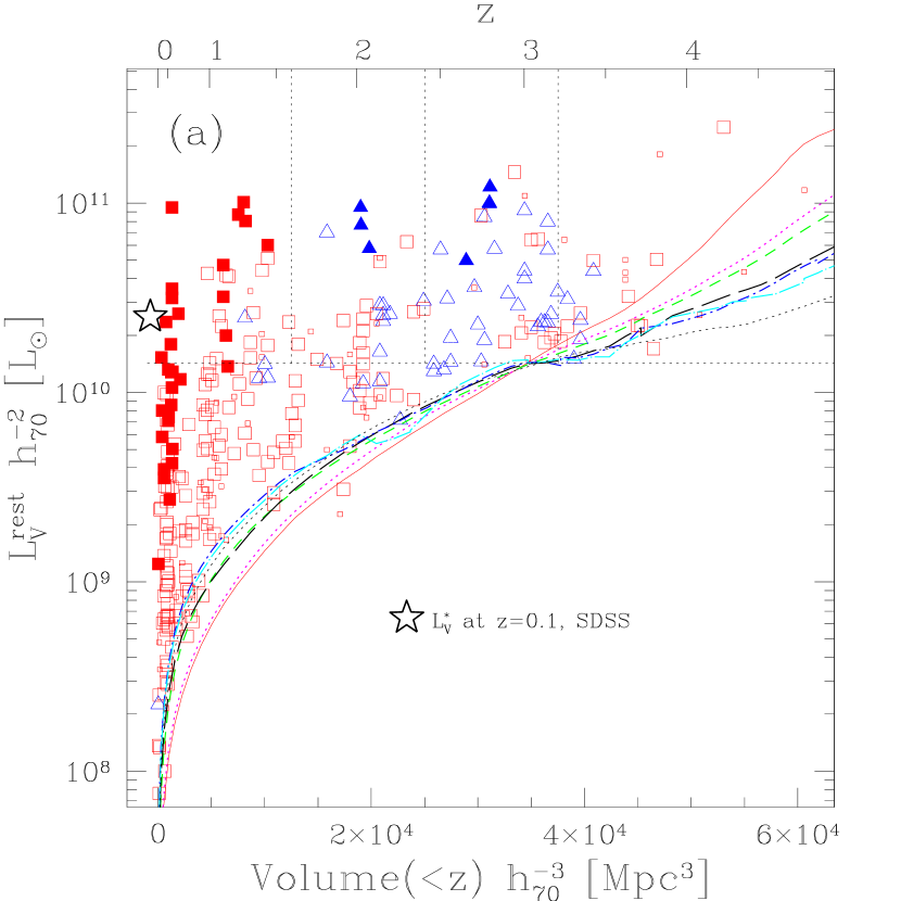
Figure 1.— The distribution of rest-frame $V$, $B$, and $U$-band luminosities as a function of enclosed co-moving volume and $z_{phot}$ is shown in figures (a), (b), and (c) respectively for galaxies with $K_{s,{\rm AB}}^{\rm tot}$ $<25$. Galaxies which have spectroscopic redshifts are represented by solid points and for these objects ${\rm L^{rest}_{\lambda}}$ is measured at $z_{spec}$. Large symbols have $\delta z_{phot}/(1+z_{phot})<0.16$ and small symbols have $\delta z_{phot}/(1+z_{phot})\geq 0.16$. Triangle points would be classified as U-dropouts according to the selection of Giavalisco & Dickinson (2001). As is expected, most of the galaxies selected as U-dropouts have $z_{phot}$ $\gtrsim 2$. Note, however, the large numbers of rest-frame optically luminous galaxies at $z>2$ which would not be selected as U-dropouts. The large stars in each panel indicate the value of ${\rm L}_{*}^{\rm local}$ from Blanton et al. (2003c). In the $V$-band we are sensitive to galaxies at 60% of ${\rm L}_{*}^{\rm local}$ even at $z\sim 3$ and there are galaxies at $z_{phot}$ $\geq 2$ with ${\rm L^{rest}_{\lambda}}$ $\geq 10^{11}$${\rm~{}h_{70}^{-2}~{}L_{\odot}}$. The tracks represent the values of ${\rm L^{rest}_{\lambda}}$ for our seven template spectra normalized at each redshift to $K_{s,{\rm AB}}^{\rm tot}$ $=25$. The specific tracks correspond to the E (solid), Sbc (dot), Scd (short dash), Im (long dash), SB1 (dot–short dash), SB2 (dot–long dash), and 10my (dot) templates. The horizontal dotted line in (a) indicates the luminosity threshold ${\rm L}_{V}^{\rm thresh}$ above which we measure the rest-frame luminosity density $j^{\rm rest}_{\lambda}$ and the vertical dotted lines in each panel mark the redshift boundaries of the regions for which we measure $j^{\rm rest}_{\lambda}$.

4. The Properties of the Massive Galaxy Population

In this section we discuss the use of the $z_{phot}$ and ${\rm L^{rest}_{\lambda}}$ estimates to derive the integrated properties of the population, namely the luminosity density, the mean cosmic rest-frame color, the stellar mass-to-light ratio ${\rm M}/{\rm L}^{*}$, and the stellar mass density $\rho_{*}$. As will be described below, addressing the integrated properties of the population reduces many of the uncertainties associated with modeling individual galaxies and, in the case of the cosmic color, is less sensitive to field-to-field variations.

4.1. The Luminosity Density

Using our ${\rm L^{rest}_{\lambda}}$ estimates from the $K_{s,{\rm AB}}^{\rm tot}$ $<25$ galaxies (see §3.2), we traced the redshift evolution of the rest-frame optically most luminous, and therefore presumably most massive, galaxies by measuring the rest-frame luminosity density $j^{\rm rest}_{\lambda}$ of the visible stars associated with them. The results are presented in Table 1 and plotted against redshift and elapsed cosmic time in Figure 2. As our best alternative to a selection by galaxy mass, we selected our galaxies in our reddest rest-frame band available at $z\sim 3$, i.e. the $V$-band. In choosing the $z$ and ${\rm L^{rest}_{\lambda}}$ regime over which we measured $j^{\rm rest}_{\lambda}$ we wanted to push to as high of a redshift as possible with the double constraint that the redshifted rest-frame filter still overlapped with the $K_{s}$ filter and that we were equally complete at all considered redshifts. By choosing an ${\rm L}_{\rm V}^{rest}$ threshold, ${\rm L}_{V}^{\rm thresh}$ $=1.4\times 10^{10}$${\rm~{}h_{70}^{-2}~{}L_{\odot}}$, and a maximum redshift of $z=3.2$, we could select galaxies down to 0.6 ${\rm L}_{*,V}^{\rm local}$ with constant efficiency regardless of SED type. We then divided the range out to $z=3.2$ into three bins of equal co-moving volume which correspond to the redshift intervals 0–1.6, 1.6–2.41, and 2.41–3.2.

In a given redshift interval, we estimated $j^{\rm rest}_{\lambda}$ directly from the data in two steps. We first added up all the luminosities of galaxies which satisfied our ${\rm L}_{V}^{\rm thresh}$ criteria defined above and which had $\delta z_{phot}$ $/(1+z_{phot})\leq 0.16$, roughly twice the mean disagreement between $z_{phot}$ and $z_{spec}$ (see §3.1). Galaxies rejected by our $\delta z_{phot}$ cut but with ${\rm L}_{\rm V}^{rest}$ $>$${\rm L}_{V}^{\rm thresh}$, however, contribute to the total luminosity although they are not included in this first estimate. Under the assumption that these galaxies are drawn from the same luminosity function as those which passed the $\delta z_{phot}$ cut, we computed the total luminosity, including the light from the $n_{acc}$ accepted galaxies and the light lost from the $n_{rej}$ rejected galaxies as

$${\rm L_{tot}}={\rm L_{meas}}\times(1+\frac{n_{rej}}{n_{acc}}).$$ (2)

As a test of the underlying assumption of this correction we performed a K-S test on the distributions of $K_{s}$ magnitudes for the rejected and accepted galaxies in each of our three volume bins. In all three redshift bins, the rejected galaxies have $K_{s,{\rm AB}}^{\rm tot}$ distributions which are consistent at the $>90\%$ level with being drawn from the same magnitude distribution as the accepted galaxies. The total correction per volume bin ranges from $5-10\%$ in every bin. Our results do not change if we omit those galaxies whose photometric redshift probability distribution indicates a secondary minima in chisquared.

Uncertainties in the luminosity density were computed by bootstrapping from the $K_{s,{\rm AB}}^{\rm tot}$ $<25$ subsample. This method does not take cosmic variance into account and the errors may therefore underestimate the true error, which includes field-to-field variance.

Redshift errors might effect the luminosity density in a systematic way, as they produce a large error in the measured luminosity. This, combined with a steep luminosity function can bias the observed luminosities upwards, especially at the bright end. This effect can be corrected for in a full determination of the luminosity function (e.g., Chen et al. 2003), but for our application we estimated the strength of this effect by Monte-Carlo simulations. When we used the formal redshift errors we obtained a very small bias (6%), if we increase the photometric redshift errors in the simulation to be minimally as large as $0.08*(1+z)$, we still obtain a bias in the luminosity density on the order of 10% or less.

Because we exclude galaxies with faint rest-frame luminosities or low apparent magnitudes, and do not correct for this incompleteness, our estimates should be regarded as lower limits on the total luminosity density. One possibility for estimating the total luminosity density would be to fit a luminosity function as a function of redshift and then integrate it over the whole luminosity range. We don’t go faint enough at high redshift, however, to tightly constrain the faint-end slope $\alpha$. Because extrapolation of $j^{\rm rest}_{\lambda}$ to arbitrarily low luminosities is very dependent on the value of $\alpha$, we choose to use this simple and direct method instead. Including all galaxies with $K_{s,{\rm AB}}^{\rm tot}$ $<25$ raises the $j^{\rm rest}_{\lambda}$ values in the $z=0-1.6$ redshift bin by 86%, 74%, and 66% in the $U$, $B$, and $V$-bands respectively. Likewise, the $j^{\rm rest}_{\lambda}$ values would increase by 38%, 35%, and 44% for the $z=1.6-2.41$ bin and would increase by 5%, 5%, and 2% for the $z=2.41-3.2$ bin, again in the $U$, $B$, and $V$-bands respectively.

The dip in the luminosity density in the second lowest redshift bin of the (a) and (b) panels of Figure 2 can be traced to the lack of intrinsically luminous galaxies at $z\sim 1.5-2$ (§3.2; R01). The dip is not noticeable in the $U$-band because the galaxies at $z\sim 2$ are brighter with respect to the $z<1.6$ galaxies in the $U$-band than in the $V$ or $B$-band, i.e. they have bluer $(U~{}-~{}B)_{rest}$ colors and $(U~{}-~{}V)_{rest}$ colors than galaxies at $z<1.6$. This lack of rest-frame optically bright galaxies at $z\sim 1.5-2$ may result from systematics in the $z_{phot}$ estimates, which are poorly tested in this regime and where the Lyman break has not yet entered the $U_{300}$ filter, or may reflect a true deficit in the redshift distribution of $K_{s}$-band luminous galaxies (see §3.2).

At $z\lesssim 1$ our survey is limited by its small volume. For this reason, we supplement our data with other estimates of $j^{\rm rest}_{\lambda}$ at $z\lesssim 1$.

We compared our results with those of the SDSS as follows. First, we selected SDSS Main sample galaxies (Strauss et al. 2002) with redshifts in the SDSS Early Data Release (Stoughton et al. 2002) in the EDR sample provided by and described by Blanton et al. (2003a). Using the product kcorrect v1_16 (Blanton et al., 2003b), for each galaxy we fit an optical SED to the ${}^{0.1}{\!u}^{0.1}{\!g}^{0.1}{\!r}^{0.1}{\!i}^{0.1}{\!z}$ magnitudes, after correcting the magnitudes to $z=0.1$ for evolution using the results of Blanton et al. (2003c). We projected this SED onto the $UBV$ filters as described by Bessell (1990) to obtain absolute magnitudes in the $UBV$ Vega-relative system. Using the method described in Blanton et al. (2003a) we calculated the maximum volume $V_{\mathrm{max}}$ within the EDR over which each galaxy could have been observed, accounting for the survey completeness map and the flux limit as a function of position. $1/V_{\mathrm{max}}$ then represents the number density contribution of each galaxy. From these results we constructed the number density distribution of galaxies as a function of color and absolute magnitude and the contribution to the uncertainties in those densities from Poisson statistics. While the Poisson errors in the SDSS are negligible, cosmic variance does contribute to the uncertainties. For a more realistic error estimate, we use the fractional errors on the luminosity density from Blanton et al. (2003c). For the SDSS luminosity function, our ${\rm L}_{V}^{\rm thresh}$ encompasses 54% of the total light.

In Figure 2 we also show the $j^{\rm rest}_{\lambda}$ measurements from the COMBO-17 survey (Wolf et al., 2003). We used a catalog with updated redshifts and 29471 galaxies at $z<0.9$, of which 7441 had ${\rm L}_{\rm V}^{rest}$ $>$${\rm L}_{V}^{\rm thresh}$ (the J2003 catalog; Wolf, C. private communication). Using this catalog we calculated $j^{\rm rest}_{\lambda}$ in an identical way to how it was calculated for the FIRES data. We divided the data into redshift bins of $\Delta z=0.2$ and counted the light from all galaxies contained within each bin which had ${\rm L}_{\rm V}^{rest}$ $>$${\rm L}_{V}^{\rm thresh}$. The formal 68% confidence limits were calculated via bootstrapping. In addition, in Figure 2 we indicate the rms field-to-field variations between the three spatially distinct COMBO-17 fields. As also pointed out in Wolf et al. (2003), the field-to-field variations dominate the error in the COMBO-17 $j^{\rm rest}_{\lambda}$ determinations.

Bell et al. (2003b) point out that uncertainties in the absolute calibration and relative calibration of the SDSS and Johnson zeropoints can lead to $\lesssim 10\%$ errors in the derived rest-frame magnitudes and colors of galaxies. To account for this, we add a 10% error in quadrature with the formal errors for both the COMBO-17 and SDSS luminosity densities. These are the errors presented in Table 1 and Figure 2.

In Figure 2a we also plot the $j^{\rm rest}_{\rm V}$ value of luminous LBGs determined by integrating the luminosity function of Shapley et al. (2001) to ${\rm L}_{V}^{\rm thresh}$. A direct comparison between our sample and theirs is not entirely straightforward because the LBGs represent a specific class of non-obscured, star forming galaxies at high redshift, selected by their rest-frame far UV light. Nonetheless, our $j^{\rm rest}_{\lambda}$ determination at $z=2.8$ is slightly higher than their determination at $z=3$, indicating either that the HDF-S is overdense with respect to the area surveyed by Shapley et al. or that we may have galaxies in our sample which are not present in the ground-based LBG sample.

D03 have also measured the luminosity density in the rest-frame $B$-band but, because they do not give their luminosity function parameters except for their lowest redshift bin, it is not possible to overplot their luminosity density integrated down to our ${\rm L}_{\rm V}^{rest}$ limit.

Table 1Rest-Frame Optical Luminosity Density and Integrated Color

$z$	log $j^{\rm rest}_{\rm U}$	log $j^{\rm rest}_{\rm B}$	log $j^{\rm rest}_{\rm V}$	$(U-B)_{rest}$	$(B-V)_{rest}$
	[$h_{70}~{}\mathrm{L}_{\odot,U}$Mpc-3]	[$h_{70}~{}\mathrm{L}_{\odot,B}$Mpc-3]	[$h_{70}~{}\mathrm{L}_{\odot,V}$Mpc-3]
$0.10\pm 0.10$	$7.89^{+0.04}_{-0.05}$	$7.87^{+0.04}_{-0.05}$	$7.91^{+0.04}_{-0.05}$	$0.14^{+0.02}_{-0.02}$	$0.75^{+0.02}_{-0.02}$
$0.30\pm 0.10$	$7.84^{+0.05}_{-0.05}$	$7.85^{+0.05}_{-0.05}$	$7.93^{+0.05}_{-0.05}$	$0.21^{+0.02}_{-0.02}$	$0.84^{+0.01}_{-0.01}$
$0.50\pm 0.10$	$8.01^{+0.04}_{-0.05}$	$7.99^{+0.04}_{-0.05}$	$8.01^{+0.04}_{-0.05}$	$0.16^{+0.01}_{-0.01}$	$0.69^{+0.005}_{-0.01}$
$0.70\pm 0.10$	$8.18^{+0.04}_{-0.05}$	$8.13^{+0.04}_{-0.05}$	$8.12^{+0.04}_{-0.05}$	$0.06^{+0.01}_{-0.01}$	$0.64^{+0.01}_{-0.01}$
$0.90\pm 0.10$	$8.22^{+0.04}_{-0.05}$	$8.13^{+0.04}_{-0.05}$	$8.09^{+0.04}_{-0.05}$	$-0.04^{+0.004}_{-0.01}$	$0.55^{+0.005}_{-0.01}$
$1.12^{+0.48}_{-1.12}$	$8.11^{+0.08}_{-0.09}$	$8.02^{+0.08}_{-0.08}$	$8.00^{+0.08}_{-0.09}$	$-0.04^{+0.03}_{-0.03}$	$0.61^{+0.02}_{-0.02}$
$2.01^{+0.40}_{-0.41}$	$8.21^{+0.08}_{-0.10}$	$8.00^{+0.08}_{-0.10}$	$7.89^{+0.08}_{-0.09}$	$-0.34^{+0.04}_{-0.03}$	$0.38^{+0.04}_{-0.04}$
$2.80^{+0.40}_{-0.39}$	$8.58^{+0.07}_{-0.08}$	$8.32^{+0.07}_{-0.08}$	$8.18^{+0.07}_{-0.08}$	$-0.44^{+0.04}_{-0.03}$	$0.29^{+0.04}_{-0.03}$

Note. — $j^{\rm rest}_{\lambda}$ and rest-frame colors calculated for galaxies with ${\rm L}_{\rm V}^{rest}$ $>1.4\times 10^{10}~{}h_{70}^{-2}~{}\mathrm{L}_{\odot,V}$.

4.1.1 The Evolution of $j^{\rm rest}_{\lambda}$

We find progressively stronger luminosity evolution from the $V$ to the $U$-band: whereas the evolution is quite weak in $V$, it is very strong in $U$. The $j^{\rm rest}_{\lambda}$ in our highest redshift bin is a factor of $1.9\pm 0.4$, $2.9\pm 0.6$, and $4.9\pm 1.0$ higher than the $z=0.1$ value in $V$, $B$, and $U$ respectively. To address the effect of cosmic variance on the measured evolution in $j^{\rm rest}_{\lambda}$ we rely on the clustering analysis developed for our sample in Daddi et al. (2003). Using the correlation length estimated at $2<z<4$, $r_{o}=5.5~{}h_{100}^{-1}$ Mpc, we calculated the expected 1-sigma fluctuations in the number density of objects in our two highest redshift bins. Because for our high-$z$ samples the poissonian errors are almost identical to the bootstrap errors, we can use the errors in the number density as a good proxy to the errors in $j^{\rm rest}_{\lambda}$. The inclusion of the effects of clustering would increase the bootstrap errors on the luminosity density by a factor of, at most, 1.75 downwards and 2.8 upwards. This implies that the inferred evolution is still robust even in the face of the measured clustering. The COMBO-17 data appear to have a slightly steeper rise towards higher redshift than our data, however there are two effects to remember at this point. First, our lowest redshift point averages over all redshifts $z<1.6$, in which case we are in reasonably good agreement with what one would predict from the average of the SDSS and COMBO-17 data. Second, our data may simply have an offset in density with respect to the local measurements. Such an offset affects the values of $j^{\rm rest}_{\lambda}$, but as we will show in §4.2, it does not strongly affect the global color estimates. Nonetheless, given the general increase with $j^{\rm rest}_{\lambda}$ towards higher redshifts, we fit the changing $j^{\rm rest}_{\lambda}$ with a power law of the form $j^{\rm rest}_{\lambda}(z)=j^{\rm rest}_{\lambda}(0)*(1+z)^{\beta}$. These curves are overplotted in Figure 2 and the best fit parameters in sets of ($j^{\rm rest}_{\lambda}(0)$, $\beta$) are ($5.96\times 10^{7}$, 1.41), ($6.84\times 10^{7}$, 0.93), and ($8.42\times 10^{7}$, 0.52) in the $U$, $B$, and $V$ bands respectively, where $j^{\rm rest}_{\lambda}(0)$ has units of $\mathrm{h_{70}~{}L}_{\odot}$Mpc^-3. At the same time, it is important to remember that our power law fit is likely an oversimplification of the true evolution in $j^{\rm rest}_{\lambda}$.

The increase in $j^{\rm rest}_{\lambda}$ with decreasing cosmic time can be modeled as a simple brightening of ${\rm L}_{*}$. Performing a test similar to that performed in R01, we determine the increase in ${\rm L}_{*,V}$ with respect to ${\rm L}_{*,V}^{\rm local}$ needed to match the observed increase in $j^{\rm rest}_{\lambda}$ from $z=0.1$ to $2.41<z<3.2$, assuming the SDSS Schechter function parameters. To convert between the Schechter function parameters in the SDSS bands and those in the Bessell (1990) filters we transformed the ${\rm L}_{*,^{0.1}r}^{\rm SDSS}$ values to the Bessell $V$ filter using the $(V-^{0.1}r)$ color, where the color was derived from the total luminosity densities in the indicated bands (as given in B03). We then applied the appropriate AB to Vega correction tabulated in Bessell (1990). Because the difference in $\lambda_{eff}$ is small between the two filters in each of these colors, the shifts between the systems are less than 5%. The luminosity density in the $V$-band at $2.41<z<3.2$ is $j^{\rm rest}_{\rm V}$ $=1.53\pm 0.26\times 10^{8}{\rm~{}h_{70}~{}L_{\odot}~{}Mpc^{-3}}$. Using the $V$-band Schechter function parameters for our cosmology, $\phi_{*}^{\rm SDSS}=5.11\times 10^{-3}{\rm~{}h_{70}^{3}~{}Mpc^{-3}}$, $\alpha^{\rm SDSS}=-1.05$, and ${\rm L}_{*,V}^{\rm SDSS}$ $=2.53\times 10^{10}{\rm~{}h_{70}^{-2}~{}L_{\odot}}$, we can match the increase in $j^{\rm rest}_{\rm V}$ if ${\rm L}_{*,V}$ brightens by a factor of 1.7 out to $2.41<z<3.2$.

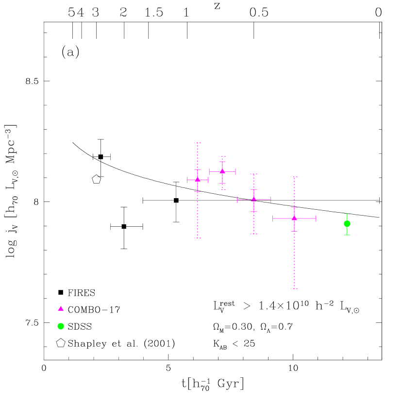
Figure 2.— The rest-frame optical luminosity density vs. cosmic age and redshift from galaxies with $K_{s,{\rm AB}}^{\rm tot}$ $<25$ and ${\rm L}_{\rm V}^{rest}$ $>$${\rm L}_{V}^{\rm thresh}$. For comparison we plot $j^{\rm rest}_{\lambda}$ determinations from other surveys down to our ${\rm L^{rest}_{\lambda}}$ limits. The squares are those from our data, the triangles are from the Combo-17 survey (Wolf et al., 2003), the circle is that at $z=0.1$ from the SDSS (B03), and the pentagon is that from Shapley et al. (2001). The dotted errorbars on the COMBO-17 data indicate the rms field-to-field variation derived from the three spatially distinct COMBO-17 fields. The solid line is a power law fit to the FIRES, COMBO-17, and SDSS data of the form $j^{\rm rest}_{\lambda}(z)=j^{\rm rest}_{\lambda}(0)*(1+z)^{\beta}$.

4.2. The Cosmic Color

Using our measures of $j^{\rm rest}_{\lambda}$ we estimated the cosmic rest-frame color of all the visible stars which lie in galaxies with ${\rm L}_{\rm V}^{rest}$ $>1.4\times 10^{10}$${\rm~{}h_{70}^{-2}~{}L_{\odot}}$. We derived the mean cosmic $(U~{}-~{}B)_{rest}$ and $(B~{}-~{}V)_{rest}$ by using the $j^{\rm rest}_{\lambda}$ estimates from the previous section with the appropriate magnitude zeropoints. The measured colors for the FIRES data, the COMBO-17 data, and the SDSS data are given in Table 1. Emission line corrected $(U~{}-~{}B)_{rest}$ colors may be calculated by applying Equation 1 to the values in the table. For the FIRES and COMBO-17 data, uncertainty estimates are derived from the same bootstrapping simulation used in § 4.1. In this case, however, the COMBO-17 and SDSS errorbars do not include an extra component from errors in the transformation to rest-frame luminosities, since these transformation errors may be correlated in a non-trivial way.

The bluing with increasing redshift which could have been inferred from Figure 2 is seen explicitly in Figure 3. The color change towards higher redshift occurs more smoothly than the evolution in $j^{\rm rest}_{\lambda}$, with our FIRES data meshing nicely with the COMBO-17 data. It is immediately apparent that the rms field-to-field errors for the COMBO-17 data are much less than the observed trend in color, in contrast to Figure 2. This explicitly shows that the integrated color is much less sensitive than $j^{\rm rest}_{\lambda}$ to field-to-field variations, even when such variations may dominate the error in the luminosity density. The COMBO-17 data at $z\lesssim 0.4$ are also redder than the local SDSS data, possibly owing to the very small central apertures used to measure colors in the COMBO-17 survey. The colors in the COMBO-17 data were measured with the package MPIAPHOT using using the peak surface brightness in images smoothed all to identical seeing ($1\farcs 5$). Such small apertures were chosen to measure very precise colors, not to obtain global color estimates. Because of color gradients, these small apertures can overestimate the global colors in nearby well resolved galaxies, while providing more accurate global color estimates for the more distant objects. Following the estimates of this bias provided by Bell et al. (2003b), we increased the color errorbars on the blue side to 0.1 for the $z<0.4$ COMBO-17 data. It is encouraging to see that the color evolution is roughly consistent with a rather simple model and that it is much smoother than the luminosity density evolution, which is more strongly affected by cosmic variance.

We interpreted the color evolution as being primarily driven by a decrease in the stellar age with increasing redshift. Applying the $(B~{}-~{}V)_{rest}$ dependent emission line corrections inferred from local samples (See §3.2.1), we see that the effect of the emission lines on the color is much less than the magnitude of the observed trend. We can also interpret this change in color as a change in mean cosmic ${\rm M}/{\rm L}^{*}$ with redshift. In this picture, which is true for a variety of monotonic SFHs and extinctions, the points at high redshift have lower ${\rm M}/{\rm L}^{*}$ than those at low redshift. At the same time, however, the evolution in $j^{\rm rest}_{\rm V}$ with redshift is quite weak. Taken together this would imply that the stellar mass density $\rho_{*}$ is also decreasing with increasing redshift. We will quantify this in §4.3.

To show how our mean cosmic $(U~{}-~{}B)_{rest}$ and $(B~{}-~{}V)_{rest}$ colors compare to those of morphologically normal nearby galaxies, we overplot them in Figure 4 on the locus of nearby galaxies from Larson & Tinsley (1978). The integrated colors, at all redshifts, lie very close to the local track, which Larson & Tinsley (1978) demonstrated is easily reproduceable with simple monotonically declining SFHs and which is preserved in the presence of modest amounts of reddening, which moves galaxies roughly parallel to the locus. In fact, correcting our data for emission lines moved them even closer to the local track. While we have suggested that ${\rm M}/{\rm L}^{*}$ decreases with decreasing color, if we wish to actually quantify the ${\rm M}/{\rm L}^{*}$ evolution from our data we must first attempt to find a set of models which can match our observed colors and which we will later use to convert between the color and ${\rm M}/{\rm L}^{*}_{V}$. We overplot in Figure 4 two model tracks corresponding to an exponential SFH with $\tau=6$ Gyr and with $E(B-V)=0$, 0.15, and 0.35 (assuming a Calzetti et al. (2000) reddening law). These tracks were calculated using the 2000 version of the Bruzual & Charlot (1993) models and have $Z=Z_{\odot}$ and a Salpeter (1955) IMF with a mass range of 0.1-120$M_{\odot}$. Other exponentially declining models and even a constant star forming track all yield similar colors to the $\tau=6$ Gyr track. The measured cosmic colors at $z<1.6$ are fairly well approximated either of the reddening models. At $z>1.6$, however, only the $E(B-V)=0.35$ track can reproduce the data. This high extinction is in contrast to the results of P01 and Shapley et al. (2001) who found a mean reddening for LBGs of $E(B-V)\sim 0.15$. SY98 and Thompson, Weymann, & Storrie-Lombardi (2001), however, measured extinctions on this order for galaxies in the HDF-N, although the mean extinction from Thompson, Weymann, & Storrie-Lombardi (2001) was lower at $z>2$. The amount of reddening in our sample is one of the largest uncertainty in deriving the ${\rm M}/{\rm L}^{*}$ values, nonetheless, our choice of a high extinction is the only allowable possibility given the integrated colors of our high redshift data.

Although this figure demonstrates that the measured colors can be matched, at some age, by this simple $E(B-V)=0.35$ model, we must nevertheless investigate whether the evolution of our model colors are also compatible with the evolution in the measured colors. This is shown by the track in Figure 3. We have tried different combinations of $\tau$, $E(B-V)$, and $z_{start}$, but have not been able to find a model which fits the data well at all redshifts. The parameterized SFR($z$) curve of Cole et al. (2001) also provided a poor fit to the data. Given the large range of possible parameters, our data may not be sufficient to well constrain the SFH.

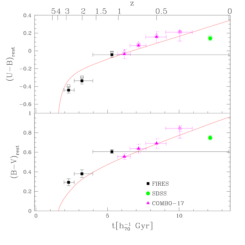
Figure 3.— The evolution of the cosmic color plotted against redshift and cosmic time for our data in addition to data from other $z\lesssim 1$ surveys. The squares are those from our data, the triangles are from the Combo-17 survey (Wolf et al., 2003), and the circle is that at $z=0.1$ from the SDSS (B03). The open symbols indicate the empirical emission line correction to the integrated colors derived using the spectroscopic and photometric data from the NFGS (Jansen et al., 2000b). The dotted errorbars on the COMBO-17 data indicate the field-to-field variation. Note that the integrated rest-frame color is much more stable than $j^{\rm rest}_{\lambda}$ against field-to-field variations. The COMBO-17 data point at $z=0.3$ has been given a color errorbar of 0.1 in the blueward direction and an open symbol to reflect the possible systematic biases resulting from their very small central apertures. We also overplot a model with an exponentially declining SFH with $\tau=6Gyr$, $E(B-V)=0.35$, and $z_{start}=4.0$ assuming a Calzetti et al. (2000) extinction law.

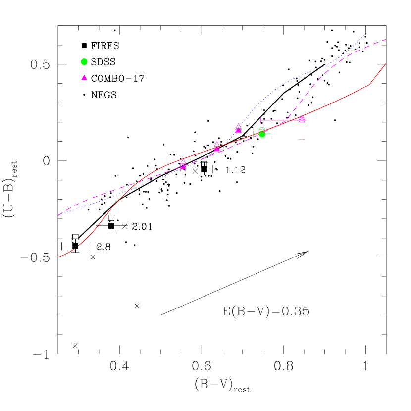
Figure 4.— The $(U~{}-~{}B)_{rest}$ vs. $(B~{}-~{}V)_{rest}$ at $z=$1.12, 2.01, and 2.8 of all the relatively unobscured stars in galaxies with ${\rm L}_{\rm V}^{rest}$ $>1.4\times 10^{10}$${\rm~{}h_{70}^{-2}~{}L_{\odot}}$. The thick solid black line is the local relation derived by Larson & Tinsley (1978) from nearby morphologically normal galaxies. The large symbols are identical to those in Figure 3. For clarity we do not plot the field-to-field errorbars for the COMBO-17 data. The small solid points are the colors of nearby galaxies from the NFGS (Jansen et al., 2000a), which have been corrected for emission lines. The small crosses are the NFGS galaxies which harbor AGN. The thin tracks correspond to an exponentially declining SFH with a timescale of 6 Gyr. The tracks were created using a Salpeter (1955) IMF and the 2000 version of the Bruzual & Charlot (1993) models. The dotted track has no extinction, the dashed track has been reddened by $E(B-V)=0.15$, and the thin solid track has been reddened by $E(B-V)=0.35$, using the Calzetti et al. (2000) extinction law. The black arrow indicates the reddening vector applied to the solid model track. The emission line corrected data lie very close the track defined by observations of local galaxies and the agreement with the models demonstrates that simple SFHs can be used to reproduce the integrated colors from massive galaxies at all redshifts.

4.3. Estimating ${\rm M}/{\rm L}^{*}_{V}$ and The Stellar Mass Density

In this subsection we describe the use of our mean cosmic color estimates to derive the mean cosmic ${\rm M}/{\rm L}^{*}_{V}$ and the evolution in $\rho_{*}$.

The main strength of considering the luminosity density and integrated colors of the galaxy population, as opposed to those of individual galaxies, lies in the simple and robust ways in which these global values can be modeled. When attempting to derive the SFHs and stellar masses of individual high-redshift galaxies, the state-of-the-art models for the broad-band colors only consider stellar populations with at most two separate components (SY98; P01; Shapley et al. 2001). Using their stellar population synthesis modeling, Shapley et al. (2001) proposes a model in which LBGs likely have smooth SFHs. On the other hand, SY98 concluded that they may only be seeing the most recent episode of star formation and that LBGs may indeed have bursting SFHs. This same idea was supported by P01 and Ferguson, Dickinson, & Papovich (2002) using much deeper NIR data. When using similar simple SFHs to model the cosmic average of the galaxy population, a more self-consistent approach is possible. While individual galaxies may, and probably do, have complex SFHs, the mean SFH of all galaxies is much smoother than that of individual ones.

Encouraged by the general agreement between the measured colors and the simple models, we attempted to use this model to constrain the stellar mass-to-light ratio ${\rm M}/{\rm L}^{*}_{V}$ in the rest-frame $V$-band, by taking advantage of the relation between color and log₁₀${\rm M}/{\rm L}^{*}$ found by Bell & de Jong (2001). For monotonic SFHs, the scatter of this relation remains small in the presence of modest variations in the reddening and metallicity because these effects run roughly parallel to the mean relation. Using the $\tau=6$ Gyr exponentially declining model, we plot in Figure 5 the relation between $(U~{}-~{}V)_{rest}$ and ${\rm M}/{\rm L}^{*}_{V}$ for the $E(B-V)=0$, 0.15, and 0.35 models. It is seen that dust extinction moves objects roughly parallel to the model tracks, reddening their colors, but making them dimmer as well and hence increasing ${\rm M}/{\rm L}^{*}_{V}$. Nonetheless, extinction uncertainties are a major contributor to our errors in the determination of ${\rm M}/{\rm L}^{*}_{V}$. We chose to derive ${\rm M}/{\rm L}^{*}_{V}$ from the $(U~{}-~{}V)_{rest}$ color instead of from the $(B~{}-~{}V)_{rest}$ color because at blue colors, where our high redshift points lie, $(B~{}-~{}V)_{rest}$ derived ${\rm M}/{\rm L}^{*}_{V}$ values are much more sensitive to the exact value of the extinction. This behavior likely stems from the fact that the $(U~{}-~{}V)_{rest}$ color spans the Balmer/4000${\rm\AA}$ break and hence is more age sensitive than $(B~{}-~{}V)_{rest}$. At the same time, while $(U~{}-~{}B)_{rest}$ colors are even less sensitive to extinction than $(U~{}-~{}V)_{rest}$, they are more susceptible to the effects of bursts.

We constructed our relation using a Salpeter (1955) IMF. The adoption of a different IMF would simply change the zeropoint of this curve, leaving the relative ${\rm M}/{\rm L}^{*}$ as a function of color, however, unchanged. As discussed in §4.2, this model does not fit the redshift evolution of the cosmic color very well. Nonetheless, the impact on our ${\rm M}/{\rm L}^{*}_{V}$ estimates should not be very large, since most smooth SFHs occupy very similar positions in the ${\rm M}/{\rm L}^{*}_{V}$ vs. $U-V$ plane.

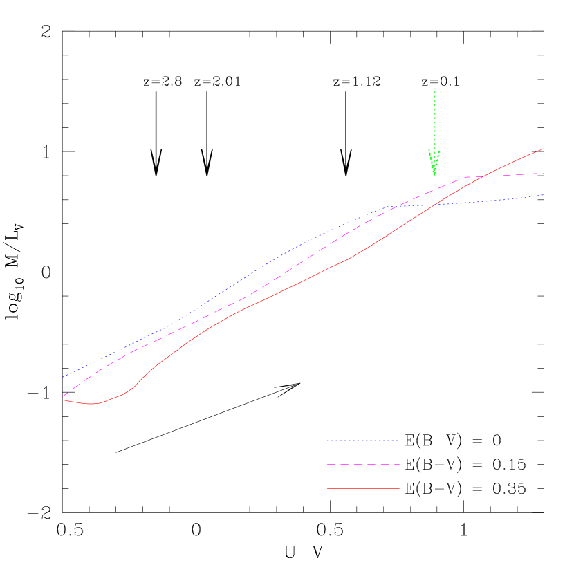
Figure 5.— The relation between $(U~{}-~{}V)$ and ${\rm M}/{\rm L}^{*}_{V}$ for a model track with an exponential timescale of 6 Gyr. The dotted line is for a model with $E(B-V)=0$, the dashed line for a model with $E(B-V)=0.15$, and the solid line is for a model reddened by $E(B-V)=0.35$ (using a Calzetti extinction law), which we adopt for our ${\rm M}/{\rm L}^{*}_{V}$ conversions. The vertical solid arrows indicate the colors of the three FIRES data points, the vertical dotted arrow indicates the color of the SDSS data, and the diagonal solid arrow indicates the vector used to redden the $E(B-V)=0$ model to $E(B-V)=0.35$. The labels above the vertical arrows correspond to the redshifts of the FIRES and SDSS data.

This relation breaks down in the presence of more complex SFHs. We demonstrate this in Figure 6 where we plot the $\tau=6$ Gyr track and a second track whose SFH is comprised of a 50 Myr burst at $t=0$, a gap of 2 Gyr, and a constant SFR rate for 1 Gyr thereafter, where 50% of the mass is formed in the burst. It is obvious from this figure that using a smooth model will cause errors in the ${\rm M}/{\rm L}^{*}_{V}$ estimate if the galaxy has a SFR which has an early peak in the SFH. At blue colors, such a early burst of SFR will cause an underestimate of ${\rm M}/{\rm L}^{*}_{V}$, a result similar to that of P01 and D03. At red colors, however, ${\rm M}/{\rm L}^{*}_{V}$ would be overestimated with the exact systematic offset as a function of color depending strongly on the detailed SFH, i.e. the fraction of mass formed in the burst, the length of the gap, and the final age of the stellar population.

The models show that the method may over- or underestimate the true stellar mass-to-light ratio if the galaxies have complex SFHs. It is important to quantify the errors on the global ${\rm M}/{\rm L}^{*}_{V}$ based on the mean $(U~{}-~{}V)_{rest}$ color and how these errors compare to those when determining the global ${\rm M}/{\rm L}^{*}_{V}$ value from individual ${\rm M}/{\rm L}^{*}_{V}$ estimates. To make this comparison we constructed a model whose SFH consist of a set of 10 Myr duration bursts separated by 90 Myr gaps. We drew galaxies at random from this model by randomly varying the phase and age of the burst sequence, where the maximum age was 4 Gyr. Next we estimated the total mass-to-light ratios of this sample by two different methods; first we determined the ${\rm M}/{\rm L}^{*}_{V}$ for the galaxies individually assuming the simple relation between color and mass-to-light ratio, and we took the luminosity weighted mean of the individual estimates to obtain the total ${\rm M}/{\rm L}^{*}_{V}$. This point is indicated by a large square in Figure 7 and overestimates the total ${\rm M}/{\rm L}^{*}_{V}$ by $\sim 70$%. Next we first add the light of all the galaxies in both $U$ and $V$, then use the simple relation between color and ${\rm M}/{\rm L}^{*}_{V}$ to convert the integrated $(U~{}-~{}V)_{rest}$ into a mass-to-light ratio. This method overestimates ${\rm M}/{\rm L}^{*}_{V}$ by much less, $\sim 35$%. This comparison shows clearly that it is best to estimate the mass using the integrated light. This is not unexpected; the star formation history of the universe as a whole is more regular than the star formation history of individual galaxies. If enough galaxies are averaged, the mean star formation history is naturally fairly smooth.

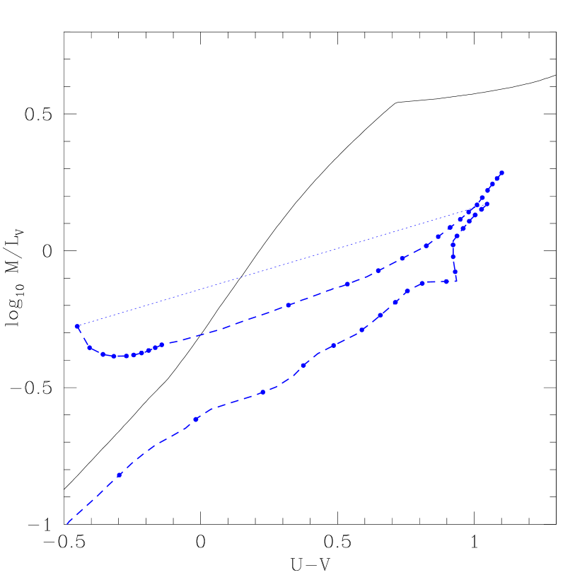
Figure 6.— The effect of an early burst of star formation on the relation between $(U~{}-~{}V)$ and ${\rm M}/{\rm L}^{*}_{V}$. The relation between $(U~{}-~{}V)$ and ${\rm M}/{\rm L}^{*}_{V}$ for a model track with an exponential timescale of 6 Gyr is show by the solid line. We also show a track for a SFH which includes a 50 Myr burst at $t=0$ followed by a gap of 2 Gyr and then a constant SFR rate for 1 Gyr thereafter, where the fraction of mass formed in the burst is 0.5. The track continues for a total time of 4.5 Gyr. The dots are placed at 100 Myr intervals and the dotted section of the line indicates the very rapid transition in color caused by the onset of the second period of star formation. Both tracks have the same extinction.

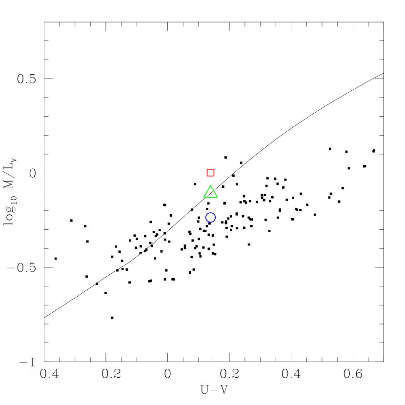
Figure 7.— A comparison of different measures of the global ${\rm M}/{\rm L}^{*}_{V}$ for a mock catalog of galaxies with bursting SFHs. The solid line represents the relation between $(U~{}-~{}V)$ and ${\rm M}/{\rm L}^{*}_{V}$ for a model track with an exponential timescale of 6 Gyr. The black dots show the true M/L’s of the model starbursting galaxies, as described in the text; the open circle shows the true luminosity weighted ${\rm M_{tot}}/{\rm L_{tot}}$ of the mock galaxies. The square shows the luminosity weighted ${\rm M}/{\rm L}^{*}_{V}$ derived by applying the simple model to the individual galaxies - in this case, the mean ${\rm M_{tot}}/{\rm L_{tot}}$ is overestimated by 70%. The triangle is the ${\rm M_{tot}}/{\rm L_{tot}}$ derived from the luminosity weighted mean color (or $(U-V)_{\rm tot}$) of the model galaxies. It overestimates ${\rm M_{tot}}/{\rm L_{tot}}$ by only 35%.

Using the relationship between color and ${\rm M}/{\rm L}^{*}_{V}$ we convert our $(U~{}-~{}V)_{rest}$ and $j^{\rm rest}_{\rm V}$ measurements to stellar mass density estimates $\rho_{*}$. The resulting $\rho_{*}$ values are plotted vs. cosmic time in Figure 8. We have included points for the SDSS survey created in an analogous way to those from this work, i.e. using the ${\rm M}/{\rm L}^{*}_{V}$ derived from the rest-frame color and multiplying it by $j_{V}^{\rm SDSS}$ for all galaxies with ${\rm L}_{\rm V}^{rest}$ $>$${\rm L}_{V}^{\rm thresh}$. The $\rho_{*}$ estimates are listed in Table 2. We have derived the statistical errorbars on the $\rho_{*}$ estimates by creating a Monte-Carlo simulation where we allowed $j^{\rm rest}_{\rm V}$ and $(U~{}-~{}V)_{rest}$ (and hence ${\rm M}/{\rm L}^{*}_{V}$) to vary within their errorbars. We then took the resulting distribution of $\rho_{*}$ values and determined the 68% confidence limits. As an estimate of our systematic uncertainties corresponding to the method we also determined ${\rm M}/{\rm L}^{*}_{V}$ from the $(U~{}-~{}B)_{rest}$ and $(B~{}-~{}V)_{rest}$ data using an identical relation as for the $(U~{}-~{}V)_{rest}$ to ${\rm M}/{\rm L}^{*}_{V}$ conversion. The $(U~{}-~{}B)_{rest}$ derived ${\rm M}/{\rm L}^{*}_{V}$ values were different from the $(U~{}-~{}V)_{rest}$ values by a factor of 1.02, 0.80, 0.95, and 1.12 for the $z=$0.1, 1.12, 2.01, and 2.8 redshift bins respectively. Likewise the $(B~{}-~{}V)_{rest}$ determined ${\rm M}/{\rm L}^{*}_{V}$ values changed by a factor of 0.99, 1.11, 1.15, and 0.80 with respect to the $(U~{}-~{}V)_{rest}$ values. While the $(U~{}-~{}V)_{rest}$ values are very similar to those derived from the other colors, the $(U~{}-~{}V)_{rest}$ color is less susceptible to dust uncertainties than the $(B~{}-~{}V)_{rest}$ data and less susceptible to the effects of bursts than the $(U~{}-~{}B)_{rest}$ data.

The derived mass density rises monotonically by a factor of $\sim 10$ all the way to $z\sim 0.1$, with our low redshift point meshing nicely with the local SDSS point.

Table 2${\rm M}/{\rm L}^{*}_{V}$ and Stellar Mass Density Estimates

$z$	log ${\rm M}/{\rm L}^{*}_{V}$	log $\rho_{*}$
	$[\frac{\mathrm{M_{\odot}}}{\mathrm{L_{\odot}}}]$	[$h_{70}~{}\mathrm{M_{\odot}}$Mpc-3]
$0.1\pm 0.1$	$0.54_{-0.03}^{+0.03}$	$8.49_{-0.05}^{+0.04}$
$1.12^{+0.48}_{-1.12}$	$0.13_{-0.06}^{+0.07}$	$8.14_{-0.10}^{+0.11}$
$2.01^{+0.40}_{-0.41}$	$-0.42_{-0.10}^{+0.09}$	$7.48_{-0.16}^{+0.12}$
$2.80^{+0.40}_{-0.39}$	$-0.70_{-0.12}^{+0.11}$	$7.49_{-0.14}^{+0.12}$

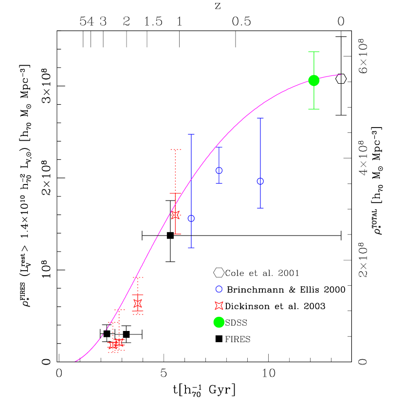
Figure 8.— The build-up of the stellar mass density as a function of redshift. The solid points are for galaxies with ${\rm L}_{\rm V}^{rest}$ $>1.4\times 10^{10}$${\rm~{}h_{70}^{-2}~{}L_{\odot}}$ and were derived by applying the $E(B-V)=0.35$ relation in Figure 5 to the $(U~{}-~{}V)_{rest}$ colors and $j^{\rm rest}_{\lambda}$ measurements from the FIRES (solid squares) and SDSS data (solid circle). The y-axis scale on the left side corresponds to the $\rho_{*}$ values for these points. The hollow points show the total stellar mass density measurements from the one-component models in the HDF-N (D03; hollow stars; calculated assuming solar metallicity), the CFRS (Brinchmann & Ellis 2000; hollow circles), and the 2dFGRS + 2MASS (Cole et al. 2001; hollow hexagon). The dotted errorbars on the D03 points reflect the systematic mass uncertainties resulting from metallicity and SFH changes. The y-axis scale on the right hand side corresponds to the $\rho_{*}$ estimates for these points. The relative scaling of the two axes was adjusted so that our SDSS $\rho_{*}$ estimate was at the same height as the total $\rho_{*}$ estimate of Cole et al. The solid curve is an integral of the SFR($z$) from Cole et al. (2001) which has been fit to extinction corrected data at $z\lesssim 4$.

5. Discussion

5.1. Comparison with other Work

Figure 8 shows a consistent picture of the build-up of stellar mass, both for the luminous galaxies and the total galaxy population. It is remarkable that the results from different authors appear to agree well given that the methods to derive the densities were different and that the fields are very small.

We compared our results to the total mass estimates of other authors in Figure 8. In doing this we must remember, because of our ${\rm L}_{\lambda}^{\rm thresh}$ cut, that we are missing significant amounts of light, and hence, mass. Assuming the SDSS luminosity function parameters, we lose 46% of the light at $z=0$. At $z=2.8$, however, we inferred a brightening of ${\rm L}_{*,V}$ by a factor of 1.7, implying that we go further down the luminosity function at high redshift, sampling a larger fraction of the total starlight. If we apply this brightening to the SDSS ${\rm L}_{*,V}$ we miss 30% of the light below our luminosity threshold at $z=2.8$. Hence, the fraction of the total starlight contained in our sample is rather stable as a function of redshift. To graphically compare our data to other authors we have scaled the two different axes in Figure 8 so that our derivation of the SDSS $\rho_{*}$ is at the same height of the total $\rho_{*}$ estimate of Cole et al. (2001). At $z<1$ we compared our mass estimates to those of Brinchmann & Ellis (2000). Following D03, we have corrected their published points to total masses by correcting them upwards by 20% to account for their mass incompleteness. The fraction of the total stars formed at $z<1$ agrees well between our data and that of SDSS and Brinchmann & Ellis. At $z>0.5$, we compared our results to those of D03. D03 calculated the total mass density, using the integrated luminosity density in the rest-frame B-band coupled with M/L measurements of individual galaxies. The fractions of the total stars formed in our sample (60%, 13%, and 9% at $z=$1.12, 2.01, and 2.8) are almost twice as high as those of D03. The results, however, are consistent within the errors.

We explored whether field-to-field variations may play a role in the discrepancy between the two datasets. D03 studied the HDF-N, which has far fewer ”red” galaxies than HDF-S (e.g., Labbé et al. 2003, Franx et al, 2003). If we omit the $J-K$ selected galaxies found by Franx et al. (2003) in the HDF-S, the formal ${\rm M}/{\rm L}^{*}_{V}$ decreases to 45% and 43% of the total values and the mass density decreases to 57% and 56% of the total values in the $z=2.01$ and $z=2.8$ bins respectively, bringing our data into better agreement with that from D03. This reinforces the earlier suggestion by Franx et al. (2003) that the $J-K$ selected galaxies contribute significantly to the stellar mass budget.

The errors in both determinations are dominated by systematic uncertainties, although our method should be less sensitive to bursts than that of D03 as it uses the light integrated integrated over the galaxy population.

We note that Fontana et al. (2003) have also measured the stellar mass density in the HDF-S using a catalog derived from data in common with our own. They find a similar, although slightly smaller evolution in the stellar mass density, consistent with our result to within the uncertainties.

5.2. Comparison with SFR($z$)

We can compare the derived stellar mass to the mass expected from determinations of the SFR as a function of redshift. We use the curve by Cole et al. (2001), who fitted the observed SFR as determined from various sources at $z\lesssim 4$. To obtain the curve in Figure 8 we integrated the SFR($z$) curve taking into account the time dependent stellar mass loss derived from the 2000 version of the Bruzual & Charlot (1993) population synthesis models.

We calculated a reduced $\chi^{2}$ of 4.3 when comparing all the data to the model. If, however, we omit the Brinchmann & Ellis (2000) data, the reduced $\chi^{2}$ decreases to 1.8, although the results at $z>2$ lie systematically below the curve. This suggests that some systematic errors may play a role, or that the curve is not quite correct. The following errors can influence our mass density determinations:

-Dusty, evolved populations: it is assumed that the dust is mixed in a simple way with the stars, leading to a Calzetti extinction curve. If the dust is distributed differently, e.g., by having a very extincted underlying evolved population, or by having a larger R value, the current assumptions lead to a systematic underestimate of the mass. If an underlying, extincted evolved population exists, it would naturally explain the fact that the ages of the Lyman-break galaxies are much younger than expected (e.g., P01, Ferguson et al. 2002). There may also be galaxies which contribute significantly to the mass density but are so heavily extincted that they are undetected, even with our very deep $K_{s}$-band data. If such objects are also actively forming stars, they may be detectable with deep submillimeter observations or with rest-frame NIR observations from SIRTF.

-Cosmic variance: the two fields which have been studied are very small. Although we use a consistent estimate of clustering from Daddi et al. (2003), red galaxies make up a large fraction of the mass density in our highest redshift bins. Since red galaxies have a very high measured clustering from $z\sim 1$ (e.g., Daddi et al. 2000, Mccarthy et al. 2001) up to possibly $z\sim 3$ (Daddi et al., 2003), large uncertainties remain.

-Evolving Initial Mass Function: the light which we see is mostly coming from the most massive stars present, whereas the stellar mass is dominated by low mass stars. Changes in the IMF would immediately lead to different mass estimates but if the IMF everywhere is identical (as we assume), then the relative masses should be robust. If the IMF evolves with redshift, however, systematic errors in the mass estimate will occur.

-A steep galaxy mass function at high redshift: if much of the UV light which is used to measure the SFR at high redshifts comes from small galaxies which would fall below our rest-frame luminosity threshold then we may be missing significant amounts of stellar mass. Even the mass estimates of D03, which were obtained by integrating the luminosity function, are very sensitive to the faint end extrapolation in their highest redshift bin.

5.3. The Build-up of the Stellar Mass

The primary goal of measuring the stellar mass density is to determine how rapidly the universe assembled its stars. At $z\sim 2-3$, our results indicate that the universe only contained $\sim 10\%$ of the current stellar mass, regardless of whether we refer only to galaxies at ${\rm L}_{\rm V}^{rest}$ $>1.4\times 10^{10}$${\rm~{}h_{70}^{-2}~{}L_{\odot}}$ or whether we use the total mass estimates of other authors. The galaxy population in the HDF-S was rich and diverse at $z>2$, but even so it was far from finished in its build-up of stellar mass. By $z\sim 1$, however, the total mass density had increased to roughly half its local value, indicating that the epoch of $1<z<2$ was an important period in the stellar mass build-up of the universe.

A successful model of galaxy formation must not only explain our global results, but also reconcile them with the observed properties of individual galaxies at all redshifts. For example, a population of galaxies at $z\sim 1-1.5$ has been discovered (the so called extremely red objects or EROs), roughly half of which can be fit with formation redshifts higher than 2.4 (Cimatti et al., 2002) and nearly passive stellar evolution thereafter. Our results, which show that the universe contained only $\sim 10\%$ as many stars at $z\sim 2-3$ as today would seem to indicate that any population of galaxies which formed most of its mass at $z\gtrsim 2$ can at most contribute $\sim 10\%$ of the present day stellar mass density. At $z\sim 1-1.5$, where the EROs reside, the universe had assembled roughly half of its current stars. Therefore, this would imply that the old EROs contribute about $\sim 20\%$ of the mass budget at their epoch. Likewise, it should be true that a large fraction of the stellar mass at low redshift should reside in objects with mass weighted stellar ages corresponding to a formation redshift of $1<z<2$. In support of this, Hogg et al. (2002) recently have shown that $\sim 40\%$ of the local luminosity density at $0.7\mu m$, and perhaps $\sim 50\%$ of the stellar mass comes from centrally concentrated, high surface brightness galaxies which have red colors. In agreement with the Hogg et al. (2002) results, Bell et al. (2003a) and Kauffmann et al. (2003) also found that $\sim 50-75\%$ of the local stellar mass density resides in early type galaxies. Hogg et al. (2002) suggest that their red galaxies would have been formed at $z\gtrsim 1$, fully consistent with our results for the rapid mass growth of the universe during this period.

6. Summary & Conclusions

In this paper we presented the globally averaged rest-frame optical properties of a $K_{s}$-band selected sample of galaxies with $z<3.2$ in the HDF-S. Using our very deep $0.3-2.2\mu m$, seven band photometry taken as part of the FIRE Survey we estimated accurate photometric redshifts and rest-frame luminosities for all galaxies with $K_{s,{\rm AB}}^{\rm tot}$ $<25$ and used these luminosity estimates to measure the rest-frame optical luminosity density $j^{\rm rest}_{\lambda}$, the globally averaged rest-frame optical color, and the stellar mass density for all galaxies at $z<3.2$ with ${\rm L}_{\rm V}^{rest}$ $>1.4\times 10^{10}$${\rm~{}h_{70}^{-2}~{}L_{\odot}}$. By selecting galaxies in the rest-frame $V$-band, we selected them in a way much less biased by star formation and dust than the traditional selection in the rest-frame UV and much closer to a selection by stellar mass.

We have shown that $j^{\rm rest}_{\lambda}$ in all three bands rises out to $z\sim 3$ by factors of $4.9\pm 1.0$, $2.9\pm 0.6$, and $1.9\pm 0.4$ in the $U$, $B$, and $V$-bands respectively. Modeling this increase in $j^{\rm rest}_{\lambda}$ as an increase in ${\rm L}_{*}$ of the local luminosity function, we derive that ${\rm L}_{*}$ must have brightened by a factor of 1.7 in the rest-frame $V$-band.

Using our $j^{\rm rest}_{\lambda}$ estimates we calculate the $(U~{}-~{}B)_{rest}$ and $(B~{}-~{}V)_{rest}$ colors of all the visible stars in galaxies with ${\rm L}_{\rm V}^{rest}$ $>1.4\times 10^{10}$${\rm~{}h_{70}^{-2}~{}L_{\odot}}$. Using the COMBO-17 data we have shown that the mean color is much less sensitive to density fluctuations and field-to-field variations than either $j^{\rm rest}_{\lambda}$ or $\rho_{*}$. Because of their stability, integrated color measurements are ideal for constraining galaxy evolution models. The luminosity weighted mean colors lie close to the locus of morphologically normal local galaxy colors defined by Larson & Tinsley (1978). The mean colors monotonically bluen with increasing redshift by 0.55 and 0.46 magnitudes in $(U~{}-~{}B)_{rest}$ and $(B~{}-~{}V)_{rest}$ respectively out to $z\sim 3$. We interpret this color change primarily as a change in the mean stellar age. The joint colors can be roughly matched by simple SFH models if modest amounts of reddening ($E(B-V)<0.35$) are applied. In detail, the redshift dependence of $(U~{}-~{}B)_{rest}$ and $(B~{}-~{}V)_{rest}$ cannot be matched exactly by the simple models, assuming a constant reddening and constant metallicity. However, we show that the models can still be used, even in the face of these small disagreements, to robustly predict the stellar mass-to-light ratios ${\rm M}/{\rm L}^{*}_{V}$ of the integrated cosmic stellar population implied by our mean rest-frame colors. Variations in the metallicity does not strongly affect this relation and it holds for a variety of smooth SFHs. Even the IMF only affects the normalization of this relation, not its slope, assuming that the IMF everywhere is the same. The reddening, which moves objects roughly along this relation is, however, a large source of uncertainty. Using these ${\rm M}/{\rm L}^{*}_{V}$ estimates coupled with our $j^{\rm rest}_{\lambda}$ measurements, we derive the stellar mass density $\rho_{*}$. These globally averaged estimates of the mass density are more reliable than those obtained from the mean of individual galaxies determined using smooth SFHs, primarily because the cosmic mean SFH is plausibly much better approximated as being smooth, whereas the SFHs of individual galaxies are almost definitely not.

The stellar mass density, $\rho_{*}$, increases monotonically with increasing cosmic time to come into good agreement with the other measured values at $z\lesssim 1$ with a factor of $\sim 10$ increase from $z\sim 3$ to the present day. Within the random uncertainties, our results agree well with those of Dickinson, Papovich, Ferguson, & Budavári (2003) in the HDF-N although our $\rho_{*}$ estimates are systematically higher than in the HDF-N. Taken together, the HDF-N and HDF-S paint a picture in which only $\sim 5-15\%$ of the present day stellar mass was formed by $z\sim 2$. By $z\sim 1$, however, the stellar mass density had increased to $\sim 50\%$ of its present value, implying that a large fraction of the stellar mass in the universe today was assembled at $1<z<2$. Our $\rho_{*}$ estimates slightly underpredict the stellar mass density derived from the integral of the SFR($z$) curve at $z>2$. A resolution of the small apparent discrepancy between different fields, and between the predictions from optical observations will in part require deeper NIR data, to probe further down the mass function, and wider fields with multiple pointings to control the effects of cosmic variance. In addition, large amounts of follow-up optical/NIR spectroscopy are required to help control systematic effects in the $z_{phot}$ estimates. The 25 square arcminute MS1054-03 data taken as part of FIRES and the ACS/ISAAC GOODS observations of the CDF-S region will be very helpful for such studies. Observations with SIRTF will also improve the situation by accessing the rest-frame NIR, where obscuration by dust becomes much less important. Finally, systematics in the ${\rm M}/{\rm L}^{*}$ estimates may exist because of a lack of constraint on the faint end slope of the stellar IMF.

We still have to reconcile global measurements of the galaxy population with what we know about the ages and SFHs of individual galaxies. Our globally determined quantities are quite stable and may serve as robust constraints on theoretical models, which must correctly model the global build-up of stellar mass in addition to matching the detailed properties of the galaxy population.

Appendix A Derivation of $z_{phot}$ Uncertainty

Given a set of formal flux errors, one way to broaden the redshift confidence interval without degrading the accuracy (as noticed in R01) is to lower the absolute $\chi^{2}$ of every $\chi^{2}$ $(z)$ curve without changing its shape (or the location of the minimum). By scaling up all the flux errors by a constant factor, we can retain the relative weights of the points in the $\chi^{2}$ without changing the best fit redshift and SED, but we do enlarge the redshift interval over which the templates can satisfactorily fit the flux points. Since we believe the disagreement between $z_{spec}$ and $z_{phot}$ is due to our finite and incomplete template set, this factor should reflect the degree of template mismatch in our sample, i.e., the degree by which our models fail to fit the flux points. To estimate this factor we first compute the fractional difference between the model and the data $\Delta_{i,j}$ for the j^th galaxy in the i^th filter,

$$\Delta_{i,j}=\frac{(f^{\rm mod}_{i,j}-f^{\rm dat}_{i,j})}{f^{\rm dat}_{i,j}}$$ (A1)

where $f^{\rm mod}$ are the predicted fluxes of the best-fit template combination and $f^{\rm dat}$ are our actual data. For each galaxy we calculated

$$\Delta_{j}=\sqrt{\frac{1}{N_{\rm filt}-1}\sum_{i=2}^{N_{\rm filt}}\Delta_{i,j}^{2}}$$ (A2)

where we have ignored the contributions of the $U$-band. While the $U$-band is important in finding breaks in the SEDs, the exact shapes of the templates are poorly constrained blueward of the rest-frame $U$-band and the $U$-data often deviates significantly from the best-fit model fluxes.

To determine the mean deviation of all of the flux points from the model $\Delta_{\rm dev}$ we then averaged over all galaxies in our complete FIRES sample with $K_{s,{\rm AB}}^{\rm tot}$ $<22$ (for which the systematic $z_{phot}$ errors should dominate over those resulting from photometric errors) to obtain

$$\Delta_{dev}=\frac{1}{N_{\rm gal}}\sum_{j=1}^{N_{\rm gal}}\left|\Delta_{j}\right|.$$ (A3)

We find $\Delta_{\rm dev}=0.08$, which includes both random and systematic deviations from the model. We modified the Monte-Carlo simulation of R01 by calculating, for each object j,

$$\left\langle{\rm\frac{S}{N}}\right\rangle_{j}=\sqrt{\frac{\sum_{i=2}^{N_{\rm filt}}\left(\frac{f_{i}}{\delta f_{i}}\right)^{2}}{N_{\rm filt}-1}}$$ (A4)

again excluding the $U$-band. We then scaled the flux errors, for each object, using the following criteria:

$$\delta f_{i}^{\prime}=\left\{\begin{array}[]{r@{\quad:\quad}l}\displaystyle\delta f_{i}&\displaystyle\left\langle{\rm\frac{S}{N}}\right\rangle_{j}\leq\frac{1}{\Delta_{\rm dev}}\\ \displaystyle\delta f_{i}\Delta_{\rm dev}\left\langle{\rm\frac{S}{N}}\right\rangle_{j}&\displaystyle\left\langle{\rm\frac{S}{N}}\right\rangle_{j}>\frac{1}{\Delta_{\rm dev}}\end{array}\right..$$ (A5)

The photometric redshift error probability distribution is computed using the $\delta f_{i}^{\prime}$’s. Note that this procedure will not modify the $z_{phot}$ errors of the objects with low $S/N$ where the $z_{phot}$ errors are dominated by the formal photometric errors. The resulting probability distribution is highly non-Gaussian and using it we calculate the upper and lower 68% confidence limits on the redshift $z_{phot}^{hi}$ and $z_{phot}^{low}$ respectively. As a single number which encodes the total range of acceptable $z_{phot}$’s, we define $\delta z_{phot}$ $\equiv 0.5*(z_{phot}^{hi}-z_{phot}^{low})$.

Figure 6 from L03 shows the comparison of $z_{phot}$ to $z_{spec}$. For these bright galaxies, it is remarkable that our new photometric redshift errorbars come so close to predicting the difference between $z_{phot}$ and the true value. Some galaxies have large $\delta z_{phot}$ values even when the local $\chi^{2}$ minimum is well defined because there is another $\chi^{2}$ minimum of comparable depth that is contained in the 68% redshift confidence limits. There are galaxies with $\delta z_{phot}$ $<0.05$. Some of these are bright low redshift galaxies with large rest-frame optical breaks, which presumably place a strong constraint on the allowed redshift. Many of these galaxies, however, are faint and the $\delta z_{phot}$ is unrealistically low. Even though these faint galaxies have $\left\langle{\rm\frac{S}{N}}\right\rangle_{j}\leq\frac{1}{\Delta_{\rm dev}}$, they still can have high $S/N$ in the $B_{450}$ or $V_{606}$ bandpasses and hence have steep $\chi^{2}$ curves and small inferred redshift uncertainties. In addition, many of these galaxies have $z_{phot}$ $>2$ and very blue continuum longward of ${\rm Ly\alpha}$. The imposed sharp discontinuity in the template SEDs at the onset of HI absorption causes a very narrow minimum in the $\chi^{2}$ $(z)$ curve, and hence a small $\delta z_{phot}$, but likely differs from the true shape of the discontinuity because we use the mean opacity values of Madau (1995), neglecting its variance among different lines of sight.

It is difficult to develop a scheme for measuring realistic photometric redshift uncertainties over all regimes. The $\delta z_{phot}$ estimate derives the $z_{phot}$ uncertainties individually for each object, but can underpredict the uncertainties in some cases. Compared to the technique of R01 however, a method based completely on the Monte-Carlo technique is preferable because it has a straightforwardly computed redshift probability function. This trait is desirable for estimating the errors in the rest-frame luminosities and colors and for this reason we will use $\delta z_{phot}$ as our uncertainty estimate in this paper.

Appendix B Rest-Frame Photometric System

To define the rest-frame $U$, $B$, and $V$ fluxes we use the filter transmission curves and zeropoints tabulated in Bessell (1990), specifically his $UX$, $B$, and $V$ filters. The Bessell zeropoints are given as magnitude offsets with respect to a source which has constant $f_{\nu}$ and $AB=0$. The $AB$ magnitude is defined as

$$AB_{\nu}=-2.5*{\rm log}_{10}\langle f_{\nu}\rangle-48.58$$ (B1)

where $\langle f_{\nu}\rangle$ is the flux $f_{\nu}(\nu)$ observed through a filter $T(\nu)$ and in units of $ergs~{}s^{-1}cm^{-2}Hz^{-1}$. Given the zeropoint offset $ZP_{\nu}$ for a given filter, the Vega magnitude $m_{\nu}$ is then

$$m_{\nu}=AB_{\nu}-ZP_{\nu}=-2.5*{\rm log}_{10}\langle f_{\nu}\rangle-48.58-ZP_{\nu}.$$ (B2)

All of our observed fluxes and rest-frame template fluxes are expressed in $f_{\lambda}$. To obtain rest-frame magnitudes in the Bessell (1990) system, we must calculate the conversion from $f_{\lambda}$ to $f_{\nu}$ for the redshifted rest-frame filter set. The flux density of an SED with $f_{\lambda}(\lambda)$ integrated through a given filter with transmission curve $T(\lambda)$ is

$$\langle f_{\lambda}\rangle=\frac{\int f_{\lambda}(\lambda^{\prime})T^{\prime}(\lambda^{\prime})d\lambda^{\prime}}{\int T^{\prime}(\lambda^{\prime})d\lambda^{\prime}}$$ (B3)

or

$$\langle f_{\nu}\rangle=\frac{\int f_{\nu}(\nu^{\prime})T^{\prime}(\nu^{\prime})d\nu^{\prime}}{\int T^{\prime}(\nu^{\prime})d\nu^{\prime}}.$$ (B4)

Since

$$\int f_{\lambda}(\lambda^{\prime})T^{\prime}(\lambda^{\prime})d\lambda^{\prime}=\int f_{\nu}(\nu^{\prime})T^{\prime}(\nu^{\prime})d\nu^{\prime}$$ (B5)

we can convert to $\langle f_{\nu}\rangle$ through

$$\langle f_{\nu}\rangle=\langle f_{\lambda}\rangle*\frac{\int T^{\prime}(\lambda^{\prime})d\lambda^{\prime}}{\int T^{\prime}(\nu^{\prime})d\nu^{\prime}}$$ (B6)

and use $\langle f_{\nu}\rangle$ to calculate the apparent rest-frame Vega magnitude through the redshifted filter via Eq. B2.

Appendix C Estimating Rest-Frame Luminosities

We derive for any given redshift, the relation between the apparent AB magnitude $m_{\lambda_{z}}$ of a galaxy through a redshifted rest-frame filter, its observed fluxes $\langle f_{\lambda_{i},obs}\rangle$ in the different filters $i$, and the colors of the spectral templates. At redshift z, the rest-frame filter with effective wavelength $\lambda_{rest}$ has been shifted to an observed wavelength

$$\lambda_{z}=\lambda_{rest}\times(1+z)$$ (C1)

and we define the adjacent observed bandpasses with effective wavelengths $\lambda_{l}$ and $\lambda_{h}$ which satisfy

$$\lambda_{l}<\lambda_{z}\leq\lambda_{h}.$$ (C2)

We now define

$$C_{obs}\equiv m_{obs,\lambda_{l}}-m_{obs,\lambda_{h}}$$ (C3)

where $m_{obs,\lambda_{l}}$ and $m_{obs,\lambda_{h}}$ are the AB magnitudes which correspond to the fluxes $\langle f_{\lambda_{l},obs}\rangle$ and $\langle f_{\lambda_{h},obs}\rangle$ respectively. We then shift each template in wavelength to the redshift z and compute,

$$C_{templ}\equiv m_{templ,\lambda_{l}}-m_{templ,\lambda_{h}},$$ (C4)

where $m_{templ,\lambda_{l}}$ and $m_{templ,\lambda_{h}}$ are the AB magnitudes through the $\lambda_{l}$ and $\lambda_{h}$ observed bandpasses (including the atmospheric and instrument throughputs). We sort the templates by their $C_{templ}$ values, $C_{templ,a}$, $C_{templ,b}$, etc., and find the two templates such that

$$C_{templ,a}\leq C_{obs}<C_{templ,b}.$$ (C5)

We then define for the $a^{\rm th}$ template

$$C_{\lambda_{l},z,a}\equiv m_{templ,\lambda_{l}}-m_{templ,\lambda_{z}}$$ (C6)

where $m_{templ,\lambda_{z}}$ is the apparent AB magnitude of the redshifted $a^{\rm th}$ template through the redshifted $\lambda_{rest}$ filter. We point out that because our computations always involve colors, they are not dependent on the actual template normalization (which cancels out in the difference). Taking our observed color $C_{obs}$ and the templates with adjacent “observed” colors $C_{templ,a}$ and $C_{templ,b}$, we can interpolate between $C_{\lambda_{l},z,a}$ and $C_{\lambda_{l},z,b}$

$$m_{obs,\lambda_{l}}-m_{\lambda_{z}}=C_{\lambda_{l},z,a}+(C_{obs}-C_{templ,a})\times\left(\frac{C_{\lambda_{l},z,b}-C_{\lambda_{l},z,a}}{C_{templ,b}-C_{templ,a}}\right)$$ (C7)

and solve for $m_{\lambda_{z}}$.

When $C_{obs}$ lies outside the range of the $C_{templ}$’s, we simply take the two nearest templates in observed $C_{templ}$ space and extrapolate Eq. C7 to compute $m_{\lambda_{z}}$.

Equation C7 has the feature that $m_{\lambda_{z}}\approx m_{obs,\lambda_{l}}$ when $\lambda_{z}=\lambda_{l}$ (and hence when $C_{\lambda_{l},z,a}$ and $C_{\lambda_{l},z,b}\approx 0$). While this method still assumes that the templates are reasonably good approximations to the true shape of the SEDs it has the advantage that it does not rely on exact agreement. Galaxies whose observed colors fall outside the range of the templates can also be easily flagged. A final advantage of this method is that the uncertainty in $m_{\lambda_{z}}$ can be readily calculated from the errors in the observed fluxes.

From $m_{\lambda_{z}}$, we compute the rest-frame luminosity by applying the K-correction and converting to luminosity units

$$\frac{\rm L^{rest}}{\rm L_{\odot}}=10^{\displaystyle-0.4(m_{\lambda_{z}}-{\rm M_{\odot,\lambda_{rest}}}-ZP_{\lambda_{rest}})}\times\left(\frac{\rm D_{L}}{10pc}\right)^{2}\times(1+z)^{-1}\times h^{-2}$$ (C8)

where ${\rm M_{\odot,\lambda_{rest}}}$ is the absolute magnitude of the sun in the $\lambda_{rest}$ filter (${\rm M_{\odot,U}=+5.66}$, ${\rm M_{\odot,B}=+5.47}$, and ${\rm M_{\odot,V}=+4.82}$ in Vega magnitudes; Cox 2000), $ZP_{\lambda_{rest}}$ is the zeropoint in that filter (as in Eq. B2 but expressed at $\lambda$ and not at $\nu$), and ${\rm D_{L}}$ is the distance modulus in parsecs. Following R01, we correct this luminosity by the ratio of the $K_{s}^{\rm tot}$ flux to the modified isophotal aperture flux (see L03). This adjustment factor, which accounts both for the larger size of the total aperture and the aperture correction, changes with apparent magnitude and it ranges from 1.23, at $20<$$K_{s,{\rm AB}}^{\rm tot}$ $\leq 24$, to 1.69, at $24<$$K_{s,{\rm AB}}^{\rm tot}$ $\leq 25$, and it has an RMS dispersions of 0.17 and 0.49 in the two magnitude bins respectively.

The uncertainty in the derived ${\rm L^{rest}_{\lambda}}$ has contributions both from the observational flux errors and from the redshift uncertainty, which causes $\lambda_{z}$ to move with respect to the observed filters. The first effect is estimated by propagating the observed flux errors through Eq. C7. As an example, object 531 at $z_{phot}$ =2.20 has $K_{s,{\rm AB}}^{\rm tot}$ $=24.91$ and signal-to-noise in the $K_{s}$-band of 8.99 and 5.43 in our modified isophotal and total apertures respectively. The resultant error in ${\rm L}_{\rm V}^{rest}$ purely from flux errors is then $26\%$. At $K_{s,{\rm AB}}^{\rm tot}$ $\approx 24$, the typical signal-to-noise in the $K_{s}$-band increases to $\approx 13$ and $\approx 6.3$ in our modified isophotal and total apertures respectively and the error ${\rm L^{rest}_{\lambda}}$ decreases accordingly.

To account for the redshift dependent error in the calculated luminosity, we use the Monte-Carlo simulation described first in R01 and updated in §A. For each Monte-Carlo iteration we calculate the rest-frame luminosities and determine the 68% confidence limits of the resulting distribution. The 68% confidence limits in ${\rm L^{rest}_{\lambda}}$ can be highly asymmetric, just as for $z_{phot}$. For objects with $K_{s,{\rm AB}}^{\rm tot}$ $\lesssim 25$ we find that the contributions to the total ${\rm L^{rest}_{\lambda}}$ error budget are dominated by the redshift errors rather than by the flux errors.

References

- Arnouts et al. (2002) Arnouts, S. et al. 2002, MNRAS, 329, 355
- Baldry et al. (2002) Baldry, I. K. et al. 2002, ApJ, 569, 582
- Barger, Cowie, & Richards (2000) Barger, A. J., Cowie, L. L., & Richards, E. A. 2000, AJ, 119, 2092
- Bell & de Jong (2001) Bell, E. F. & de Jong, R. S. 2001, ApJ, 550, 212
- Bell et al. (2003a) Bell, E. F., McIntosh, D. H., Katz, N., & Weinberg, M. D. 2003, ApJ, 585, L117
- Bell et al. (2003b) Bell, E. F., Wolf, C., Meisenheimer, K., Rix, H.-W., Borch, A., Dye, S., Kleinheinrich, K., McIntosh, D. H. 2003, submitted to ApJ, astro-ph/0303394
- Benítez et al. (1999) Benítez, N., Broadhurst, T., Bouwens, R., Silk, J., & Rosati, P. 1999, ApJ, 515, L65
- Bertin & Arnouts (1996) Bertin, E. & Arnouts, S. 1996, A&AS, 117, 393
- Bessell & Brett (1988) Bessell, M. S. & Brett, J. M. 1988, PASP, 100, 1134
- Bessell (1990) Bessell, M. S. 1990, PASP, 102, 1181
- Blanton et al. (2001) Blanton, M. R. et al. 2001, AJ, 121, 2358
- Blanton et al. (2003a) Blanton, M. R. et al. 2003a, ApJ, in press (astro-ph/0209479)
- Blanton et al. (2003b) Blanton, M. R. et al. 2003b, AJ, 125, 2348
- Blanton et al. (2003c) Blanton, M. R. et al. 2003c, ApJ, 592, 819
- Bolzonella, Pelló, & Maccagni (2002) Bolzonella, M., Pelló, R., & Maccagni, D. 2002, A&A, 395, 443
- Brinchmann & Ellis (2000) Brinchmann, J. & Ellis, R. S. 2000, ApJ, 536, L77
- Bruzual & Charlot (1993) Bruzual A., G. & Charlot, S. 1993, ApJ, 405, 538
- Calzetti et al. (2000) Calzetti, D., Armus, L., Bohlin, R. C., Kinney, A. L., Koornneef, J., & Storchi-Bergmann, T. 2000, ApJ, 533, 682
- Casertano et al. (2000) Casertano, S. et al. 2000, AJ, 120, 2747
- Charlot & Longhetti (2001) Charlot, S. & Longhetti, M. 2001, MNRAS, 323, 887
- Chen et al. (2003) Chen, H. et al. 2003, ApJ, 586, 745
- Cimatti et al. (2002) Cimatti, A. et al. 2002, A&A, 381, L68
- Cohen et al. (2000) Cohen, J. G., Hogg, D. W., Blandford, R., Cowie, L. L., Hu, E., Songaila, A., Shopbell, P., & Richberg, K. 2000, ApJ, 538, 29
- Cole et al. (2001) Cole, S. et al. 2001, MNRAS, 326, 255
- Coleman, Wu, & Weedman (1980) Coleman, G. D., Wu, C. -C., & Weedman, D. W. 1980, ApJS, 43, 393
- Colless et al. (2001) Colless, M. et al. 2001, MNRAS, 328, 1039
- Cowie, Songaila, & Barger (1999) Cowie, L. L., Songaila, A., & Barger, A. J. 1999, AJ, 118, 603
- Cox (2000) Cox, A. N. 2000, Allen’s astrophysical quantities, (4th ed. New York: AIP Press; Springer)
- Cristiani et al. (2000) Cristiani, S. et al. 2000, A&A, 359, 489
- Daddi et al. (2000) Daddi, E., Cimatti, A., Pozzetti, L., Hoekstra, H., Röttgering, H. J. A., Renzini, A., Zamorani, G., & Mannucci, F. 2000, A&A, 361, 535
- Daddi et al. (2003) Daddi, E. et al. 2003, ApJ, 588, 50
- Dickinson, Papovich, Ferguson, & Budavári (2003) Dickinson, M., Papovich, C., Ferguson, H. C., & Budavári, T. 2003, ApJ, 587, 25
- Eisenhardt & Dickinson (1992) Eisenhardt, P. & Dickinson, M. 1992, ApJ, 399, L47
- Erb et al. (2003) Erb, D. K., Shapley, A. E., Steidel, C. C., Pettini, M., Adelberger, K. L., Hunt, M. P., Moorwood, A. F. M., & Cuby, J. 2003, ApJ, 591, 101
- Ferguson, Dickinson, & Papovich (2002) Ferguson, H. C., Dickinson, M., & Papovich, C. 2002, ApJ, 569, L65
- Fernández-Soto, Lanzetta, & Yahil (1999) Fernández-Soto, A., Lanzetta, K. M., & Yahil, A. 1999, ApJ, 513, 34
- Folkes et al. (1999) Folkes, S. et al. 1999, MNRAS, 308, 459
- Förster Schreiber et al. (2003) Förster Schreiber, N. et al. in preparation
- Fontana et al. (2000) Fontana, A., D’Odorico, S., Poli, F., Giallongo, E., Arnouts, S., Cristiani, S., Moorwood, A., & Saracco, P. 2000, AJ, 120, 2206
- Fontana et al. (2003) Fontana, A. et al. 2003, ApJ, 594, L9
- Franx et al. (2003) Franx, M. et al. 2003, ApJ, 587, L79
- Frenk et al. (1985) Frenk, C. S., White, S. D. M., Efstathiou, G., & Davis, M. 1985, Nature, 317, 595
- Fried et al. (2001) Fried, J. W. et al. 2001, A&A, 367, 788
- Fukugita, Shimasaku, & Ichikawa (1995) Fukugita, M., Shimasaku, K., & Ichikawa, T. 1995, PASP, 107, 945
- Fukugita et al. (1996) Fukugita, M., Ichikawa, T., Gunn, J. E., Doi, M., Shimasaku, K., & Schneider, D. P. 1996, AJ, 111, 1748
- Giavalisco et al. (1998) Giavalisco, M., Steidel, C. C., Adelberger, K. L., Dickinson, M. E., Pettini, M., & Kellogg, M. 1998, ApJ, 503, 543
- Giavalisco & Dickinson (2001) Giavalisco, M. & Dickinson, M. 2001, ApJ, 550, 177
- Glazebrook (2003b) Glazebrook, K. et al. 2003, in preparation
- Glazebrook et al. (2003a) Glazebrook, K. et al. 2003, ApJ, 587, 55
- Hauschildt, Allard, & Baron (1999) Hauschildt, P. H., Allard, F., & Baron, E. 1999, ApJ, 512, 377
- Hogg et al. (2002) Hogg, D. W. et al. 2002, AJ, 124, 646
- Huchra (1977) Huchra, J. P. 1977, ApJ, 217, 928
- Jansen et al. (2000a) Jansen, R. A., Franx, M., Fabricant, D., & Caldwell, N. 2000, ApJS, 126, 271
- Jansen et al. (2000b) Jansen, R. A., Fabricant, D., Franx, M., & Caldwell, N. 2000, ApJS, 126, 331
- Kashikawa et al. (2003) Kashikawa, N. et al. 2003, AJ, 125, 53
- Kauffmann, White, & Guiderdoni (1993) Kauffmann, G., White, S. D. M., & Guiderdoni, B. 1993, MNRAS, 264, 201
- Kauffmann et al. (1999) Kauffmann, G., Colberg, J. M., Diaferio, A., & White, S. D. M. 1999, MNRAS, 303, 188
- Kauffmann et al. (2003) Kauffmann, G. et al. 2003, MNRAS, 341, 33
- Kinney et al. (1996) Kinney, A. L., Calzetti, D., Bohlin, R. C., McQuade, K., Storchi-Bergmann, T., & Schmitt, H. R. 1996, ApJ, 467, 38
- Labbé et al. (2003) Labbé, I. et al. 2003, AJ, 125, 1107
- Lanzetta et al. (2002) Lanzetta, K. M., Yahata, N., Pascarelle, S., Chen, H., & Fernández-Soto, A. 2002, ApJ, 570, 492
- Larson & Tinsley (1978) Larson, R. B. & Tinsley, B. M. 1978, ApJ, 219, 46
- Lilly et al. (1995) Lilly, S. J., Le Fevre, O., Crampton, D., Hammer, F., & Tresse, L. 1995, ApJ, 455, 50
- Lilly et al. (1996) Lilly, S. J., Le Fevre, O., Hammer, F., & Crampton, D. 1996, ApJ, 460, L1
- Madau (1995) Madau, P. 1995, ApJ, 441, 18
- Madau, Pozzetti, & Dickinson (1998) Madau, P., Pozzetti, L., & Dickinson, M. 1998, ApJ, 498, 106
- Madau et al. (1996) Madau, P., Ferguson, H. C., Dickinson, M. E., Giavalisco, M., Steidel, C. C., & Fruchter, A. 1996, MNRAS, 283, 1388
- McCarthy et al. (2001) McCarthy, P. J. et al. 2001, ApJ, 560, L131
- Moorwood (1997) Moorwood, A. F. 1997, Proc. SPIE, 2871, 1146
- Norberg et al. (2002) Norberg, P. et al. 2002, MNRAS, 336, 907
- Papovich, Dickinson, & Ferguson (2001) Papovich, C., Dickinson, M., Ferguson, H. C., 2001, ApJ, 559, 620
- Pei, Fall, & Hauser (1999) Pei, Y. C., Fall, S. M., & Hauser, M. G. 1999, ApJ, 522, 604
- Pettini et al. (2000) Pettini, M., Steidel, C. C., Adelberger, K. L., Dickinson, M., & Giavalisco, M. 2000, ApJ, 528, 96
- Pettini et al. (2001) Pettini, M., Shapley, A. E., Steidel, C. C., Cuby, J., Dickinson, M., Moorwood, A. F. M., Adelberger, K. L., & Giavalisco, M. 2001, ApJ, 554, 981
- Pettini et al. (2002) Pettini, M., Rix, S. A., Steidel, C. C., Adelberger, K. L., Hunt, M. P., & Shapley, A. E. 2002, ApJ, 569, 742
- Poli et al. (2001) Poli, F., Menci, N., Giallongo, E., Fontana, A., Cristiani, S., & D’Odorico, S. 2001, ApJ, 551, L45
- Poli et al. (2003) Poli, F. et al. 2003, ApJ, 593, L1
- Rigopoulou et al. (2000) Rigopoulou, D. et al. 2000, ApJ, 537, L85
- Rudnick et al. (2003) Rudnick, G. et al. 2003, in preparation
- Rudnick et al. (2001) Rudnick, G., Franx, M., Rix, H.-W., Moorwood, A., Kuijken, K., van Starkenburg, L., van der Werf, P., Röttgering, H., Labbé, I. 2001, AJ, 122, 2205
- Salpeter (1955) Salpeter, E. E. 1955, ApJ, 121, 161
- Sawicki, Lin, & Yee (1997) Sawicki, M. J., Lin, H., & Yee, H. K. C. 1997, AJ, 113, 1
- Scalo (1986) Scalo, J. M. 1986, Fundamentals of Cosmic Physics, 11, 1
- Schade et al. (1999) Schade, D. et al. 1999, ApJ, 525, 31
- Seaton (1979) Seaton, M. J. 1979, MNRAS, 187, 73P
- Shapley et al. (2001) Shapley, A. E., Steidel, C. C., Adelberger, K. L., Dickinson, M., Giavalisco, M., & Pettini, M. 2001, ApJ, 562, 95
- Skrutskie et al. (1997) Skrutskie, M. F. et al. 1997, ASSL Vol. 210: The Impact of Large Scale Near-IR Sky Surveys, 25
- Somerville, Primack, & Faber (2001) Somerville, R. S., Primack, J. R., & Faber, S. M. 2001, MNRAS, 320, 504
- Steidel et al. (1996) Steidel, C. C., Giavalisco, M., Pettini, M., Dickinson, M., & Adelberger, K. L. 1996, ApJ, 462, L17
- Steidel et al. (1999) Steidel, C. C., Adqelberger, K. L., Giavalisco, M., Dickinson, M., & Pettini, M. 1999, ApJ, 519, 1
- Stoughton et al. (2002) Stoughton, C. et al. 2002, AJ, 123, 485
- Strauss et al. (2002) Strauss, M. A. et al. 2002, AJ, 124, 1810
- Thompson, Weymann, & Storrie-Lombardi (2001) Thompson, R. I., Weymann, R. J., & Storrie-Lombardi, L. J. 2001, ApJ, 546, 694
- Thompson (2003) Thompson, R. I. 2003, ApJin press, astro-ph/0306594
- van De Ven, van Dokkum, & Franx (2003) van de Ven, G., van Dokkum, P. G., & Franx, M. 2003, submitted to MNRAS, astro-ph/0211566
- van Dokkumet al. (2001) van Dokkum, P. G., Franx, M., Kelson, D. D., & Illingworth, G. D. 2001, ApJ, 553, L39
- van Dokkum et al. (2003) van Dokkum, P. G. et al. 2003, ApJ, 587, L83
- Vanzella et al. (2002) Vanzella, E. et al. 2002, A&A, 396, 847
- Williams et al. (1996) Williams, R. E. et al. 1996, AJ, 112, 1335
- Wilson et al. (2002) Wilson, G., Cowie, L. L., Barger, A. J., & Burke, D. J. 2002, AJ, 124, 1258
- Wolf et al. (2003) Wolf, C., Meisenheimer, K., Rix, H.-W., Borch, A., Dye, S., & Kleinheinrich, M. 2003, A&A, 401, 73
- York et al. (2000) York, D. G. et al. 2000, AJ, 120, 1579
- Zepf (1997) Zepf, S. E. 1997, Nature, 390, 377