Integral-field spectrophotometry of the quadruple QSO HE 0435$-$1223: Evidence for microlensing

We present the first spatially resolved spectroscopic observations of the recently discovered quadruple QSO and gravitational lens HE 0435$-$1223. Using the Potsdam Multi-Aperture Spectrophotometer (PMAS), we show that all four QSO components have very similar but not identical spectra. In particular, the spectral slopes of components A, B, and D are indistinguishable, implying that extinction due to dust plays no major role in the lensing galaxy. While also the emission line profiles are identical within the error bars, as expected from lensing, the equivalent widths show significant differences between components. Most likely, microlensing is responsible for this phenomenon. This is also consistent with the fact that component D, which shows the highest relative continuum level, has brightened by 0.07 mag since Dec 2001. We find that the emission line flux ratios between the components are in better agreement with simple lens models than broad band or continuum measurements, but that the discrepancies between model and data are still unacceptably large. Finally, we present a detection of the lensing galaxy, although this is close to the limits of the data. Comparing with a model galaxy spectrum, we obtain a redshift estimate of $z_{\mathrm{lens}}=0.44\pm 0.02$.

1 Introduction

HE 0435$-$1223 was first discovered in the course of the Hamburg/ESO survey for bright QSOs (Wisotzki et al. 2000), and recently found to be a rather spectacular example of a quadruply imaged QSO (Wisotzki et al. 2002; hereafter Paper I). The quasar is at a redshift of $z=1.689$ and had a total magnitude $g=17.8$ at the epoch of discovery, with evidence for significant variability. The conspicuous geometry of four blue point sources of similar brightness arranged with nearly perfect symmetry around a red elliptical galaxy left no doubt about the nature of this object as being gravitationally lensed. However, Paper I featured only a blended spectrum of all components, and a formal verification based on individual spectroscopy of each component is still pending. In this paper we present the first set of spatially resolved spectra of this quadruple QSO, obtained by integral field spectrophotometry.

Figure 1: Top row: Example PMAS data of HE 0435$-$1223, for different wavebands. The first three images are quasi-monochromatic (3.3 Å bandwidth), the right-hand image is averaged over a wide passband. Each image measures $8^{\prime\prime}\times 8^{\prime\prime}$m and each spatial pixel is $0\aas@@fstack{\prime\prime}5\times 0\aas@@fstack{\prime\prime}5$. The orientation is standard (North is to the top, East is to the left). The four QSO components are clearly resolved. Notice the strong shift of image centroids as a function of wavelength (cf. Fig. 2), caused by differential atmospheric refraction. Middle row: Corresponding model images consisting of four superposed Gaussians (for details see text). Bottom row: Residuals after subtracting the four point sources.

2 Observations and data reduction

We targeted HE 0435$-$1223 during the first regular (i.e. non-comissioning) observing run of the Potsdam Multi-Aperture Spectrophotometer PMAS, mounted at the Calar-Alto 3.5 m telescope for several nights between 2–7 September, 2002. Details of this new instrument are given elsewhere (Roth et al. 2000); here we only summarise its capabilities. PMAS currently consists of a $16\times 16$ elements microlens array (an upgrade to $32\times 32$ elements is planned) coupled by optical fibres to a purpose-designed spectrograph. The image scale is $0\aas@@fstack{\prime\prime}5$ per spatial pixel (‘spaxel’), thus the total field of view is $8^{\prime\prime}\times 8^{\prime\prime}$. We used the V300 grating, giving a spectral resolution of $\sim 6$ Å FWHM and a spectral range of $\sim 3300$ Å, from 3950  to 7250 Å in our preferred setting. The data were recorded by a SITe $2048\times 4096$ pixels CCD detector, read out in $2\times 2$ binned mode. PMAS also features an independent on-axis imaging camera with a $3\aas@@fstack{\prime}4\times 3\aas@@fstack{\prime}4$ field of view and a $1024\times 1024$ pixels detector, mainly used for acquisition and guiding (termed the AG camera henceforth).

At the observing date in early September, HE 0435$-$1223 became visible only very shortly before morning twilight, and only at airmasses of around 2. We revisited the object repeatedly and could record useful data at the end of three different nights, with exposure times of altogether $3\times 1800$ s and $1\times 1200$ s. The external (DIMM) seeing was usually around or slightly below $1^{\prime\prime}$, which translated into an effective seeing in our PMAS data of between $1\aas@@fstack{\prime\prime}1$ and $1\aas@@fstack{\prime\prime}3$. Wavelength calibration and tracing of the 256 fibre spectra were facilitated through exposures using an internal calibration unit before or after each science spectrum.

Observations of the spectrophotometric standard star Hz 4 in the morning twilight provided the data needed for flux calibration. Since the AG camera was equipped with a Johnson $V$ filter, we could also exploit the acquisition exposures to check and improve the spectrophotometric calibration accuracy. Despite the high airmass of HE 0435$-$1223 during the observations, the flux level measurements of corresponding quasar spectra taken in different nights were remarkably consistent, with deviations of the order of 1 %. This indicates both photometric observing conditions and a stable system. Notice that since the PMAS microlens array reimages the exit pupil of the telescope, there are no geometrical losses due to incomplete filling of the focal plane (as with some other integral-field instruments). PMAS is thus certainly suitable for accurate spectrophotometry, and we shall use this capability below.

The data were reduced using our own IDL-based software package P3d (Becker 2002). The reduction consists of standard steps such as debiasing and flatfielding using twilight exposures, and dedicated routines such as tracing and extracting the spectra of individual fibres and reassembling the data in form of a three-dimensional data cube. Wavelength calibration and rebinning to a constant spectral increment is also part of the reduction procedure. The top row of Fig. 1 shows as examples some quasi-monochromatic and synthetic broad-band images, giving a good representation of the image quality, in particular S/N level and angular resolution. In fact, the S/N measured in our PMAS data is fully consistent with expectations from pure shot noise.

3 Deblending of the QSO components

3.1 Procedure

Starting with the data cubes produced on output by the P3d package, we developed a simple but powerful scheme to extract all four QSO spectra simultaneously. The following considerations guided our strategy:

• Because of the small field of view, the point-spread function was not known a-priori, but had to be determined within the QSO data. Non-simultaneous observations of PSF calibrator stars were not considered an option, because of the significant temporal PSF variability at the site.

• Due to differential atmospheric refraction, the source centroids vary with wavelength relative to the grid of $16\times 16$ spatial pixels. This effect is particularly grave for our high-airmass data, leading to a shift of more than four pixels (i.e. $>2^{\prime\prime}$) over the spectral range covered (see Figs. 1 and 2).

• Over the substantial spectral range covered, the width of the PSF can not assumed to be constant. This effect turned out to be less relevant than expected in our data, cf. Fig. 3, but significantly affected other data taken in the same campaign.

Our adopted algorithm is conceptually similar, albeit somewhat more complex, to procedures already used by us and others for the simultaneous extraction of double QSO spectra in long-slit data (e.g., Smette et al. 1995).

In essence, the routine performs a multi-component fit of $n$ two-dimensional Gaussians plus a spatially constant background value to the data in each quasi-monochromatic image, using a modified Levenberg-Marquard minimisation scheme (Press et al. 1992). In the case of HE 0435$-$1223, we adopted $n=4$ for the four QSO components. At the chosen spectral range, it was not strictly necessary to include also the lensing galaxy; as discussed in Sect. 7 below, we have marginally detected the galaxy, although on a level not much above the PSF mismatch residuals.

On output, the procedure provides the fitted parameters and their standard errors in a table. Each Gaussian is basically characterised by six parameters per spectral element: centroids in $x$ and $y$, FWHM along major and minor axis, position angle, and amplitude. By including some prior knowledge we can reduce the number of free parameters: First, the values of FWHM are assumed to be the same for all four point sources. The process is then iterated: In an initial pass, all parameters are fitted freely. In subsequent passes, the centroids, FWHM values and position angles are replaced by smoothly varying polynomial functions of $\lambda$, as exemplified by Figs. 2 and 3. Once fitted, these parameters are held fixed and do not participate in the fitting process, leaving only the 4 amplitudes to be fitted in the final pass. Model and residual data cubes are constructed along for inspection (see Fig. 1). The procedure turned out to be robust and efficient, simultaneously providing deblended spectra and a reasonable PSF, as demonstrated by the small residuals in the bottom row of Fig. 1.

After the final pass, the product of fitted amplitudes and (FWHM)² gave the extracted number of counts per spectral element for each QSO component. A similar extraction performed for the spectrophotometric standard star Hz 4 provided a formal flux calibration. We note that the efficiency of PMAS at 4000 Å is still 30 % of its peak value at 6000–7000 Å, which is remarkably high for an integral field spectrograph.

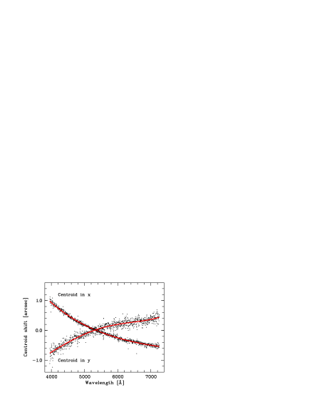
Figure 2: Centroid displacement as a function of wavelength, mainly due to differential atmospheric refraction. Each point corresponds to one quasi-monochromatic spectral layer. In the later fitting passes, the measured centroids are replaced by the polynomial approximation plotted by the solid lines.

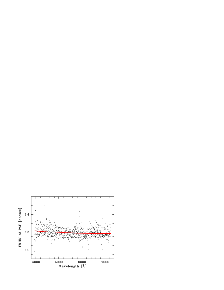
Figure 3: Same as Fig. 2, but for the full width at half maximum (average of major and minor axis) of the Gaussian PSF.

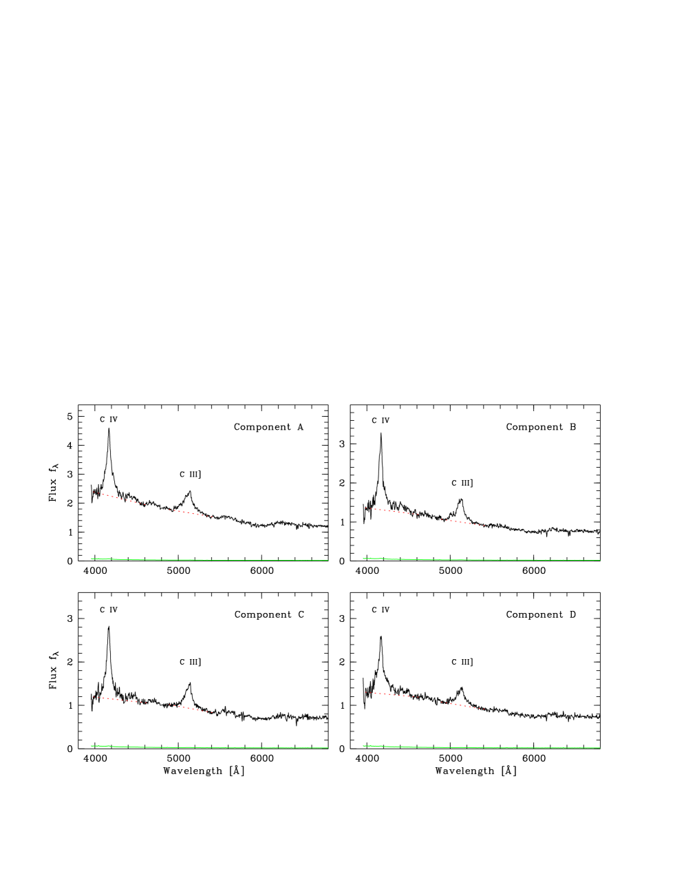
Figure 4: Extracted and coadded spectra of the four QSO components. The thin lines near zero represent the 1$\sigma$ error arrays. The adopted local continuum levels, used to derive emission line properties, are indicated by the dashed line segments.

3.2 Results

Visual inspection of the images confirms that the four components are well separated, with little or no significant mutual contamination (see Fig. 1). The extracted spectra from the four exposures of HE 0435$-$1223, obtained during three different nights, were combined using an inverse variance weighting scheme, which was also used to eliminate bad data values contaminated by cosmics or other spurious signals. Figure 4 shows the four final spectra together with the associated error vectors. The S/N in the continuum around $\lambda=5000$ Å is about 60 for component A and $\sim 40$ for the three fainter components B, C, and D.

Apparently, all four components show very similar and typical quasar spectra. While this is not really a surprise given the configuration of the system and the colours measured in Paper 1, it is nevertheless the first time that individual spectra of the components of HE 0435$-$1223 are published. The redshifts derived from the C iv and C iii] lines are identical to within the measurement accuracy: $z=1.6895\pm 0.0005$; the redshift scatter between the components is $\Delta z\simeq 0.0015$ (rms), corresponding to less than one spectral pixel.

4 Spectrophotometric Analysis

4.1 Broad-band fluxes

Our broad-band data from Paper 1 were taken with the Magellan telescope in SDSS filters $g$, $r$, and $i$ at two epochs, 14 Dec 2001 and 12 Feb 2002. In order to facilitate a straightforward comparison between these and our new PMAS data, we list synthetic broad-band magnitudes in Table 1, obtained by integrating over the $g$ and $r$ filter curves (our spectra do not cover the $i$ band). At the high S/N of our data, the formal errors of the synthesised broad-band values are far below 0.1 % and presumably outweighed by unknown systematics. The overall flux level in the $g$ band increased by 0.5 mag between Dec 2001 and Sep 2002. Already in Paper 1 we noted that HE 0435$-$1223 was variable, having brightened by almost 0.2 mag between Dec 2001 and Feb 2002. We did not detect variability on timescales of days: The fluxes measured in the three consecutive observing nights during this run are constant to within $\sim 1$ %.

The magnitude differences between the components are largely consistent with the values quoted in Paper 1, with one exception: Component D has brightened by 0.07 mag, from being the faintest component in the Magellan data to now at the same level as component B. We argue below that this is most likely due to microlensing.

We can also provide the first reliable colour measurements. The colours listed in Paper 1 were based on a very crude calibration scheme, tied to just one star with rather inaccurately known intrinsic colours. We find that the colours for all four components are basically identical, $(g-r)_{ABCD}=0.35$ with an rms scatter of 0.02 mag. In Paper 1 we found component C to be just slightly redder than the mean by 0.03 mag; although this is clearly at the edge of our measurement accuracy, we find that $(g-r)_{C}=0.38$, and the colour deviation is exactly reproduced in our new spectra. However, these results do not necessarily imply differences in continuum slope, as broad-band colours may well be influenced, at this accuracy level, by the different emission line equivalent widths discussed in the next section.

4.2 Emission lines

An important spectrophotometric diagnostic for gravitationally lensed QSOs is the comparison of emission line properties between components. While ideally the spectra of lensed quasar components should look identical, microlensing and other contaminating effects may lead to differences. In order to derive the emission line properties, we had to define the underlying continuum. Since we were not interested in a global continuum level, we defined two ad hoc continuum windows left and right of each line and connected these by straight lines (see Fig. 4). The windows were located at [3980 Å, 4020 Å] and [4530 Å, 4630 Å] for the C iv $\lambda$1550 line, and at [4890 Å, 4950 Å] and [5380 Å, 5440 Å] for the Al iii/C iii] $\lambda$1909 blend. The local continua thus derived are indicated by the dashed line segments in Fig. 4. This simple procedure worked quite well, although the continuum level at the blue side of the C iv line is poorly constrained due to the short wavelength cutoff of the spectra.

We then integrated the continuum-subtracted spectra within narrow windows centred on the emission line cores. The selection of these windows was to some extent arbitrary and mainly guided by the wish to avoid the low S/N wings which are most strongly affected by errors in the continuum estimate. The finally adopted integration windows were [4020 Å, 4300 Å] for C iv and [5075 Å, 5180 Å] for C iii]. Table 2 lists the results for all four components. We do not quote formal statistical errors because, as before, these are very small, typically $\sim 1$ % for the line fluxes, and almost certainly dominated by unknown systematical errors.

With high significance, the equivalent widths of the lines are not identical in the four components. This is already apparent from visual inspection of the spectra in Fig. 4. In other words: The flux ratios between the QSO components are different in the continuum and in the broad emission lines. We discuss this phenomenon in the next sections.

Finally, we also compared the emission line profiles. To this purpose we rescaled all continuum-subtracted lines to a common line integral and superimposed them pairwise. This is documented in Fig. 5, where the normalised C iv and C iii] lines of each of the components B, C, and D are plotted over A. As expected for a gravitationally lensed QSO, the individual line profiles are very similar and consistent with the assumption that they originate in the same object.

Table 1: Synthetic broad band magnitudes for HE 0435$-$1223, in the Johnson V and in the SDSS $g$ and $r$ bands (Vega magnitudes). Labelling of components as in Paper 1, i.e. clockwise.

Component	$V$	$g$	$r$	$g-r$
A	18.34	18.50	18.16	0.34
B	18.88	19.03	18.70	0.33
C	18.96	19.15	18.77	0.38
D	18.90	19.07	18.72	0.35
A+B+C+D	17.23	17.40	17.05	0.35

Table 2: Emission line fluxes and rest-frame equivalent widths for the four components. Fluxes are expressed in $10^{-16}\>\mathrm{erg}\>\mathrm{s}^{-1}\>\mathrm{cm}^{-1}$, equivalent widths in Å.

	C iv $\lambda$1550		C iii] $\lambda$1909
Component	$f$	$W_{0}$	$f$	$W_{0}$
A	120.1	19.2	60.3	13.5
B	90.4	24.2	46.3	17.2
C	86.0	26.8	42.3	16.9
D	66.2	18.3	31.7	11.8

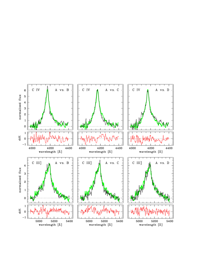
Figure 5: Pairwise comparison of normalised emission line profiles (upper row: C iv; lower row: C iii]). The light thick lines represent component A, the dark thin lines denote components B, C, and D, respectively. Below each panel we show also the difference between the profiles.

5 Spectral differences: Evidence for Microlensing

In the previous section we documented that despite the certain nature of HE 0435$-$1223 as a lensed QSO, the spectra of individual components are not strictly identical. Several effects can be invoked to explain spectral differences between lensed images: Foreground extinction, intrinsic variability, or microlensing. We discuss each of these in turn.

Extinction is probably not important in this object. The nearly identical (and typically quasar-like) colours of the four components imply that there is no significant differential extinction between these lines of sight. Although it is conceivable that all lines of sight suffer from the same amount of extinction, this would be an extreme coincidence if the dust column density were high. Furthermore, the lensing galaxy is a large elliptical (cf. Paper 1), not expected to contain large quantities of smoothly distributed dust in its outskirts. And of course the different equivalent widths of the emission lines cannot be explained by dust extinction at all, so there has to be at least one additional effect.

Intrinsic flux variability is certainly an issue in HE 0435$-$1223, as already discussed in Sect. 4.1. However, it is unlikely that variability is the explanation for the differences. From the lensing geometry, the light travel time delay between the images is predicted to be of the order of a few days (Paper 1). This means that very rapid and drastic intrinsic spectral changes would be needed in order to create differences between the images; we see no evidence at all for such violent variability. Even if there were such changes, escaping our attention, these would have to appear in each of the components consecutively within days. The fact that the spectra taken at three different nights look identical within the error bars (i.e. with an uncertainty of no more than a few per cent) speaks against significant short-time spectral variability.

Gravitational microlensing remains as the most straightforward explanation for the observed spectral differences between the four images. Within that scenario, microlensing affects the continuum and not the emission lines because of the sizes involved: The broad-line region in quasars is believed to be much larger than the typical cross-section of stellar mass lenses, and any magnification patterns are thus completely smeared out. On the other hand, the continuum-emitting region is orders of magnitude smaller than the BLR and certainly prone to microlensing (de)magnification, as most dramatically seen in the ‘Einstein Cross’ (e.g., Woźniak et al. 2000). Spectroscopy of that quasar (Lewis et al. 1998) showed also differences in the emission line equivalent widths very similar to the case discussed here. The most extreme known case of selective continuum amplification by microlensing is the ‘Double Hamburger’ HE 1104$-$1805 (Wisotzki et al. 1993), where there is even a strong chromatic effect, i.e. a wavelength-dependent amplification of the continuum (the spectrum gets bluer because the continuum region is smaller at shorter than at longer wavelengths and hence is more magnified; cf. Wambsganss & Paczynski 1991).

For all these objects as well as for HE 0435$-$1223, the emission line profiles are identical in all components. The spectral differences can then be interpreted as being entirely due to additional continuum contributions on top of the intrinsic ‘macrolensed’ spectra. Since microlensing is time-variable as a result of non-negligible effective transversal motions, this additional contribution is expected to vary. Interestingly, it is component D for which we find evidence for a relative brightening between Dec 2001 and Sep 2002; that component has the lowest equivalent widths and thus, in the microlensing picture, the highest continuum amplification. We conclude that microlensing is the only plausible explanation for the observed differences in line-to-continuum ratios. On the other hand, there is currently no indication of significant differential chromatic continuum amplification, since all components have so similar colours.

At this point it is useful to reconsider briefly the question whether the emission lines might also be affected by microlensing. The broad-line region in quasars (BLR) is generally held to be much bigger than the continuum region; for a quasar of the intrinsic (de-lensed) luminosity of HE 0435$-$1223, a BLR radius of the order of 100 light-days can be expected (Kaspi et al. (Kaspi et al. 2000)), two orders of magnitude larger than the Einstein radius of a solar-mass star at $z\simeq 0.4$. Any microlensing would therefore act on a small region of the BLR only, possibly causing some variations of the line profile as an observable signature, but certainly no significant overall amplification (cf. also Schneider & Wambsganss 1990). Even that effect cannot be strong in HE 0435$-$1223, since the line profiles are so similar (cf. Fig. 5). We therefore assume in the following that a clean distinction between the two domains exists: While the continuum source is very likely significantly amplified by microlensing, the emission lines remain more or less unaffected.

Table 3: Observed and predicted flux ratios between the four components: (1) C iv and C iii] emission lines; (2) continuum ratios at $\lambda=4580$ Å; (3) broad-band measurement from Paper 1; (4) flux ratios predicted from the model in Paper 1.

Ratio	lines	continuum	$g$ band	Model
B/A	0.77	0.62	0.60	1.11
C/A	0.71	0.54	0.57	1.04
D/A	0.56	0.61	0.55	0.68
C/B	0.93	0.87	0.95	0.94
D/B	0.73	0.98	0.93	0.61
D/C	0.79	1.12	0.97	0.65

6 Flux ratios

One interesting consequence of the microlensing interpretation is the expectation that the emission line fluxes should mirror the ‘true’ flux ratios of the four components, i.e. those given by macrolensing of the smooth galaxy potential alone. This is important for the construction of mass models for the lens: While flux ratios from broad-band photometry are notoriously unreliable because of the ever present possibility of microlensing, we suggest that emission line flux ratios can be directly used as additional model constraints. In Table 3 we provide the pairwise emission line flux ratios between the components. As a kind of ‘sanity check’, we also determined the corresponding continuum flux ratios, listed in the second column of Table 3. Since the spectral slopes are so similar, these values do not change significantly over the spectral range covered.

In Paper 1 it was found that a simple model involving a singular isothermal sphere plus external shear could reproduce the positions of the QSO components and of the lensing galaxy well within the error bars. However, the model (which was based on astrometric constraints only) predicted components B and C to be substantially brighter, by more than 0.5 mag relative to A and D, than observed in broad-band colours (cf. the last two columns in Table 3). Such disagreement between models and data has been seen in several other lensed QSOs as well, and two hypotheses have recently been proposed to account for these anomalies. On the one hand, they may indicate the presence of substructure in the lensing potential (e.g., Metcalf & Zhao 2002); or they could be due to microlensing at large optical depths, especially by suppressing the flux of saddle point images (Schechter & Wambsganss 2002). These two explanations differ significantly in their prediction of the flux ratios of extended source components. While the flux ratios should not depend strongly on source size in the case of a lens with substructure, a necessary consequence of the microlensing hypothesis is that the flux ratios should approach the ‘macrolens’ values as soon as the source is too extended to be affected by the microlens caustic network. This implies that if the size of the QSO broad-line region is already in this domain, emission-line flux ratios should be much closer to the model values if the model is realistic. There is at least one known quadruple QSO where this seems to be the case, namely B 1422$+$231 (cf. Impey et al. 1996).

This test can be performed with our spectrophotometric measurements of HE 0435$-$1223. Table 3 shows that the agreement between measured flux ratios and the model predictions is indeed much better if one uses the emission line values than with either broad band or continuum data. Components B and C are brighter in the emission lines than in the continuum, relative to A and D, while the ratios A/D and B/C do not change significantly. These changes are precisely in the direction approaching the model, just as predicted in the microlensing scenario by Schechter & Wambsganss.

However, the agreement is anything but good, and especially component A is still much brighter than is expected. As this could be due to shortcomings of the simple model which did not even take flux ratio constraints into account, we attempted to compute a new model. We used C. Keeton’s software tool lensmodel (Keeton 2001) to explore the consequences of adding measured flux ratios as additional constraints. For consistency, we stayed within the singular isothermal sphere plus external shear model (although we also tried some elliptical models). To our surprise, it was extremely difficult to make the predicted flux ratios approach the measured ones; the predictions tended to stay close to the Paper 1 values, which were based on the astrometry of the four QSO components alone (the position of the lensing galaxy was not considered to be sufficiently constrained, and therefore it was always left to float, as in Paper 1). This would only change when the flux ratio constraints were taken to be much tighter than the astrometric constraints. For example, we could roughly fit the flux ratios when allowing for several tenths of arc seconds of positional shifts, corresponding to a formal deviation of the order of more than $\sim 50\sigma$, which is totally unacceptable given the excellent astrometric quality of the Magellan data. Thus, even using the emission line measurements we failed to build a consistent model for the lensing potential that correctly reproduces both positions and flux ratios. But we recognise that a more sophisticated model of the lens mass distribution might well prove this statement premature. We have deliberately limited ourselves to explore only a narrow range of plausible configurations and now invite the experts in the field to follow up on us. Until then, we conclude that our measurements give some support to the microlensing hypothesis by Schechter & Wambsganss (2002), but that no wholly satisfying explanation for the flux ratios in HE 0435$-$1223 can yet be given.

Figure 6: Left panel: $4\times 4$ supersampled image of HE 0435$-$1223, coadded over a simulated 5500–7200 Å passband (see text for details). Right panel: Residual image after PSF subtraction, supersampled and coadded in the same way. Despite the significant PSF residuals, the lensing galaxy is clearly detected. The positions of the four QSO components and the lensing galaxy (from Paper 1) are marked by crosses.

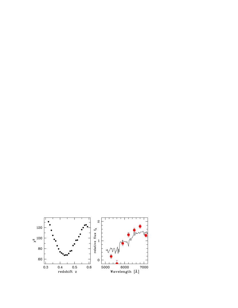
Figure 7: Redshift estimation for the lensing galaxy. Left panel: $\chi^{2}$ vs. redshift for model fit of 10 Gyr SSP to the binned residual spectrum at position of the lensing galaxy. Right panel: Residual spectrum with best-fit SSP model spectrum superimposed. For details see text.

7 The lensing galaxy

The Magellan $i$ band image presented in Paper I shows the lensing galaxy prominently, close to the geometric centre between the four QSO images. A similarly clean detection in our new PMAS data was not to be expected, for two reasons: (i) The much coarser pixel grid (0$\aas@@fstack{\prime\prime}$5 for PMAS vs. 0$\aas@@fstack{\prime\prime}$07 for Magellan+MagIC); (ii) the inferior effective seeing ($\ga 1\aas@@fstack{\prime\prime}1$ here vs. 0$\aas@@fstack{\prime\prime}$6 for Paper I). Furthermore, the nonavailability of a simultaneously obtained PSF reference made a clean PSF subtraction difficult. We have nevertheless attempted to detect the lensing galaxy, both in ‘imaging’ and in ‘spectroscopy’ mode. In our search we made use of some pieces of information available from Paper I. Firstly, we know the location of the galaxy relative to the QSO point sources. Secondly, we assume that its redshift is located within $0.3\la z\la 0.5$, to be in accordance with the photometric redshift estimate in Paper I. Notice that the narrowing of the range to $0.3\la z\la 0.4$ in Paper I using a luminosity-mass argument should be disregarded, as there was an error in computing the rest-frame absolute magnitude.

In order to partly overcome the coarse pixel grid limitation, we have exploited the fact that due to atmospheric refraction, the QSO centroid gradually shifts as a function of wavelength. In a way, this can be seen as almost equivalent to extensive dithering with respect to a broad-band image. The image is shifted by several pixels over the entire wavelength range, a fortuitous byproduct of the high airmass during observation. Within a band of just $\sim 1000$ Å, the displacement is already a good fraction of a pixel. Furthermore the number of samples taken is huge, roughly 300 for a 1000 Å bandpass. The information volume required for substantial subsampling therefore certainly exists. We have written a small application to coadd monochromatic data planes into a broad-band image, including a $4\times 4$ subsampling and applying the polynomial approximation to the centroid shifts described in Sect. 3.1.

Guided by the redshift prior on the lensing galaxy, we selected only the red part of the spectrum, $5500\,\mbox{\AA}<\lambda<7200\,\mbox{\AA}$. In addition, pieces of the spectrum heavily contaminated by night sky lines were left out. Both the original and the residual data cubes were run through this procedure. The result is shown in Fig. 6. The left panel shows that the four point sources are now much better defined than in the original coarse pixel data. In the right panel we find significant PSF residuals, featuring indications of positive central elevations and negative anullus-like patterns which document the limits of our simple assumption to model the PSF as a Gaussian. But we also find that the strongest residual is always positive and occurs very close to the expected position of the lensing galaxy. Relative to the position of component A, the difference from the value quoted in Paper 1 is only $\sim 0\aas@@fstack{\prime\prime}1$ in right ascension and $0\aas@@fstack{\prime\prime}2$ in declination. Going through the same exercise with a $\lambda<5500\,\mbox{\AA}$ image does not yield any discernible signal at that location. We therefore conclude that the detection is real and significant.

Thus encouraged, we looked whether spectral information, possibly even the lens redshift could be derived. We therefore extracted and coadded the spectra of a $2\times 2$ pixel block ($1^{\prime\prime}\times 1^{\prime\prime}$) at the expected location from each residual data cube. The result was an extremely noisy spectrum, with a signal that was on average positive above 6000 Å (S/N of $\sim 2$, for the original 3.3 Å wavelength steps) and zero or slightly negative below that. No QSO emission lines were present, indicating that cross-talk from the QSO point sources was negligible. Since it was hopeless to detect stellar absorption lines from the lensing galaxy in such low S/N data, we degraded the spectral resolution by summing the data into bins of 300 Å width, with the intention to use the overall spectral energy distribution for a redshift estimate. This is documented in Fig. 7. We assumed an old stellar population to dominate the SED of the lens (which has elliptical morphology, cf. Paper I), and cross-correlated the data with a solar metallicity, age of 10 Gyrs model galaxy spectrum from (Jimenez et al. 2000), kindly provided by R. Jimenez.

The left panel of Fig. 7 shows that $\chi^{2}(z)$ has a strong but flat-bottomed minimum between $z=0.43$ and $z=0.45$, and a turnover at $z=0.58$ towards another local minimum at much higher $z$. A lens redshift $z>0.5$ is not compatible with our prior assumptions; apart from its incompatibility with the colour measurement of Paper I, such a redshift would make the lens extremely massive. We therefore settle at a redshift estimate of $z_{\mathrm{lens}}=0.44\pm 0.02$, for which we show our best fit model overplotted over the binned residual spectrum. Note that we obtain consistent results (within the quoted error range) when analysing the individual exposures taken in different nights.

The model roughly reproduces the main feature of the data, its steep rising towards the red, but otherwise the fit is not good, and the error bars are probably underestimated. Selecting a younger stellar population would further degrade the fit quality, since already now our data are too red compared to the 10 Gyrs model (which is already the age of the universe at $z=0.44$). We conclude that our new lens redshift is a significant improvement over the rough colour estimate of Paper I, but the value is nevertheless tentative. A measurement of $z_{\mathrm{lens}}$ involving the detection of stellar absorption lines in the lensing galaxy is still indispensable.

8 Conclusions

We have presented the first spatially resolved spectra of the new quadruple QSO HE 0435$-$1223. The choice of an integral field spectrograph, and in particular the design of PMAS, enabled us to obtain high signal-to-noise data of spectrophotometric quality for all four quasar images simultaneously. The increasing availability of such instruments at many major telescopes opens a new window of opportunity to very efficiently observe gravitationally lensed QSOs – especially quadruple systems which are very hard to observe with traditional slit spectroscopy. Yet, two limitations need to be overcome to make integral field systems fully superior to other spectrographs, as far as gravitationally lensed quasars are concerned.

Firstly, resolving close systems requires an accurate knowledge of the point spread function. This is easily supplied by modern imaging cameras and multi-slit spectrographs, but the field of view of existing integral field units is generally much too small to simultaneously capture an isolated PSF reference star. One possible way out would be to use a second imaging device in parallel, such as is planned with the AG camera of PMAS. Another option might be to implement clever ‘PSF self-calibration’ algorithms, alleviating the need for an external PSF reference. Our simple approach involving just an analytic expression could be no more than a preparatory study to such techniques.

Secondly, there is usually a difficult trade-off between reaching a maximum field of view and the effective pixel size in the resulting images. Under excellent seeing conditions, a critical sampling of the PSF requires pixels no bigger than 0$\aas@@fstack{\prime\prime}$2, while most integral field spectrographs, including PMAS, have spaxels at least twice that size. As we have shown in this paper, image enhancement by supersampling to a finer pixel grid may be possible as a positive byproduct of differential atmospheric dispersion effects. But of course, the gain thus obtained will always be limited by the unavoidable convolution with the true pixel size.

With these provisions, a new quality level in the astrophysical study of microlensing in QSOs can be reached. Without major losses in observing time, simple broad band imaging can be replaced by a detailed spectrophotometric investigation. In this paper we have presented two pieces of evidence that microlensing is important in HE 0435$-$1223: spectral differences and variability. Future monitoring of microlensing-induced spectral variations in this object, and in similar targets, will constrain the structural properties of quasars on angular scales of sub-microarcseconds. Integral field spectroscopy is likely to become a tool of choice for this type of research.