Large Scale Cosmic Microwave Background Anisotropies and Dark Energy

Abstract

In this note we investigate the effects of perturbations in a dark energy component with a constant equation of state on large scale cosmic microwave background anisotropies. The inclusion of perturbations increases the large scale power. We investigate more speculative dark energy models with $w<-1$ and find the opposite behaviour. Overall the inclusion of perturbations in the dark energy component increases the degeneracies. We generalise the parameterization of the dark energy fluctuations to allow for an arbitrary constant sound speeds and show how constraints from cosmic microwave background experiments change if this is included. Combining cosmic microwave background with large scale structure, Hubble parameter and Supernovae observations we obtain $w=-1.02\pm 0.16$ (1$\sigma$) as a constraint on the equation of state, which is almost independent of the sound speed chosen. With the presented analysis we find no significant constraint on the constant speed of sound of the dark energy component.

1 Introduction

Observations of distant supernovae give strong indications that the expansion of the universe is accelerating (Perlmutter et al., 1997; Riess et al., 1998; Perlmutter et al., 1999; Riess et al., 2001). This is consistent with various other evidence, including recent precision observations of the cosmic microwave background (Spergel et al., 2003). These observations can in principle be explained by a cosmological constant term in Einstein’s equation of gravity. However, all that is really required to obtain accelerated expansion of the universe is the existence of a fluid component which dominates the universe today and which has a ratio of pressure to energy density of $w\equiv p_{\rm de}/\rho_{\rm de}<-1/3$. Quintessence models, which assume a scalar field as the dark energy component (Wetterich, 1988; Ratra & Peebles, 1988; Peebles & Ratra, 1988), differ from a cosmological constant model in that the equation of state parameter is not necessarily $w=-1$, and may be evolving. Furthermore a dark energy fluid with $w\neq-1$ will have perturbations.

In light of the recent cosmic microwave background (CMB) data of the Wilkinson Microwave Anisotropy Probe (WMAP) (Hinshaw et al., 2003) we re-investigate the constraints on a dark energy component with a constant equation of state and stress the importance of including perturbation in the dark energy. We note that perturbations have been included in the analysis of the WMAP team.

If the dark energy is not a cosmological constant, general relativity predicts that there will be perturbations. Even if dark energy is expected to be relatively smooth, for a consistent description of CMB perturbations it is necessary to include perturbations in the dark energy (Coble et al., 1997; Viana & Liddle, 1998; Caldwell et al., 1998; Ferreira & Joyce, 1998). We also allow for models with $w<-1$, as suggested by Caldwell (2002). These models might be realized in non-minimally coupled scalar field dark energy models (Amendola, 1999; Boisseau et al., 2000) or k-essence with non-canonical kinetic terms (Armendariz-Picon et al., 2000). Although the stability of such models is hard to achieve (Carroll et al., 2003), from an observational point of view one should not rule out the possibility in advance. Recent constraints from x-ray and type Ia Supernovae observation have constrained the equation of state to $w=-0.95\pm 0.30$ (Schuecker et al., 2003).

As mentioned above, most dark energy scenarios are motivated by canonical scalar field theories. This leads effectively to perturbations with a constant speed of sound of the fluctuations with ${\hat{c}}_{s}^{2}=1$. However k-essence models allow for an evolving sound speed (Armendariz-Picon et al., 2000; DeDeo et al., 2003). We therefore extend our analysis to models with constant $w$ and a constant speed of sound ${\hat{c}}_{s}^{2}$ as a free parameter.

2 Large scale cosmic microwave anisotropies

We will concentrate in this analysis on the behaviour of the temperature anisotropy power spectrum given by the covariance of the temperature fluctuation expanded in spherical harmonics

$$C_{l}=4\pi\int\frac{dk}{k}{\cal P}_{\chi}|\Delta_{l}(k,\eta_{0})|^{2}\,.$$ (1)

$\Delta_{l}(k,\eta_{0},\mu)$ gives the transfer function for each $\ell$, ${\cal P}_{\chi}$ is the initial power spectrum and $\eta_{0}$ is the conformal time today. On large scales the transfer functions are of the form

$$\Delta_{l}(k,\eta_{0})=\Delta_{l}^{\rm LSS}(k)+\Delta_{l}^{\rm ISW}(k)\,,$$ (2)

where $\Delta_{l}^{\rm LSS}(k)$ are the contributions from the last scattering surface given by the ordinary Sachs-Wolfe effect and the temperature anisotropy, and $\Delta_{l}^{\rm ISW}(k)$ is the contribution due to the change in the potential $\phi$ along the line of sight and is called the integrated Sachs-Wolfe (ISW) effect. The ISW contribution can be written (Sachs & Wolfe, 1967; Hu & Sugiyama, 1995)

$$\Delta_{l}^{\rm ISW}(k) = 2\int d\eta\,{\rm e}^{-\tau(\eta)}\phi^{\prime}j_{l}\left[k(\eta-\eta_{0})\right]$$

where $\tau(\eta)$ is the optical depth due to scattering of the photons along the line of sight, $j_{l}(x)$ are the spherical Bessel functions, and the dash denotes the derivative with respect to conformal time $\eta$. The frame-invariant potential $\phi$ can be defined in terms of the Weyl tensor, and is equivalent to the Newtonian potential in the absence of anisotropic stress (see Challinor & Lasenby (1999) for an overview of the covariant perturbation formalism we use here).

The Poisson equation relates the potential to the density perturbations via

$$k^{2}\phi=-4\pi Ga^{2}\overline{\delta\rho}\,,$$ (3)

where $\overline{\delta\rho}$ is the total comoving density perturbation. Thus the source term for the ISW contribution assuming only matter and dark energy is given by

$$k^{2}\phi^{\prime}=-4\pi G\frac{\partial}{\partial\eta}\left[a^{2}(\overline{\delta\rho}_{m}+\overline{\delta\rho}_{\rm de})\right]\;,$$ (4)

where the perturbations are evaluated in the rest frame of the total energy. The magnitude of the ISW contribution therefore depends on the late time evolution of the total density perturbation.

In general the fractional perturbations $\delta_{i}\equiv\delta\rho_{i}/\rho_{i}$ of a non-interacting fluid evolve as

$$\delta_{i}^{\prime}+3{\cal H}(c_{s,i}^{2}-w_{i})\delta_{i}+(1+w_{i})kv_{i}=-3(1+w_{i})h^{\prime}\,,$$ (5)

where ${\cal H}$ is the conformal Hubble parameter, $v_{i}$ is the velocity, $w_{i}\equiv p_{i}/\rho_{i}$, and $h^{\prime}=(\delta a/a)^{\prime}$, where the local scale factor $a$ is defined by integrating the Hubble expansion. The sound speed $c_{s}^{2}$ is frame-dependent, and defined as $c_{s}^{2}\equiv\delta p/\delta\rho$.

Neglecting anisotropic stress the potential $\phi$ evolves as

$$\phi^{\prime\prime}+3{\cal H}(1+\frac{p^{\prime}}{\rho^{\prime}})\phi^{\prime}+k^{2}\frac{p^{\prime}}{\rho^{\prime}}\phi+\left[(1+3\frac{p^{\prime}}{\rho^{\prime}}){\cal H}^{2}+2{\cal H}^{\prime}\right]\phi$$

$$=4\pi Ga^{2}(\delta p-\frac{p^{\prime}}{\rho^{\prime}}\delta\rho)\hfill,$$ (6)

where the RHS is a frame invariant combination. For a constant total equation of state parameter ${w_{\rm tot}}$ this becomes

$$\phi^{\prime\prime}+3{\cal H}(1+{w_{\rm tot}})\phi^{\prime}=4\pi Ga^{2}\overline{\delta p}.$$ (7)

In matter or cosmological constant domination the comoving pressure perturbation is zero on scales where the baryon pressure is negligible. In this case the growing mode is the solution $\phi=\rm{const}$, and there is no contribution to the ISW effect. However for varying ${w_{\rm tot}}$, as between matter and dark energy domination, or when there are dark energy perturbations, the potential will not be constant.

In general the evolution of the perturbations can be computed numerically. For a non-interacting fluid with constant $w_{i}$, defining the frame invariant quantity $\hat{c}_{s,i}^{2}$ (the fluid sound speed in the frame comoving with the fluid) we have the evolution equations

$$\delta_{i}^{\prime}+3{\cal H}(\hat{c}_{s,i}^{2}-w_{i})(\delta_{i}+3{\cal H}(1+w_{i})v_{i}/k)+\quad\quad$$

$$(1+w_{i})kv_{i}=-3(1+w_{i})h^{\prime}$$ (8)

$$v_{i}^{\prime}+{\cal H}(1-3\hat{c}_{s,i}^{2})v_{i}+kA=k\hat{c}_{s,i}^{2}\delta_{i}/(1+w_{i})\,,$$ (9)

where $A$ is the acceleration ($A=0$ in the $v_{m}=0$ frame (synchronous gauge), $A=-\Psi$ in the zero shear frame (Newtonian gauge)). We have assumed zero anisotropic stress, which is the case for matter and simple dark energy models. Also note that a varying equation of state factor will lead to extra contributions to the ISW effect (Corasaniti et al., 2003).

2.1 Scalar Field Dark Energy

In order to study the full evolution of the dark energy fluid including fluctuations we need to specify the speed of sound and hence its density and pressure perturbations. A simple way to achieve this, is by relating the dark energy to a scalar field. In order to be able to analyse models with an equation of state $w>-1$ as well as $w<-1$ we start with the Lagrangian (Carroll et al., 2003)

$${\cal L}_{\rm de}=\pm\frac{1}{2}(\partial_{\mu}\varphi)^{2}-V(\varphi)\;,$$ (10)

where the positive sign in front of the kinetic term corresponds to $w>-1$ solutions and the negative sign to $w<-1$,

$$\rho_{\rm de}=\pm\frac{1}{2}\dot{\varphi}^{2}+V\;,\quad\quad p_{\rm de}=\pm\frac{1}{2}\dot{\varphi}^{2}-V\,,$$ (11)

and dots denote normal time derivatives. The equations for the perturbations are therefore

$$\delta\rho_{\rm de} = \pm\dot{\varphi}\dot{(\delta\varphi)}+V_{,\varphi}\delta\varphi\pm A\dot{\varphi}{}^{2}$$ (12)

$$\delta p_{\rm de} = \pm\dot{\varphi}\dot{(\delta\varphi)}-V_{,\varphi}\delta\varphi\pm A\dot{\varphi}{}^{2}$$ (13)

where $A$ is the acceleration. In the frame in which the scalar field is unperturbed (the frame comoving with the dark energy, denoted by a hat), $\widehat{\delta\varphi}=0$ and so $\hat{c}_{s}^{2}\equiv\widehat{\delta p}/\widehat{\delta\rho}=1$.

If the equation of state $p_{\rm de}=w\rho_{\rm de}$ is constant, the dark energy density evolves like $\rho_{\rm de}=\rho_{{\rm de},0}\;a^{-3(1+w)}$. We can then identify this solution with a scalar field and its potential

$$V(\varphi) \equiv \frac{1-w}{2}\rho_{\rm de}\;,$$ (14)

$$\dot{\varphi}^{2} \equiv \pm(1+w)\rho_{\rm de}\;.$$ (15)

Clearly a constant equation of state makes a very unnatural quintessence model. However a large class of models are expected to be well described (at least as far as the CMB anisotropy is concerned) by an effective constant equation of state parameter. In this paper we do not explicitly consider dark energy models with an evolving equation of state.

In order to analyse the impact of the equation of state parameter of the dark energy component on the cosmic microwave background anisotropies we will first look into primary degeneracies originating from smaller scales in the temperature anisotropy power spectrum. As discussed in Melchiorri et al. (2002) the main impact is due to the change in the angular diameter distance toward the last scattering surface. The small scale CMB anisotropies in a flat universe are mainly sensitive to the physical cold dark matter and baryon densities and the angular diameter distance $d_{A}\propto\int[\Omega_{m}(1+z)^{3}+\Omega_{\rm de}(1+z)^{3(1+w)}]^{-1/2}$. Hence if $w$ is decreasing, we need to increase $\Omega_{\rm de}$ and for a flat universe decrease $\Omega_{\rm m}$ and therefore increase the Hubble parameter $H_{0}$ and therefore decrease $\Omega_{b}$ in order to obtain the same CMB anisotropy power spectrum.

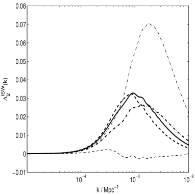
Figure 1: The quadrupole ($l=2$) contribution to the integrated Sachs-Wolfe effect. The solid line is for a $\Lambda$CDM universe, the dot dashed line for a universe with $w=-2$ and the dashed line for $w=-0.6$. For the other cosmological parameters see text. The bold lines are including perturbations in the dark energy component and the thin lines excluding them.

Let us assume that we can by some artificial mechanism suppress the fluctuations in the dark energy component. Note that in general this is not consistent with the equations of general relativity. Only in the case of a cosmological constant with $w=-1$ we recognise from Eqn. 5 that $\delta\rho_{\rm de}=0$ is a solution. We implement the equations in the frame comoving with the dark matter (synchronous gauge), and allow for a changing background equation of state but fix the dark energy perturbations to zero. We compare results from applying this (incorrect) recipe with those obtained using the full equations consistent with linear general relativity. In their rest frame the matter perturbations evolve like

$$\delta_{m}^{\prime\prime}+{\cal H}\delta_{m}^{\prime}=4\pi Ga^{2}\rho_{m}\overline{\delta_{m}}\,\quad\quad({\rm forced}\,\delta_{\rm de}=0),$$ (16)

which for matter domination ($w=0$) results in $\delta_{m}\propto a$. If we gradually decrease $w$ starting from $w=0$, the transition between matter and dark energy domination happens later and later, but more and more rapidly, and with a larger overall change in the equation of state. So we expect a smaller contribution to the ISW for values of $w$ closer to zero.

In Fig. 1 we show the quadrupole contribution $\Delta_{2}^{\rm ISW}(k)$ to the ISW. The solid line is for a $\Lambda$CDM universe with $w=-1$, $\Omega_{m}=0.3$, $\Omega_{b}=0.05$, $H_{0}=65~{}{\rm km}~{}{\rm s}^{-1}{\rm Mpc}^{-1}$, the thin dashed line is for $w=-0.6$, $\Omega_{m}=0.44$, $\Omega_{b}=0.073$, $H_{0}=54~{}{\rm km}~{}{\rm s}^{-1}{\rm Mpc}^{-1}$ and the thin dot-dashed for $w=-2$, $\Omega_{m}=0.17$, $\Omega_{b}=0.027$, $H_{0}=84~{}{\rm km}~{}{\rm s}^{-1}{\rm Mpc}^{-1}$. For all three models the spectral index is fixed to $n_{s}=1.0$ and the redshift of instantaneous complete reionization is $z_{\rm re}=17$. Without dark energy perturbations we clearly see that for $w=-0.6$ there is only a small contribution to the quadrupole from the ISW, while there is a large contribution for $w=-2$.

In the case of no dark energy perturbations for $w=-0.6$ there is a smaller ISW contribution than for a $\Lambda$CDM universe, and subsequently for $w=-2$ a larger ISW contribution.

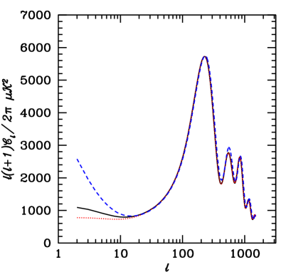
Figure 2: CMB angular power spectra for different dark energy models with no perturbations. The solid line is for a $\Lambda$CDM model, the dotted line for a model with $w=-0.6$ and dashed line $w=-2.0$. The parameters $\Omega_{c}$, $\Omega_{b}$ and $H_{0}$ are adjusted to show the degeneracies as mentioned in the text.

In Fig. 2 we show the entire temperature anisotropy power spectrum for the three degenerate models. We can see the increase in power on large scales by moving from the $w=-0.6$ over the $w=-1$ ($\Lambda$CDM) to the $w=-2$ model. If these were the true signatures of dark energy models on large scales we might be hopeful that by cross correlating large scale CMB anisotropies with x-ray or radio source power spectra (Boughn & Crittenden, 2003) one could break the angular diameter distance degeneracy of the small scale anisotropies.

The interplay between perturbations in the dark energy and the ISW is a subtle effect which we will discuss in the section 2.2. A simple way to understand the opposite behaviour of $w<-1$ models is that for $w<-1$ the density in the dark energy component is increasing with an expanding universe, while it is decreasing in a collapsing universe. Hence the dark energy perturbations are anti-correlated with the matter perturbations as they are sourced.

The bold lines in Fig. 1 correspond to the case which includes perturbations. Note that for $w=-1$, the perturbations are exactly zero. We see how the bold dot-dashed line ($w=-2$) is significantly lowered compared to the thin line, due to the contribution of the perturbation $\delta\rho_{\rm de}$, while for $w=-0.6$ (dashed line) the contribution is significantly enhanced.

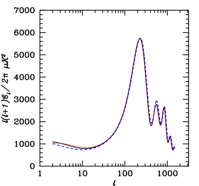
Figure 3: CMB angular power spectra for them dark energy models as in Fig. 2, but with dark energy perturbations.

In Fig. 3 we show the CMB temperature anisotropy spectrum for the three models this time including perturbations. We clearly see that the large differences obtained on large scales when we did not include perturbations in Fig. 2 have vanished. This is because for $w>-1$ the smaller overall change in the background equation of state is enhanced by the contribution due to the perturbations in the dark energy component. For $w<-1$ the large contribution from the different evolution of the background via the matter perturbations is partially cancelled by the contribution of the dark energy fluctuation. It seems difficult to obtain information about the nature of dark energy from large scale CMB information.

2.2 Generalised Dark Energy Perturbations

We turn now to the problem of how to describe dark energy perturbations without resolving to a scalar field. We should note as a reminder that we only resolved to a scalar field in order to have a prescription for calculating the perturbations, where we assumed the most simple kinetic term $\pm(\partial_{u}\varphi)^{2}$. These models have a speed of sound $\hat{c}_{s}^{2}=1$. However we have no idea what the dark energy actually is, so this assumption may be premature. For example, in a more generic class of dark energy models, so called k-essence, the kinetic term does not need to be of such a simple form (Armendariz-Picon et al., 2000) and the sound speed generally differs from one. In the most general case the speed of sound and the equation of state evolve with time, though clearly accounting for this is not feasible in general for parameter estimation. Here we generalise the dark energy parameterisation by introducing a constant sound speed ${\hat{c}}_{s}^{2}$ as a free parameter.

If ${\delta_{\rm de}}$ is initially zero, we see from Eqn. 8 that it is sourced by the other perturbations if $w\neq-1$ via the time evolution of the local scale factor, the source term $3(1+w)h^{\prime}$. An over density causes a decrease in the local expansion rate and so $h^{\prime}<0$. In this case a fluid starts to fall into overdensities if $w_{i}>-1$, but starts to fall out if $w_{i}<-1$. The subsequent evolution depends on the sound speed, as shown in Fig. 4. Consider the frame comoving with the dark matter (where $A=0$). When $k\ll{\cal H}$ the term $(1+w_{i})kv_{i}$ can be neglected, then the velocity and wavenumber only enter via the combination $(1+w_{i})v_{i}/k$. For large sound speeds the source term for the velocities is large and they are anti-damped, which leads to an almost $k$-independent evolution where the dark energy perturbations change sign at early times, and become the opposite sign to $\delta_{m}$. At late times when the dark energy becomes a significant fraction of the energy density, the total density perturbations are therefore smaller than without dark energy perturbations, there is a larger overal change in the potential, and the ISW contribution is increased. The sign reversal happens later for lower sound speeds as we see in Fig. 4 and for ${\hat{c}}_{s}^{2}\sim 1/3$ the perturbations never reverse. Thus the contribution to the ISW effect from the perturbations decreases with the sound speed. For $w<-1$ the effect is reversed, with the perturbations initially of opposite sign, and the contribution to the ISW effect increasing as the sound speed is decreased.

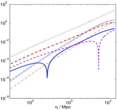
Figure 4: Evolution of $|\delta_{\rm de}|$ (thick) and $v_{\rm de}$ (thin) in the frame comoving with the dark matter perturbation (dotted line), for $w=-0.6$ and ${\hat{c}}_{s}^{2}=\{1,0.7,0.1\}$ (solid, dashed and dash-dotted lines), and $k=10^{-3}{\rm Mpc}^{-1}$. Note that we plot the absolute values of the fluctuations with amplitude normalized to unit initial curvature perturbation.

 

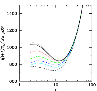
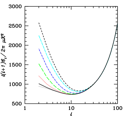
Figure 5: On the left the CMB anisotropies for the $w=-0.6$ model. The top solid line is with perturbations and the low dashed line for no perturbations. In between the speed of sound is decreasing from top to down with $c_{s}^{2}=0.2,0.05,0.01,0.0$. On the right the CMB anisotropies for the $w=-2.0$ model. The lower solid line is with perturbations and the top dashed line for no perturbations. In between the speed of sound is increasing from top to down with $c_{s}^{2}=0.0,0.01,0.05,0.2$. The thin dotted lines above (for $w=-0.6$) and below (for $w=-2$) correspond to sound speeds of $c_{s}^{2}=5.0$. Note that in both cases that $c_{s}^{2}=1.0$ corresponds to the solid line.

In Fig. 5 we show how the CMB temperature anisotropies change on large scales, for different constant ${\hat{c}}_{s}^{2}$. We see that if we decrease the sound speed gradually from ${\hat{c}}_{s}^{2}=1$ to ${\hat{c}}_{s}^{2}=0$ the ISW contribution becomes smaller as the dark energy clusters more with the matter, partly compensating the change in the potential due to the change in the background equation of state. Therefore cross - correlating the large scale CMB power spectrum with direct measures of the potential (Boughn & Crittenden, 2003) might be an excellent probe for the sound speed of the dark energy component, if the equation of state is different from $w=-1$.

3 Parameter constraints

In order to stress the importance of the inclusion of dark energy perturbations we will discuss their impact on the parameter estimation with CMB data. We included the perturbations into the camb code (Lewis et al., 2000) (based on cmbfast (Seljak & Zaldarriaga, 1996)) and performed a Markov-chain Monte Carlo parameter analysis using cosmomc (Lewis & Bridle, 2002). We varied six non-dark energy cosmological parameters with flat priors: the baryon density $\Omega_{b}h^{2}$, the cold dark matter density $\Omega_{\rm c}h^{2}$, the ratio of the sound horizon to the angular diameter distance at last scattering $\theta$, the damping of the small scale CMB power due to reionization $Z\equiv e^{-2\tau}$ (we assume $\tau<0.3$), the amplitude of the fluctuations $A_{s}$ and the spectral index of the primordial power spectrum $n_{s}$. In addition we varied the constant equation of state parameter of the dark energy component $w$, and where required the constant sound speed parameter in the range $-3<\log_{10}{\hat{c}}_{s}^{2}<2$. The Hubble parameter $H_{0}$ is derived from $\theta$ (Kosowsky et al., 2002), and the dark energy density from the requirement that the background universe is spatially flat. We assume negligible primordial tensor modes and neutrino mass, and include priors on the Hubble parameter from the Hubble Key project (Freedman et al., 2001), with $H_{0}=(72\pm 8)~{}{\rm km}~{}{\rm s}^{-1}{\rm Mpc}^{-1}$, and a weak prior $\Omega_{b}h^{2}=0.022\pm 0.002$ (1 $\sigma$) from Big Bang nucleosynthesis Burles et al. (2001). In addition to the CMB likelihood code provided by WMAP (Verde et al., 2003; Hinshaw et al., 2003; Kogut et al., 2003) (including the temperature-polarization cross-correlation data), we use CBI (Pearson et al., 2003) and ACBAR (Kuo et al., 2002) data for the smaller scales ($\ell>800$).

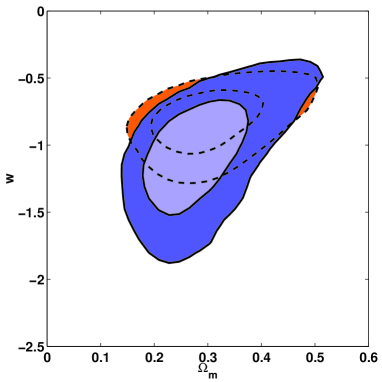
Figure 6: Marginalized 68% and 95% confidence contours from a combined analysis of the WMAP, ACBAR and CBI data together with a prior from BBN and HST, for an (incorrect) smooth dark energy component (dashed lines) and correctly including perturbations with ${\hat{c}}_{s}^{2}=1$ (solid lines).

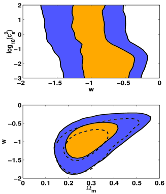
Figure 7: Marginalized 68% and 95% confidence contours from a combined analysis of the WMAP, ACBAR and CBI data together with a prior from BBN and HST, with ${\hat{c}}_{s}^{2}=1$ (dashed) and with ${\hat{c}}_{s}^{2}$ varying (solid).

In Fig. 6 we show the posterior confidence contours in the $\Omega_{m}-w$ plane. The dashed contours are from an analysis assuming no perturbations in the dark energy component, while the solid contours are with perturbations. We clearly see the different shape of the likelihood contours and how they open up to more negative values in $w$ if we include perturbations. This is a direct result of the difference between Figs. 2 and 3. Because the large ISW for $w<-1$ is not present if we include perturbations this part of the parameter space can not be excluded with CMB data. Furthermore the inclusion of perturbations leads to more stringent upper bounds on the equation of state $w$. This is because as we increase the large scale CMB power due to the perturbations (for $w>-1$), the relatively low quadrupole and octopole disfavour these models. In Fig. 7 we show the constraints from additionally varying a constant sound speed. This slightly favours values of $w>-1$, where low sound speeds lead to a smaller ISW contribution at the lowest $\ell$. For $w<-1$ the contours broaden to include large sound speeds which also give somewhat smaller low multipoles.

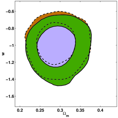
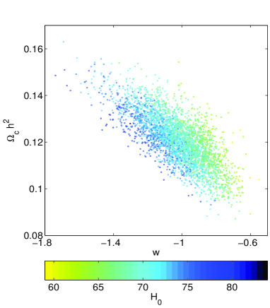
Figure 8: Top: 68% and 95% contours for a combined analysis of the CMB data, 2dF, SNe, HST and BBN with ${\hat{c}}_{s}^{2}=1$ (solid) and marginalizing over ${\hat{c}}_{s}^{2}$ (dashed). Bottom: Samples from the posterior distribution for ${\hat{c}}_{s}^{2}=1$ with the same data as above.

Finally we performed an analysis where we also included the data from the Supernovae Cosmology Project (SCP) (Perlmutter et al., 1999) and the two degree field (2dF) galaxy redshift survey (Percival et al., 2001). The information from the 2dF large scale structure combined with the prior from the Hubble Key Project constrains the matter contents, while the Supernovae (SNe) information is complementary. In Fig. 8 we show the result of this combined analysis, with and without marginalizing over a varying sound speed ${\hat{c}}_{s}^{2}$. The mean value for scalar field models with ${\hat{c}}_{s}^{2}=1$ is $w=-1.02$, strikingly close to a cosmological constant, however the 95% marginalized confidence limit $-1.37<w<-0.74$ still allows a lot of room for different dark energy scenarios. Allowing for a different value of the sound speed only slightly shifts the constraints on $w$ to higher values, with the 95% result $-1.32<w<-0.70$. The dominant remaining degeneracies are illustrated in the scatter plot in Fig. 8, where we see how the constraints depend on the preferred value of the Hubble parameter $H_{0}$.

4 Conclusions

In this note we have re-analysed the constraints on the equation of state parameter $w$ of dark energy mainly from CMB observations. We have emphasised the fact that it is essential to include perturbations in the dark energy component to perform the analysis. The large scale anisotropies look very different when perturbations are included and it seems hard to use large scale CMB information to break the degeneracies.

Furthermore we studied models with an equation of state with $w<-1$. Our findings are similar to the recently extended version of the WMAP analysis (Spergel et al., 2003; Verde et al., 2003). Clearly models with $w<-1$ are under a lot of pressure for theoretical reasons, since they violate the weak energy condition and might be unstable. However an effective description of dark energy with non-canonical kinetic terms and a momentum cut-off might be a valid model for such a scenario (Armendariz-Picon et al., 2000; Carroll et al., 2003).

Finally we found as a posterior mean value for the equation of state parameter $w=-1.02$, though this conclusion might depend somewhat on our choice of a constant equation of state parameterisation (Maor et al., 2002). Furthermore we do not find significant constraints on the value of a constant speed of sound. We note that in a recent paper Bean & Doré (2003) find a $1-\sigma$ detection for a low sound speed. This is probably due to the fact that they keep parameters like the the physical matter density fixed. However cross-correlating the large scale CMB data with large scale structure measurements could improve these constraints (Boughn & Crittenden, 2003; Bean & Doré, 2003).

To conclude a cosmological constant is certainly very consistent with the current data, however the 95% limits on the effective equation of state do not rule out most scalar field dark energy models. Hence we need better observations to constrain dark energy models and to be able to distinguish them from a cosmological constant. While large scale CMB observations are limited by cosmic variance, the proposed Supernovae Acceleration Probe - SNAP could fulfil this objective (Weller & Albrecht, 2002).

References

- Amendola (1999) Amendola L., 1999, Phys. Rev., D60, 043501
- Armendariz-Picon et al. (2000) Armendariz-Picon C., Mukhanov V., Steinhardt P. J., 2000, Phys. Rev. Lett., 85, 4438
- Bean & Doré (2003) Bean R., Doré O., 2003, astro-ph/0307100
- Boisseau et al. (2000) Boisseau, B., Esposito-Farèse, G., Polarski, D., Starobinsky, A. A., 2000, Phys. Rev. Lett., 85, 2236
- Boughn & Crittenden (2003) Boughn S., Crittenden R., 2003, astro-ph/0305001
- Burles et al. (2001) Burles S., Nollett K. M., Turner M. S., 2001, Astrophys. J., 552, L1
- Caldwell et al. (1998) Caldwell R., Dave R., Steinhardt P., 1998, Phys. Rev. Lett., 80, 1582
- Carroll et al. (2003) Carroll S. M., Hoffman M., Trodden M., 2003, astro-ph/0301273
- Challinor & Lasenby (1999) Challinor A., Lasenby A., 1999, Astrophys. J., 513, 1
- Coble et al. (1997) Coble K., Dodelson S., Friedman J., 1997, Phys. Rev. D, D 55, 1851
- Corasaniti et al. (2003) Corasaniti, P. S., Bassett, B., Ungarelli, C., Copeland, E. J,, 2003, Phys. Rev. Lett., 90, 091303
- DeDeo et al. (2003) DeDeo S., Caldwell R. R., Steinhardt P. J., 2003, Phys. Rev., D67, 103509
- Ferreira & Joyce (1998) Ferreira P., Joyce M., 1998, Phys. Rev. D, D 58, 023503
- Freedman et al. (2001) Freedman W., et al., 2001, Ap. J., 553, 47
- Hinshaw et al. (2003) Hinshaw G., et al., 2003, Ap. J. S., 148, 135
- Hu & Sugiyama (1995) Hu W., Sugiyama N., 1995, Astrophys. J., 444, 489
- Kogut et al. (2003) Kogut A., et al., 2003, Ap. J. S., 148, 161
- Kosowsky et al. (2002) Kosowsky A., Milosavljevic M., Jimenez R., 2002, Pys. Rev. D, 66, 063007
- Kuo et al. (2002) Kuo C. L., et al., 2002, astro-ph/0212289
- Lewis & Bridle (2002) Lewis A., Bridle S., 2002, Phys. Rev., D66, 103511
- Lewis et al. (2000) Lewis A., Challinor A., Lasenby A., 2000, Astrophys. J., 538, 473
- Maor et al. (2002) Maor I., Brustein R., McMahon J., Steinhardt P. J., 2002, Phys. Rev., D65, 123003
- Melchiorri et al. (2002) Melchiorri A., Mersini L., Odman C. J., Trodden M., 2002, astro-ph/0211522
- Pearson et al. (2003) Pearson T. J., et al., 2003, Ap. J., 591, 556
- Peebles & Ratra (1988) Peebles P., Ratra B., 1988, Ap. J., 325, L17
- Percival et al. (2001) Percival W., et al., 2001, MNRAS, 327, 1297
- Perlmutter et al. (1997) Perlmutter S., et al., 1997, Ap. J., 483, 565
- Perlmutter et al. (1999) Perlmutter S., et al., 1999, Ap. J., 517, 565
- Ratra & Peebles (1988) Ratra B., Peebles P., 1988, Phys. Rev., D 37, 3406
- Riess et al. (1998) Riess A., et al., 1998, Astron. J, 116, 1009
- Riess et al. (2001) Riess A., et al., 2001, Ap. J., 560, 49
- Sachs & Wolfe (1967) Sachs R., Wolfe A., 1967, Ap. J., 147, 735
- Schuecker et al. (2003) Schuecker P., et al., 2003, A & A, 402, 53
- Seljak & Zaldarriaga (1996) Seljak U., Zaldarriaga M., 1996, Astrophys. J., 469, 437
- Spergel et al. (2003) Spergel D. N., et al., 2003, astro-ph/0302209
- Verde et al. (2003) Verde L., et al., 2003, Ap. J. S., 148, 195
- Viana & Liddle (1998) Viana P., Liddle A. R., 1998, Phys. Rev., D 57, 674
- Weller & Albrecht (2002) Weller J., Albrecht A., 2002, Phys. Rev., D65, 103512
- Wetterich (1988) Wetterich C., 1988, Nucl. Phys., B302, 668