Secular Dynamics of the Three-Body Problem:
Application to the ${\upsilon}$ Andromedae Planetary System

Abstract

The discovery of extra-solar planetary systems with multiple planets in highly eccentric orbits ($\sim 0.1-0.6$), in contrast with our own Solar System, makes classical secular perturbation analysis very limited. In this paper, we use a semi-numerical approach to study the secular behavior of a system composed of a central star and two massive planets in co-planar orbits. We show that the secular dynamics of this system can be described using only two parameters, the ratios of the semimajor axes and the planetary masses. The main dynamical features of the system are presented in geometrical pictures that allows us to investigate a large domain of the phase space of this three-body problem without time-expensive numerical integrations of the equations of motion, and without any restriction on the magnitude of the planetary eccentricities. The topology of the phase space is also investigated in detail by means of spectral map techniques, which allow us to detect the separatrix of a nonlinear secular apsidal resonance. Finally, the qualitative study is supplemented by direct numerical integrations. Three different regimes of secular motion with respect to the secular angle $\Delta\varpi$ are possible: they are circulation, oscillation (around $0$ and $180^{\circ}$), and high eccentricity libration in a nonlinear secular resonance. The first two regimes are a continuous extension of the classical linear secular perturbation theory; the last is a new feature, hitherto unknown, in the secular dynamics of the three-body problem.

We apply the analysis to the case of the two outer planets in the $\upsilon$ Andromedae system, and obtain its periodic and ordinary orbits, the general structure of its secular phase space, and the boundaries of its secular stability; we find that this system is secularly stable over a large domain of eccentricities. Applying this analysis to a wide range of planetary mass and semimajor axis ratios (centered about the $\upsilon$ Andromedae parameters), we find that apsidal oscillation dominates the secular phase space of the three-body coplanar system, and that the nonlinear secular resonance is also a common feature.

1 Introduction

At the present time, at least ten sun-like stars in our galactic neighborhood are known to harbor planetary systems with two or more planets. Two (perhaps three) of these include two planets locked or close to orbital mean motion resonances, and in these cases the orbits of the planets are significantly perturbed on orbital timescales by the mutual gravitational interactions of the planets. In all other non-resonant systems, the long term orbital variations are qualitatively and quantitatively described primarily by the secular effects of the gravitational interactions of the planets. The secular interactions can produce interesting orbital dynamical effects, such as alignment (or anti-alignment) of the lines of apsides and large amplitude variation of the eccentricities. The planetary system of $\upsilon$ Andromedae has received particular attention in this regard, owing to the very small difference in the arguments of periastron and the surprisingly large eccentricities of its two outer planets (Chiang et al. 2001, Malhotra 2002, Chiang and Murray 2002). An understanding of the secular dynamics may potentially help identify the origin of the large orbital eccentricities of some extra-solar planets (Malhotra 2002).

For the planets of our solar system (excluding Pluto), there exists a well-developed theoretical framework, based upon the classical Laplace-Lagrange perturbation theory (Laplace 1799; see, e.g., Murray and Dermott 1999) for the analysis of the secular orbital perturbations of the planets. However, in contrast with our solar system, the known exo-planetary systems have generally larger planet masses, smaller semimajor axes, and larger orbital eccentricities; these factors, particularly the larger eccentricities, limit the application of classical linear secular perturbation theory for these systems.

In the present paper, we analyze the secular dynamics of the three body problem consisting of a central star and two coplanar massive planets with large orbital eccentricities. Our approach is, in essence, the nonlinear generalization –to arbitrary eccentricities– of the Laplace-Lagrange secular perturbation theory. We use a semi-numerical approach, which employs a numerical averaging of the short period gravitational interaction of the planets, to determine the interaction Hamiltonian describing the secular perturbations in the system. We then use this secular Hamiltonian and a Hamilton-Jacobi approach to discern the geometry of the phase space and the main dynamical features of the system. We show that the secular phase space structure of the three body (two planet) system is determined by only two parameters, the ratio of the planet masses and the ratio of their orbital semimajor axes. We calculate the periodic orbits, their stability characteristics, and the domain of oscillation about the periodic orbits. We present our analysis over a wide range of planetary mass and semimajor axis ratios, including those pertinent to the $\upsilon$ Andromedae planetary system.

In the low-to-moderate eccentricity regime, there exist two periodic orbits which can be identified with the aligned and anti-aligned modes of linear secular theory (the alignment refers to the longitudes of periapse of the two planets). Small amplitude oscillations about these periodic orbits are sometimes referred to as ‘secular resonance’ or ‘apsidal resonance’ in the literature. However, in the present work, we reserve the “secular resonance” terminology for a different type of motion, for the following reason. In the regime of moderate-to-high eccentricities, we find that the aligned mode bifurcates into a pair of stable and unstable periodic orbits, and a new, third, regime of motion becomes possible. To the best of our knowledge, this is a previously unknown feature of the secular dynamics of two-planet systems. It consists of a zero-frequency separatrix bounding a nonlinear resonance zone in the secular phase space at large values of the eccentricities. [An analogous feature in the secular dynamics of massless particles in the solar system has been described previously in Malhotra (1998).] We verify and supplement our analysis of the numerically averaged system with direct numerical integrations of the unaveraged system.

The paper is organized as follows. In section 2, we describe our model, the numerical averaging approach, and the geometrical method for locating the periodic orbits of the system using the global constants of motion. In section 3, we apply this approach to obtain a picture of the secular phase space neighborhood of the outer two planets of $\upsilon$ Andromedae. In section 4, we explore the secular phase space structure over a wider range of the parameter space of planetary masses and semimajor axis ratios. Finally, we provide a summary and discussion of our results in section 5.

2 Secular dynamics in the three-body problem

2.1 The model

Consider two planets of masses $m_{1}$ and $m_{2}$ orbiting a central star of mass $M$. Hereafter, the index $i=1$, $2$ stands for the inner and outer planet, respectively. In the heliocentric reference frame, the set of canonical variables introduced by Poincaré (1897) consists of the planets’ position vectors $\vec{r}_{i}$ relative to the star and their conjugate momenta $\vec{p}_{i}=m_{i}\,\frac{{\rm d}\vec{\rho}_{i}}{{\rm d}t}$, where $\vec{\rho}_{i}$ are the position vectors relative to the center of gravity of the three-body system (Yuasa and Hori 1979, Laskar and Robutel 1995). In these coordinates, the Hamiltonian $H$ of the three-body problem may be written in the form

$$H=\underbrace{\sum_{i=1}^{2}(\frac{\vec{p}^{\,2}_{i}}{2\,m^{\prime}_{i}}-\frac{\mu_{i}\,m_{i}^{\prime}}{|\vec{r}_{i}|})}_{{\rm Keplerian\,part}}-\underbrace{\frac{G\,m_{1}\,m_{2}}{\Delta}}_{{\rm direct\,part}}+\underbrace{\frac{(\vec{p}_{1}\cdot\vec{p}_{2})}{M}}_{{\rm indirect\,part}},$$ (1)

where $G$ is the gravitational constant, $\mu_{i}=G(M+m_{i})$, $m_{i}^{\prime}=m_{i}\,M/(M+m_{i})$ and $\Delta=|\vec{r}_{1}-\vec{r}_{2}|$. The first term produces Keplerian motions of the planets; the second and third terms produce direct and indirect perturbations among the planets, respectively.

Associated with the Keplerian part of the Hamiltonian, a set of mass-weighted Poincaré elliptic variables is introduced as

$$\begin{array}[]{r@{=}lc@{=}c}\lambda_{i}&{\rm mean\,\,longitude,}&L_{i}&m_{i}^{\prime}\sqrt{\mu_{i}a_{i}}{\rm,}\\ -\varpi_{i}&{\rm longitude\,\,of\,\,perihelion,}&L_{i}-G_{i}&L_{i}(1-\sqrt{1-e_{i}^{2}}){\rm,}\\ -\Omega_{i}&{\rm longitude\,\,of\,node,}&G_{i}-H_{i}&L_{i}\sqrt{1-e_{i}^{2}}\,(1-\cos\,i_{i}){\rm,}\end{array}$$

where $a_{i}$, $e_{i}$ and $i_{i}$ are the heliocentric canonical semi-major axes, the eccentricities and the inclinations of the planets, respectively. For the $\upsilon$ Andromedae system, dynamical stability considerations suggest mutual inclinations less than $20^{\circ}$ (Stepinski et al. 2000, Chiang et al 2001). Hence, it is reasonable, in first approximation, to set the planetary inclinations to zero. The Hamiltonian (1) can then be written, in terms of canonical elliptic variables, as

$$H=-\sum_{i=1}^{2}\frac{\mu_{i}^{2}\,m_{i}^{\prime\,3}}{2\,L_{i}^{2}}-\frac{G\,m_{1}\,m_{2}}{a_{2}}\times R(L_{i},L_{i}-G_{i},\lambda_{i},\varpi_{i}),$$ (2)

where the sum describes Keplerian motions of the planets and $R$ is the disturbing function.

To study the secular behavior of the system, we perform a canonical transformation to the set of the new variables:

$$\begin{array}[]{cll}\lambda_{1}&&L_{1}\\ \lambda_{2}&&L_{2}\\ \Delta\varpi=\varpi_{2}-\varpi_{1}&&K_{1}=L_{1}-G_{1}\\ -\varpi_{2}&&K_{2}=(L_{1}-G_{1})+(L_{2}-G_{2}).\end{array}$$ (3)

Then we apply the following averaging procedure to the Hamiltonian system of Eq. (2). The averaging is done with respect to the mean longitudes of the planets $\lambda_{i}$ and removes from the problem all the short periodic oscillations. This averaging is done by a numerical process through the double integration of the function (2). Because the Keplerian part does not depend explicitly on the angles or on $K_{i}$, it contributes only an inessential constant to the secular Hamiltonian, and can be neglected; thus, the secular Hamiltonian is defined by

$${\overline{H}_{\rm sec}}=-\frac{1}{{(2\pi)^{2}}}\int_{0}^{2\pi}\int_{0}^{2\pi}\frac{G\,m_{1}\,m_{2}}{a_{2}}\times R\,d\lambda_{1}d\lambda_{2}.$$ (4)

In practice the numerical integration need be done over only the direct part of the disturbing function, because the indirect part, Eq. (1), does not contain secular terms (Murray & Dermott 1999). The value of the Hamiltonian and its derivatives are computed using Eq. (4) for any given point of the phase space. We emphasize that, in the present work, we do not perform the developments of $H$ in the power series of the planetary eccentricities nor in Fourier series of the angular variables, such as in many previous analyses (e.g., Brouwer and Clemence 1961). This means that the secular motion of the planets is described very precisely with our method, without any restriction about the magnitude of their eccentricities. The conditions for the applicability of the analysis are that the system is sufficiently far from a strong mean motion resonance and that the orbits are assumed to be coplanar.

After the elimination of the short periodic terms, the averaged Hamiltonian ${\overline{H}_{\rm sec}}$ does not depend on $\lambda_{1}$ and $\lambda_{2}$; consequently, $L_{1}$ and $L_{2}$ (thus $a_{1}$ and $a_{2}$) are constant in time and serve simply as parameters in ${\overline{H}_{\rm sec}}$. In addition, due to the D’Alembert’s rule, the $\varpi$-dependence in the averaged disturbing function is only through $\Delta\varpi$. So, $-\varpi_{2}$ is a cyclic coordinate in ${\overline{H}_{\rm sec}}$, hence its conjugate momentum $K_{2}$ is also a constant of motion. Thus, the averaged planar three-body problem is separable and integrable. Hamilton’s equations for this problem are as follows:

$$\begin{array}[]{l@{=}c@{;}l@{=}c}\dot{K}_{1}&-\frac{\partial{\overline{H}_{\rm sec}}}{\partial\Delta\varpi}&\hskip 14.22636pt\Delta\dot{\varpi}&\frac{\partial{\overline{H}_{\rm sec}}}{\partial K_{1}},\end{array}$$ (5)

and

$$\begin{array}[]{l@{=}c@{;}l@{=}c}\dot{K}_{2}&0&\hskip 14.22636pt\dot{\varpi}_{2}&-\frac{\partial{\overline{H}_{\rm sec}}}{\partial K_{2}}.\end{array}$$ (6)

The solution for $K_{2}$ is trivial, $K_{2}=K^{\ast}_{2}=const$. This means that the averaged planar three-body problem has been reduced to a one-degree-of-freedom dynamical system (5), in which $K_{2}$ (and $L_{1}$ and $L_{2}$) are constant parameters. One important conclusion that follows is that the variations of $\Delta\varpi$ and $K_{1}$ are described by a single frequency. The solution for $K_{1}$ and $\Delta\varpi$ can be obtained by integrating simultaneously the equations (5), for given fixed $K^{\ast}_{2}$ (and $L_{1}$ and $L_{2}$). Next, the equation (6) of motion for $\varpi_{2}$ can be integrated through a simple quadrature, using the fixed value of $K_{2}$ and the obtained functions $K_{1}(t)$ and $\Delta\varpi(t)$. Note that this reveals the second proper frequency in the planar secular system. Thus, the general solution of the full two-degrees-of-freedom dynamical system described by ${\overline{H}_{\rm sec}}$ in Eq. 4, is quasi-periodic, with two proper frequencies. We will see that particular solutions, when the two planets precess in lockstep with fixed eccentricities and aligned (or anti-aligned) apsidal lines, are periodic solutions of the full problem, but are fixed points of the reduced one-degree-of-freedom system, Eq. (5).

After obtaining the solution in terms of the canonical variables, we can use the expressions in Eq. (3) to do the inverse transformation to the orbital elements to describe the secular time variations in the individual eccentricities and apsidal longitudes of the two planets. To represent the results of our study in familiar orbital elements, rather than the canonical set $(K_{1},\Delta\varpi;K_{2},-\varpi_{2}$), we will use the particular set of variables, $e_{1}\exp{i\Delta\varpi}$ and $e_{2}\exp{i\Delta\varpi}$. This set of variables is preferable over the classical variables ($e_{1}\exp{i\varpi_{1}}$ and $e_{2}\exp{i\varpi_{2}}$) as the qualitative aspects (alignment of lack thereof of the apsides) are more readily obtained with these variables. To obtain the time variations of these, we need to solve only the first set of Hamilton’s equations, Eq. 5. The possible solutions are either fixed points or periodic solutions, characterized by a single frequency. However, as noted above, solving the equation of motion for $\varpi_{2}$ (Eq. 6) by quadrature and the transformation to the orbital elements, allows us to return to the full two-degrees of freedom system and the classical variables $e_{1}\exp{i\varpi_{1}}$ and $e_{2}\exp{i\varpi_{2}}$. This full system has two proper frequencies. Keeping this in mind, we refer hereafter to the fixed points of Eq. 5 as periodic solutions (of the full problem), and to the general solutions of Eq. 5 as quasi-periodic (or ordinary) solutions.

The classical Laplace-Lagrange planetary theory (see Murray and Dermott 1999) describes well the behavior of the secular system, for small values of the planet eccentricities. The approach used in this work is an extension of the linear approximation to the domain of the moderate-to-high eccentricities. Hence it is expected that the main features of secular motion provided by the classical theory will be observed. Over the whole paper, we will compare the results obtained to those derived from the Lagrange-Laplace approach, in order to determine the domains of validity of the linear approximation.

The main features of secular motion of planetary systems are defined by such global quantities as total energy ($E$), total angular momentum ($TAM$), and Angular Momentum Deficit ($AMD$)(Poincaré 1897, Laskar 2000):

$$\begin{array}[]{ccl}E&=&-\sum_{i=1}^{2}\frac{\mu_{i}^{2}m_{i}^{\prime\,3}}{2\,L_{i}^{2}}+{\overline{H}_{\rm sec}}\\ TAM&=&L_{1}+L_{2}-K_{2}\\ AMD&=&K_{2}.\end{array}$$

Due to the fact that, in the secular problem, semimajor axes are constants of motion, AMD and TAM are equivalent. AMD has a minimum value (zero) for circular orbits and increases with increasing eccentricities. The behavior of TAM is reverse of that of AMD.

In order to apply the developed model to the planets $C$ and $D$ of the $\upsilon$ Andromedae system, we adopt the following parameters: the masses $M=1.3M_{\rm Sun}$, $m_{1}=1.83M_{\rm Jup}$ and $m_{2}=3.97M_{\rm Jup}$, for the central star, inner planet C and outer planet D, respectively; the semi-major axes $a_{1}=0.83\,{\rm AU}$ and $a_{2}=2.5\,{\rm AU}$. These assume that both planetary orbits are observed edge-on, so $\sin i=1$ for each planet, where $i$ is the orbital inclination to the plane of the sky. Although the observational data do not constrain the orbital inclinations, dynamical arguments suggest that the uncertainty in the individual planetary masses is less than a factor of $\sim 2$ (Stepinski et al. 2000, Chiang et al. 2001). As we will see in the next section, of all these parameters, only two are important for the phase space structure: the semimajor axes ratio, $a_{1}/a_{2}$, and the mass ratio, $m_{1}/m_{2}$. The description of the secular behavior of this system is completed by the initial values of $e_{1}$, $e_{2}$ and $\Delta\varpi$. We adopt the following updated values (quoted in Chiang & Murray 2002): $e_{1}=0.252$, $e_{2}=0.308$ at $\Delta\varpi=0$; formal uncertainties in the eccentricities are on the order of 20%. However, we must be mindful that the observational uncertainties in orbital parameters of the known multiple-planet extra-solar systems are not well determined (Ford 2003).

2.2 Energy and AMD Levels on the Representative plane

In this section we present a qualitative geometrical analysis of the Hamiltonian system, Eq. (4). We begin this analysis by plotting the energy and AMD level curves in the space of initial conditions. The space of initial conditions of the Hamiltonian given by Eq. (4) is three-dimensional, but the problem can be reduced to the systematic study of a representative 2–D plane instead of the 3–D space as follows. In the integrable secular problem, the angular variable $\Delta\varpi$ can either circulate or oscillate (about $0$ or $180^{\circ}$). In both cases, it goes through either $0$ or $180^{\circ}$ for all initial conditions. Hence, without loss of generality, the angular variable $\Delta\varpi$ can initially be fixed at one of these values. The space of initial conditions can then be presented in the ($e_{1}$,$e_{2}$)–plane of initial eccentricities, where the initial value of the angle $\Delta\varpi$ is fixed at either zero or $180^{\circ}$.

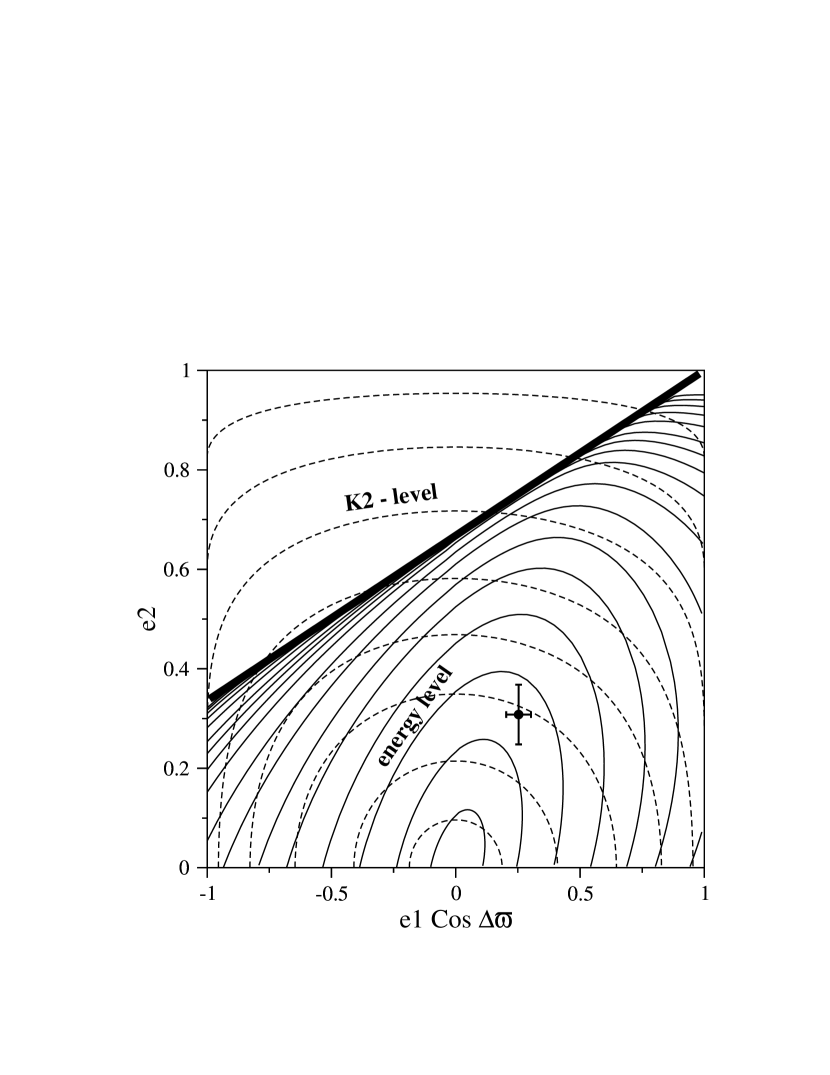
Figure 1: Energy and $K_{2}$ – levels of the secular Hamiltonian given by Eq. (4) on the ($e_{1}$,$e_{2}$) representative plane of initial conditions. The energy decreases whereas $K_{2}$ increases with increasing $|e_{1}\cos\Delta\varpi|$ and $e_{2}$. The signs + or –, preceding the variable $e_{1}\cos\Delta\varpi$, indicate that the initial values of $\Delta\varpi$ are zero or $180^{\circ}$, respectively. In constructing the level curves, we adopted the following values for the parameters: planet mass ratio $m_{1}/m_{2}=0.483$ and semimajor axes ratio $a_{1}/a_{2}=0.332$ (corresponding to those of the $\upsilon$ Andromedae planets C and D). The empty region above the thick line is the domain of crossing planetary orbits. The initial conditions of the $\upsilon$ Andromedae system in this plane is indicated by a full circle symbol; nominal 20% uncertainties are indicated for the eccentricities by error-bars.

Figure 1 shows the levels curves of the energy and AMD (hereafter denoted as $K_{2}$–levels) on the ($e_{1}$,$e_{2}$) representative plane. These level curves were constructed using the parameters of the $\upsilon$ Andromedae system of planets C and D (assuming edge-on coplanar orbits). The energy levels are shown by solid lines, whereas the $K_{2}$–levels are shown by dashed lines. The domain above the thick line at high eccentricities is the region where the planetary orbits cross each other; since there are no mechanisms which can protect the planets from close approaches between them (in contrast with the case of mean motion resonances), this domain was excluded from our studies. Finally, the location of the $\upsilon$ Andromedae system (planets C and D) is shown by a full circle, with uncertainties of 20% for the planetary eccentricities.

The structure of the energy levels is independent of the planetary masses; it depends upon only the ratio of the semi-major axes, $a_{1}/a_{2}$. Indeed, as can be seen in Eq. (4), the secular energy is directly proportional to the product of the planetary masses and the gravitational constant. Since the term $1/\Delta$ in the direct part of the disturbing function $R$ is independent of planetary masses and the indirect part does not contain secular terms, the secular energy can be normalized by the factor $\frac{Gm_{1}m_{2}}{a_{2}}$. Then the normalized secular energy, and thereby the structure of the energy levels, does not depend on the individual values of the semimajor axes, but depends only on the ratio, $a_{1}/a_{2}$.

The geometry of the $K_{2}$–levels, however, depends on both the semimajor axes and the masses. From the expression for $K_{2}$ given by Eq. (3), we can see that a natural normalization factor for this parameter is the constant $L_{2}$. This normalization reduces the semimajor axes dependence to only on the ratio, $a_{1}/a_{2}$. The mass dependence of $K_{2}$ goes as $\sim{m_{1}\over m_{2}}({M+m_{2}\over M+m_{1}})^{1/2}$. Therefore, for $m_{i}\ll M$, in the first order mass approximation, the mass dependence of $K_{2}$ can be reduced to only on the mass ratio of the planets, $m_{1}/m_{2}$. For example, in the $\upsilon$ Andromedae system, the planetary masses are of order $10^{-3}$ (in units of the stellar mass), and the first-order approximation works sufficiently well in this case. On the other hand, in the case of a binary stellar system with one planet, for example, where the mass of the companion is comparable to the mass of the central star, this approximation is not valid. For the calculations presented in this paper, we do not make this approximation, but rather adopt the values of $M,m_{1},m_{2},a_{1},a_{2}$ of the $\upsilon$ Andromedae system stated in the last paragraph of section 2.1.

2.3 Geometrical pictures of the secular behavior

In this section, we proceed with a qualitative study of the developed model and give a simple geometrical interpretation of the main features of secular motion. It should be emphasized that all information available from this study is obtained without integration of the equations of motion, Eq. (5). The study is based on the fact that the secular energy ${\overline{H}_{\rm sec}}$ and AMD (i.e. $K_{2}$) are both conserved along one secular path. This is reflected on the representative plane of initial conditions in the following way: Independent of whether the motion is circulation or oscillation of $\Delta\varpi$, an orbit generally passes twice through $\Delta\varpi=0$ or $180^{\circ}$. (The exceptional case of singular orbits and periodic orbits will be described below.) This means that an individual orbit is represented by two points on the ($e_{1}$,$e_{2}$)–plane: one point being the chosen initial condition, and the other point being its counterpart. Due to the energy and AMD conservation, the counterpart of one initial condition can be found easily as an intersection of the corresponding energy and $K_{2}$–levels.

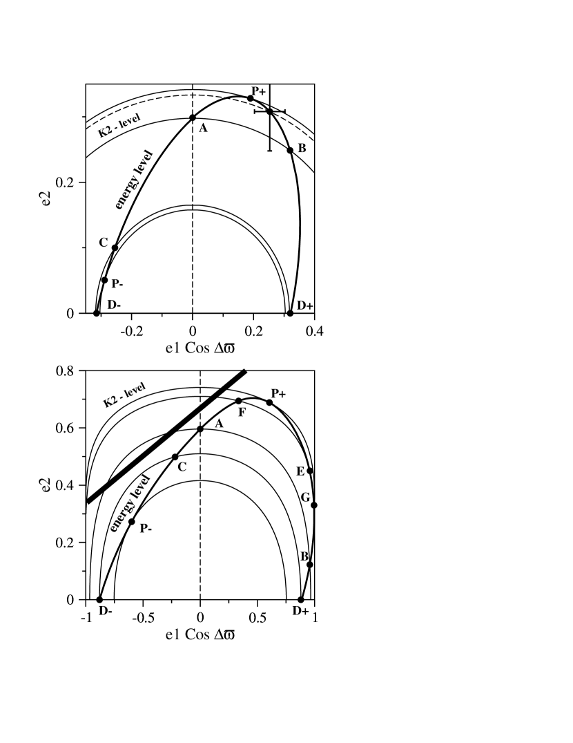
Figure 2: Top: Energy level with ${\overline{H}_{\rm sec}}=-0.41391$ (thick curve) and four characteristic $K_{2}$–levels (thin curves). The location of the current $\upsilon$ Andromedae system is indicated by a full circle symbol with 20% uncertainties error-bars. The points $P^{+}$ and $P^{-}$ show the location of oscillation centers, around zero and $180^{\circ}$, respectively. The initial conditions that correspond to oscillation around zero are situated on the energy segment between the points $A$ and $B$. Those with oscillation around $180^{\circ}$ between the points $C$ and $D^{-}$. Bottom: Energy level for ${\overline{H}_{\rm sec}}=-0.4295$, and the same four characteristic $K_{2}$ levels as in the top panel, plus an additional $K_{2}$–level which shows the location of a new libration center $E$ and its two counterparts, $F$ and $G$. Note the different scales of the axes in the two panels.

Figure 2 shows two representative ($e_{1}$,$e_{2}$)–planes of initial conditions which are identical to the plane shown in Fig. 1, except that only one energy level is plotted on each of them by thick curves. In the top panel, the energy level corresponds to the normalized secular energy of the “real” $\upsilon$ Andromedae system (${\overline{H}_{\rm sec}}=-0.41391$), while, in the bottom panel, it corresponds to a lower value ${\overline{H}_{\rm sec}}=-0.4295$. We will first concentrate our attention on the top panel. The location of the $\upsilon$ Andromedae system on the ($e_{1}$,$e_{2}$)–plane is shown by a full circle (20% uncertainties are indicated by error-bars). The $K_{2}$–level corresponding to the system is shown by a dashed curve. This $K_{2}$–level crosses the energy level at two points: one point is the initial condition marked by the full circle symbol, and other point is a counterpart of the first point. The two points belong to the same solution of the Hamiltonian system described by Eq. (4), and represent a quasi-periodic variation in the eccentricities and in $\Delta\varpi$. From the condition $K_{2}={\rm const}$, we can see that the secular oscillations of the eccentricities always occur with opposite phases: when the eccentricity of the outer planet $e_{2}$ is minimal, the eccentricity of the inner planet $e_{1}$ is maximal. Conversely, when the eccentricity $e_{2}$ is at a maximum, $e_{1}$ is at its minimum.

The qualitative behavior of the angular variable $\Delta\varpi$ also can be obtained from the geometrical analysis of the representative ($e_{1}$,$e_{2}$)–plane in Figure 2 top. Indeed, if both points of an orbital path are located at the positive right-hand side of the ($e_{1}$,$e_{2}$)–plane, the angle $\Delta\varpi$ oscillates around zero. Conversely, if both initial conditions are located at the negative left-hand side of the plane, $\Delta\varpi$ oscillates around $180^{\circ}$. Finally, when two initial conditions are at the opposite half–planes, the corresponding orbits of both planet are circulating with respect of the angle $\Delta\varpi$. The eccentricity of the more massive outer planet $e_{2}$ is minimal (consequently, $e_{1}$ is maximal), when $\Delta\varpi=0$, and is maximal ($e_{1}$ is minimal), when $\Delta\varpi=180^{\circ}$. In this way, from the geometrical picture presented in Figure 2 top, we can calculate the ranges of the eccentricity variation for both planets of the system under study.

The analysis of the geometry of the energy and $K_{2}$–levels on the ($e_{1}$,$e_{2}$)–plane described above is applied for any generic initial condition. However, for a given energy level, there are four characteristic $K_{2}$–levels which define the phase space structure and the qualitative character of the secular solutions. These are shown in Figure 2 top by continuous curves. The topmost $K_{2}$–level is tangent to the energy level at the point marked as $P^{+}$. The lowermost $K_{2}$–level has a minimum possible value and is tangent to the energy level at the point marked as $P^{-}$. These two $K_{2}$ levels represent extreme values of $K_{2}$ for the given energy level. The orbital solutions associated with these two extrema correspond to periodic solutions of the secular Hamiltonian system. These periodic orbits are characterized by constant values of the eccentricity and of $\Delta\varpi$.

The other two characteristic $K_{2}$–levels contain the initial conditions $e_{1}=0$ and $e_{2}=0$. One of these passes through the points $A$ and $B$ in Fig. 2 top and other one passes through the points $C$, $D^{+}$ and $D^{-}$. Note that, at $e_{2}=0$ the angular variable $\Delta\varpi$ is undefined. The points $D^{+}$ and $D^{-}$ both represent the initial condition $e_{2}=0$ on the ($e_{1}$,$e_{2}$) representative plane.

All initial conditions along a given energy level on the representative plane can be classified according to the motion of the corresponding angle $\Delta\varpi$. The periodic solution at point $P^{+}$ is characterized by zero amplitude oscillation. The orbits which start on the segment $AB$ of the energy level are characterized by oscillation of $\Delta\varpi$ around zero. The center of oscillation is the point $P^{+}$. The range of the eccentricity variation is given by the projections of the initial conditions on the corresponding axes. The periodic solution with zero amplitude oscillation around $180^{\circ}$ is at $P^{-}$. The orbits which start on the interval between $CD^{-}$ are oscillating around $180^{\circ}$. Once again, the planetary eccentricities vary in the range given by the projections of initial conditions on the corresponding axes. Finally, initial conditions in the intervals $CA$ and $BD^{+}$ correspond to circulating orbits with respect to $\Delta\varpi$.

Hereafter we designate the solutions near $P^{+}$ as Mode I and those near $P^{-}$ as Mode II. Near Mode I, the planetary apsidal lines are aligned, the secular angle $\Delta\varpi$ oscillates about $0$ and the planet eccentricities undergo small oscillations about the values of the Mode I periodic solution. Near Mode II, the apsidal lines are anti-aligned, $\Delta\varpi$ oscillates about $180^{\circ}$ and the planet eccentricities oscillate about the values of the Mode II periodic solution. Thus, the two modes describe two opposite stable ways of the planetary system to be aligned. Between the domains of Mode I and Mode II, there is a region of the phase space in which the motion of the angle $\Delta\varpi$ is a circulation. The secular oscillations of the planet eccentricities always occur with opposite phases. The eccentricities undergo secular variations in such way that, when $\Delta\varpi=0$, the eccentricity of the outer planet is minimal and one of the inner planet is maximal. Conversely, when $\Delta\varpi=180^{\circ}$, the eccentricity of the outer planet D is maximal and of the inner planet is minimal.

The bottom panel in Fig. 2 presents by the bold line the level curve of a lower secular energy. In this case, the domain covers higher eccentricities, and even eccentricities close to 1. All points $P^{+}$, $P^{-}$, $A$, $B$, $C$, $D^{+}$ and $D^{-}$ have the same interpretation as discussed above for the top panel. In addition, this figure exhibits a new feature which is the existence of a fifth characteristic $K_{2}$–level shown by points $E$, $F$, and $G$. The new $K_{2}$–level is tangent to the energy level at point $E$, and crosses it at points $F$ and $G$. This situation means that there is one orbit which crosses the $e_{1}\cos\Delta\varpi$ axis at three different points. To understand the behavior in this complicated case, we will need to integrate the equations of motion, Eq. (5); the results of the integrations are presented in the next section.

3 Secular Dynamics of the $\upsilon$ Andromedae system: Periodic and Ordinary Solutions; Nonlinear Secular Resonance

In this section, the insight gained by examining the geometrical structure of the levels on the representative plane is presented in quantitative form for the system of $\upsilon$ Andromedae planets C and D. Figure 3 shows the locations of periodic orbits and the various domains of oscillation or circulation of $\Delta\varpi$ in the ($e_{1}$,$e_{2}$)–plane of initial conditions, constructed for the parameters of this system. The detailed description and interpretation of this figure is as follows.

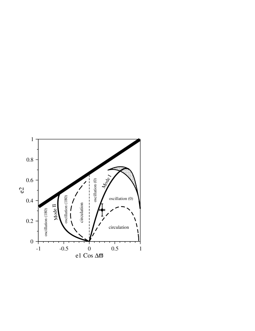
Figure 3: Periodic orbits and domains of oscillation and circulation in the ($e_{1}$,$e_{2}$)–plane of initial conditions, obtained for the parameters of the $\upsilon$ Andromedae system. The continuous thin curves plot the location of the stable periodic orbits: Mode I in the positive half–plane, Mode II in the negative half–plane. The domains of oscillation of $\Delta\varpi$ about $0$ (Mode I) and about $180^{\circ}$ (Mode II) are bounded by the dashed lines; the regions of circulation of $\Delta\varpi$ are also labeled. The shaded region at upper right is a family of unstable periodic orbits. The location of the current $\upsilon$ Andromedae system (planets C and D) is shown by the full circle symbol.

The upper boundary of the domain where the planetary orbits do not cross each other is shown by the thick line on the ($e_{1}$,$e_{2}$)–plane in Fig. 3. This curve is obtained from the simple geometrical condition of two crossing orbits, such as: $e_{2}=1-a_{1}(1-e_{1})/a_{2}$ and $e_{2}=a_{1}(1+e_{1})/a_{2}-1$, for $\Delta\varpi=0$, and $e_{2}=1-a_{1}(1+e_{1})/a_{2}$, for $\Delta\varpi=180^{\circ}$. Two families of stable periodic orbits are shown by the the thin continuous curves: one is located in the positive half–plane ($\Delta\varpi=0$), and other in the negative half–plane ($\Delta\varpi=180^{\circ}$). The two half–planes are separated by the dashed vertical line representing the initial condition $e_{1}=0$.

The periodic solutions of the Hamiltonian ${\overline{H}_{\rm sec}}$ given by Eq. (4) are defined by conditions:

$$\begin{array}[]{lcl}\dot{K}_{1}=-\frac{\partial{\overline{H}_{\rm sec}}}{\partial\Delta\varpi}=0{\rm,}&&\Delta\dot{\varpi}=\frac{\partial{\overline{H}_{\rm sec}}}{\partial K_{1}}=0{\rm.}\\ \end{array}$$ (7)

The Hamiltonian ${\overline{H}_{\rm sec}}$ is an even function of $\Delta\varpi$. Hence, the first of these equations provides immediately the trivial solution $\Delta\varpi=0\,\,({\rm mod}\,\,\pi)$, for non-vanishing $K_{1}$ and $K_{1}\neq K_{2}$. The second equation from Eq. (7) is solved numerically for the two cases, $\Delta\varpi=0$ and $\Delta\varpi=\pi$, and the condition $K_{2}={\rm const}$. The stability of the obtained periodic solutions is defined by the behavior of the Hessian matrix of ${\overline{H}_{\rm sec}}$ evaluated at the periodic orbit.

Recall that in linear secular theory, the general solutions are a linear superposition of two linear eigenmodes (e.g., Murray & Dermott, 1999). Our semi-numerical analysis yields the nonlinear generalization of the linear secular theory. In the positive half–plane of initial conditions in Fig. 3, the domain of Mode I, i.e. oscillation around zero, is defined by all initial conditions between the vertical line $e_{1}=0$ and the dashed curve. The domain below the dashed curve is of circulating orbits. The domain of Mode II is in the negative half–plane: the initial conditions for orbits oscillating around $180^{\circ}$ lie between the horizontal axis $e_{2}=0$ and the dashed curve. The domain to the right of the dashed curve and up to $e_{1}=0$ is of circulating orbits. In the limit of linear secular theory, the two modes would be represented in Fig. 3 by straight lines tangent at the origin to the continuous curves that are the nonlinear Modes I and II. It is clear that the departures from the linear secular theory become significant for $e_{1}\mathrel{\hbox to0.0pt{\lower 3.0pt\hbox{$\mathchar 536\relax$}\hss}\raise 2.0pt\hbox{$\mathchar 318\relax$}}0.3$. It is interesting to note that the nonlinearity is not symmetric for the two modes; it is especially severe for Mode II even at relatively small values of the eccentricity, $e_{2}\mathrel{\hbox to0.0pt{\lower 3.0pt\hbox{$\mathchar 536\relax$}\hss}\raise 2.0pt\hbox{$\mathchar 318\relax$}}0.1$.

Finally, the nonlinear analysis of the secular Hamiltonian yields a new feature not previously known, namely unstable periodic orbits at moderate-to-high eccentricities. In Fig. 3, these correspond to the boundaries of the shaded region near the upper right corner. These orbits were previously identified in Fig. 2 by the points $E$, $F$, and $G$. Their interpretation requires additional information, which we obtain by integration of the equations of motion Eq. (5). We describe this in more detail below, where we show that the shaded region in the ($e_{1}$,$e_{2}$)–plane represents a zone of nonlinear secular resonance, consisting of librating orbits bounded by an infinite-period separatrix.

The location of the current $\upsilon$ Andromedae system (planets $C$ and $D$) in the $e_{1},e_{2}$ plane of initial conditions is shown by the full circle symbol in Fig. 3. For the presently known best-fit planetary parameters, this system is within the Mode I domain with $\Delta\varpi$ oscillating about zero, as has been noted in previous studies (Chiang et al. 2001, Malhotra 2002, Chiang & Murray 2002).

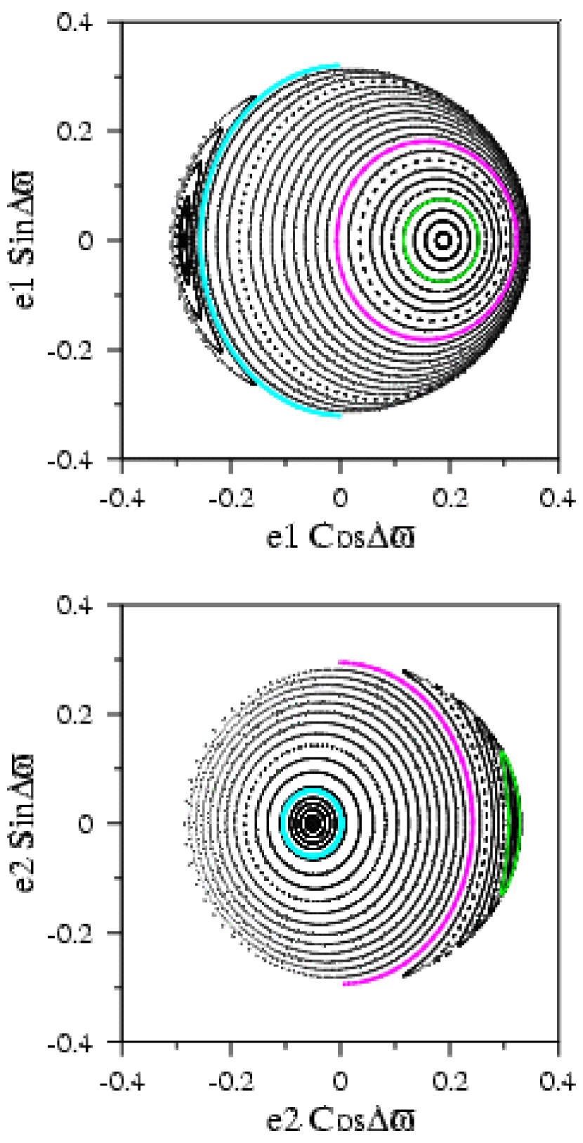
Figure 4: Secular phase space of the $\upsilon$ Andromedae planets C and D, at ${\overline{H}_{\rm sec}}=-0.41391$. Locations of the Mode I and Mode II are given by the fixed points on the top and bottom panels. The red and blue curves represent orbits passing through the $e_{1}=0$ and $e_{2}=0$ singularities of Eq. (5). The secular variations of the $\upsilon$ Andromedae planets C and D for the present best-fit initial conditions are shown by green curves (see text).

Figure 4 displays the solutions of the equations of secular motion, Eq. (5), in the two eccentricity planes, $(e_{i}\cos\Delta\varpi,e_{i}\sin\Delta\varpi)$. The top panel shows the secular variations of the inner planet and the bottom panel shows the secular variations of the outer planet. These solutions were obtained by numerical integration of a large set of initial conditions along the energy level corresponding to the $\upsilon$ Andromedae system (see top panel in Fig. 2). In each plane we see two fixed points, corresponding to the Mode I and Mode II periodic solutions. The $e_{1}$ plane is dominated by Mode I, whose fixed point lies in the central region; the Mode II fixed point lies near the left-hand boundary of the energy manifold. Conversely, in the $e_{2}$ plane, the Mode II periodic solution lies in the central region, while the Mode I periodic solution lies near the right-hand boundary of the energy manifold.

The smooth curves surrounding each of the two fixed points are periodic solutions of the reduced one-degree-of-freedom system, but quasi-periodic solutions of the full two-degrees-of-freedom secular system; as noted previously, we refer to these as simply quasi-periodic solutions. Note that even though the motion of the angle $\Delta\varpi$ may be either oscillation (about $0$ or $180^{\circ}$) or circulation, there is no separatrix associated with an unstable infinite-period solution. To better understand this feature, we plot by red and blue curves two particular solutions in Fig. 4. These solutions are associated with the singularities in Eqs. (5), which occur at $K_{1}=0$ and $K_{1}=K_{2}$ or, in the eccentricity notation, at $e_{1}=0$ and $e_{2}=0$. (As is well known, these are not physical singularities, but merely due to the choice of variables.) The solution shown by the red curve was obtained with initial condition $e_{1}\approx 0$ and is seen as a smooth curve passing through the origin in the $e_{1}$ plane (upper panel). In comparison, the solution obtained with initial condition $e_{2}\approx 0$ and shown by the blue curve, appears as the ‘false’ separatrix in the $e_{1}$ plane, separating the domains of different modes of motion. An analogous situation is seen in the $e_{2}$ plane (lower panel), where the blue curve is a smooth curve passing through the origin and the red curve separates the domains of two modes of motion. We emphasize that the boundary separating the oscillation of $\Delta\varpi$ about either 0 or $180^{\circ}$ is not a zero-frequency separatrix, but simply the quasiperiodic solutions that pass through the singular initial values, $e_{1}=0$ or $e_{2}=0$. The separatrix-like curves in Fig. 4 are owed to the effects of projecting the canonical solutions on to a plane of non-canonical variables; these are better visualized over a sphere (for more details, see Pauwels 1983).

Finally, the solution corresponding to the current best-fit initial conditions of the $\upsilon$ Andromedae planets $C$ and $D$ is shown by the green trajectories in Fig. 4. This solution oscillates about the Mode I periodic solution; the oscillation amplitude of $\Delta\varpi$ is 25^∘ about 0. Note, however, that the oscillation amplitude is quite sensitive to the initial conditions. This is most readily seen in the structure near the green curves in Fig. 4: small changes in initial conditions lead to large changes in the oscillation amplitude. A complete analysis of the observational uncertainties in the parameters of this system is beyond the scope of the present work. Suffice to note that these uncertainties (see Fig. 3) do not exclude significantly larger or significantly smaller amplitudes of oscillation of $\Delta\varpi$. For example, assuming all other parameters are fixed, the 20% nominal uncertainty in the eccentricities implies that the $\Delta\varpi$ oscillation amplitude may be as large as $70^{\circ}$ or as small as $9^{\circ}$. As we discuss in section 5, this uncertainty is problematic for theories of the origin of the large eccentricities.

Figure 5: Spectral map corresponding to the solutions shown on the planet C panel in Figure 4. The abscissas ($e_{1}\cos\Delta\varpi$) in the spectral map are the initial conditions at $\Delta\varpi=0$ and $\Delta\varpi=180^{\circ}$. The dashed line indicates the initial value of $e_{1}\cos\Delta\varpi$ of the ${\upsilon}$ Andromedae system.

Figure 5 shows the spectral map obtained from the Fourier analysis of solutions calculated with initial conditions on the horizontal axis on the planet C panel in Fig. 4 top. The map shows the frequency of all peaks present in the Fourier spectra of the eccentricities $e_{1}$ and $e_{2}$ that are clearly above noise level (arbitrarily defined as 20 per cent of the largest spectral peak). Besides the discussion above about the nature of the solutions separating the oscillation zones, one may note the continuous evolution of the frequencies on the corresponding spectral map. The map shows only one frequency and its higher harmonics that is characteristic of one-degree of freedom dynamical systems. The continuous smooth evolution of frequency through the domain of initial conditions does not exhibit the typical signature of a separatrix associated with an unstable periodic orbit. The range of the variation of the period of $\Delta\varpi$ is between 6,500 and 10,000 years: the shortest period occurs when the system is near Mode I and the longest period occurs near Mode II. The initial co-ordinate of the ${\upsilon}$ Andromedae system (planets C and D) is indicated by the dashed vertical line; the oscillation period of $\Delta\varpi$ in this case is $\sim 7,100$ years.

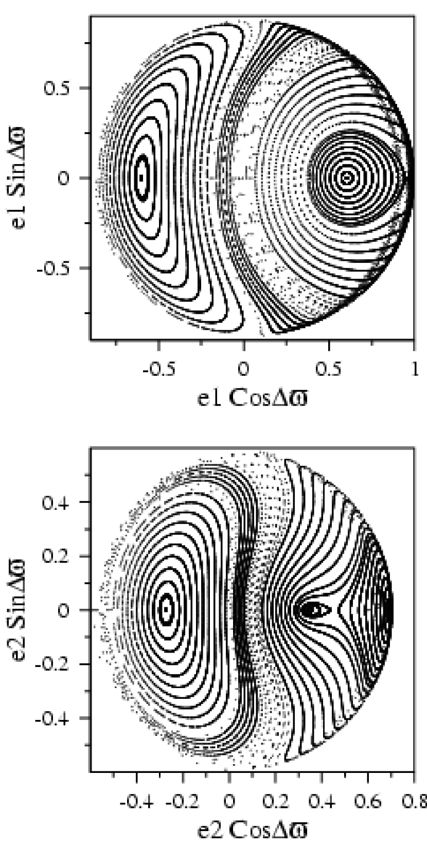
Figure 6: Same as in Figure 4, but for ${\overline{H}_{\rm sec}}=-0.4295$. The erratic scatter of the points at eccentricities close to 1 is due to the loss of numerical accuracy.

Figures 6 and 7 are analogous to Figures 4 and 5, respectively, except they were obtained for the lower value of the normalized secular energy, ${\overline{H}_{\rm sec}}=-0.4295$. For this lower energy, we find that a qualitatively new feature appears in the phase space. In Fig. 6, we see the formation of a new libration center and one saddle-point in the domain of high eccentricities, where the effect of nonlinearity of the secular perturbations is strong. This feature can be associated with the advent of a nonlinear secular resonance zone, which is bounded by a zero-frequency separatrix and which occupies the domain about the Mode I fixed point at large eccentricities. This feature can be identified in the spectral map shown in Fig. 7, where the $\Delta\varpi$–frequency tends to $0$ at $e_{1}\cos\Delta\varpi=0.36$.

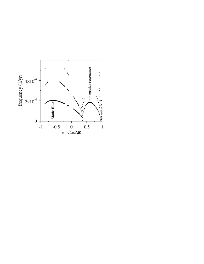
Figure 7: Same as in Figure 5, but for ${\overline{H}_{\rm sec}}=-0.4295$.

4 Dependence on the Planetary Masses and Semimajor Axes Ratios

In the previous sections, we have analyzed the secular behavior for one set of values the planetary mass and semimajor axis ratios: $a_{1}/a_{2}=0.332$ and $m_{1}/m_{2}=0.461$, values which are pertinent to the current ${\upsilon}$ Andromedae planetary system. In this section, we will vary these two parameters and see the effect on the secular phase space structure. To see this dependence, we will plot the locations of periodic orbits and the domains of circulation or oscillation of $\Delta\varpi$ in the ($e_{1}$,$e_{2}$) representative plane of initial conditions. We will first consider the case when the outer planet is equal or more massive than inner one, that is $m_{1}/m_{2}\leq 1$. Fixing the inner mass at $m_{1}=1.83M_{\rm Jup}$, we take three values of the outer mass: $m_{1}/m_{2}=1/1$, $m_{1}/m_{2}=1/2$ and $m_{1}/m_{2}=1/4$. Also, fixing the inner semimajor axis at $a_{1}=0.83\,{\rm AU}$, we take three values of the outer semi-major axis: $a_{2}=1.5\,{\rm AU}$, $a_{2}=2.5\,{\rm AU}$ and $a_{2}=5\,{\rm AU}$.

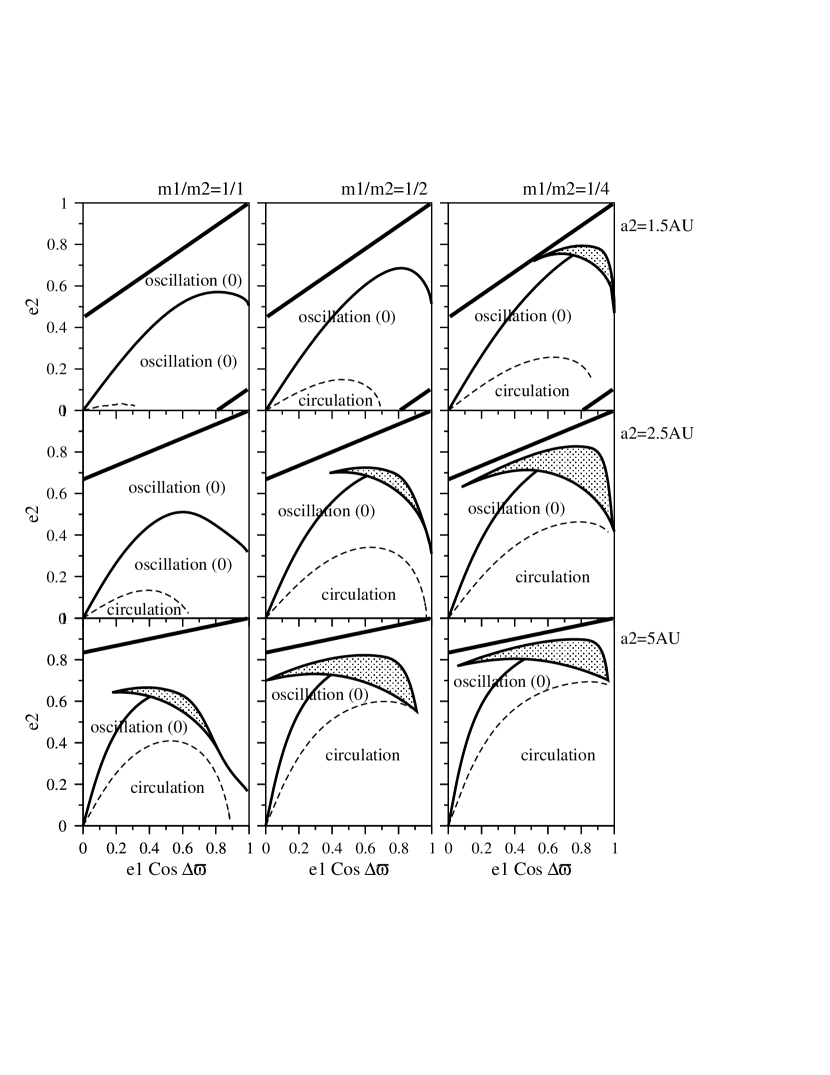
Figure 8: Periodic orbits and domains of oscillation and circulation of $\Delta\varpi$ in the representative ($e_{1}$,$e_{2}$)–planes, for a range of planetary masses and semimajor axes. Rows: a fixed value of the inner semi-major axis $a_{1}=0.83\,{\rm AU}$ and three values of the outer semi-major axis: $a_{2}=1.5\,{\rm AU}$ (top), $a_{2}=2.5\,{\rm AU}$ (middle) and $a_{2}=5\,{\rm AU}$ (bottom); Columns: a fixed value of the inner mass $m_{1}=1.83M_{\rm Jup}$ and three values of the outer mass, such as: $m_{1}/m_{2}=1$ (left), $m_{1}/m_{2}=1/2$ (middle) and $m_{1}/m_{2}=1/4$ (right). The shaded regions are domains of the nonlinear secular resonance.

The results are shown in Fig. 8, where the rows present the variation with mass parameter, for a fixed value of $a_{1}/a_{2}$, while the columns present the variation with axis parameter, for a fixed value of $m_{1}/m_{2}$. Since the most significant changes occur at $\Delta\varpi=0$, only positive half–planes are presented in Fig. 8. In each plane, the boundaries of the domain of non-crossing planetary orbits are shown by thick inclined lines. The families of stable periodic orbits are shown by continuous black curves, whereas the boundaries of domains of $\Delta\varpi$–oscillation are shown by dashed curves. Finally, the domains of the secular resonance are shown as shaded regions on the ($e_{1}$,$e_{2}$)–planes. Note that the parameters (planet mass and semimajor axis ratios) used in construction of the mid-row and mid-column are very close to those of the current ${\upsilon}$ Andromedae system shown in Fig. 3.

Figure 8 gives a global view of all possible regimes of motion with respect to the secular angle $\Delta\varpi$. When the planetary masses are equal and the mutual distances are small, almost the whole phase space of the system is oscillations of the angle $\Delta\varpi$ around 0. In this case, as can be easily inferred from the geometrical pictures in Fig. 2, the oscillations of $\Delta\varpi$ around $180^{o}$ will cover almost the whole negative half–plane of initial conditions (not shown here). The circulation occurs only in the domains of small eccentricities. With increasing mutual distance of the planets, the regions of circulation are also increasing. The same effect is observed when the mass of the outer planet increases. The secular resonance seems to be a common feature of the planetary system, particularly, when the masses and axes ratios are not close to 1. Its location on the ($e_{1}$,$e_{2}$) representative plane of initial conditions is always in the regions of the very-high eccentricities of the more massive outer planet. The orbit of the inner planet in this case can be nearly circular.

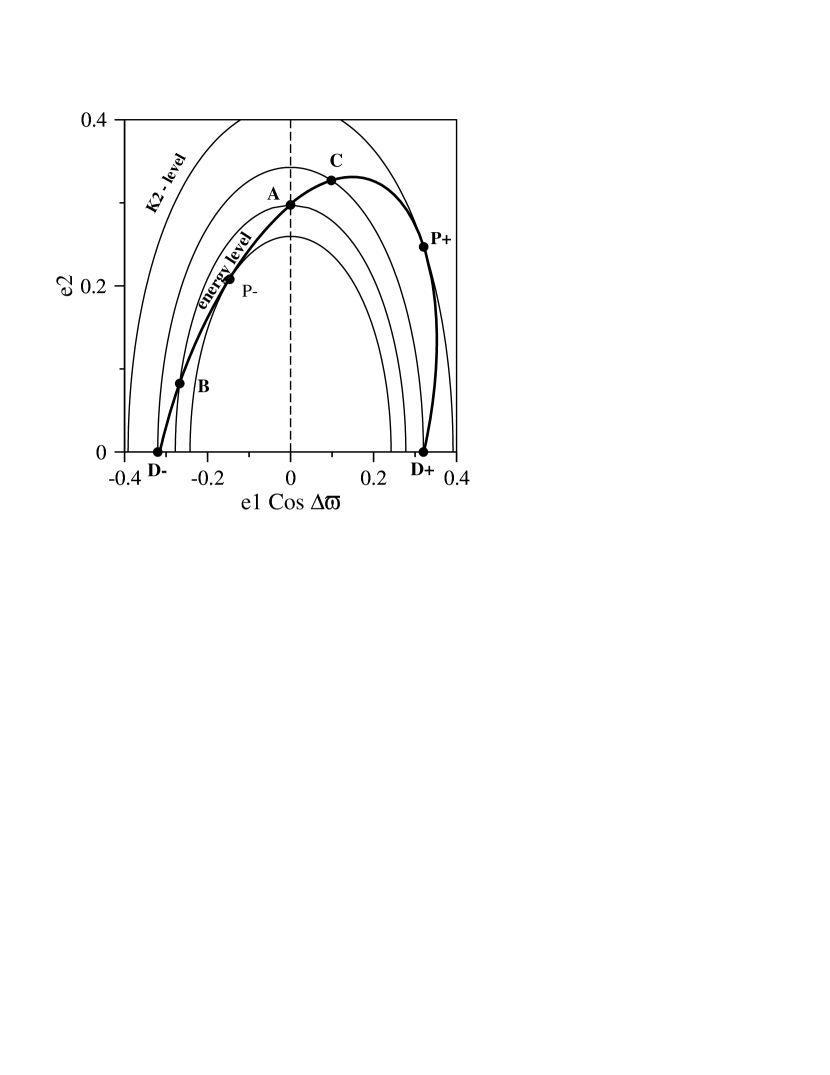
Figure 9: Same as in Figure 2, but calculated with $m_{1}=3.97M_{\rm Jup}$ and $m_{2}=1.83M_{\rm Jup}$.

Now we will consider the case when mass of the inner planet is larger that the mass of the outer planet, that is $m_{1}/m_{2}>1$. The geometrical picture of the ($e_{1}$,$e_{2}$) representative plane of initial conditions corresponding to this case is shown in Fig. 9. This plane was constructed with the same axes ratio used in Fig. 3, but the planetary masses were changed to $m_{1}=3.97M_{\rm Jup}$ and $m_{2}=1.83M_{\rm Jup}$. Since the axes ratio has not been changed, the energy level shown by the thick curve is the same level, $H_{sec}=-0.41391$, shown in Fig. 2. However, the structure of the $K_{2}$–levels is different when compared to those in Fig. 3 because of the mass dependence of the variable $K_{2}$. The main geometrical difference is the location of the points B and C on the ($e_{1}$,$e_{2}$)–plane: now the point B is located in the negative half–plane and the point C in the positive half–plane. This means that the oscillation of $\Delta\varpi$ around $0$ occurs along the energy segment ${\bf CD^{+}}$ and around $180^{\circ}$ along the energy segment ${\bf AB}$. Finally, the initial conditions chosen in the intervals $CA$ and $BD^{-}$ correspond to circulating orbits with respect to $\Delta\varpi$.

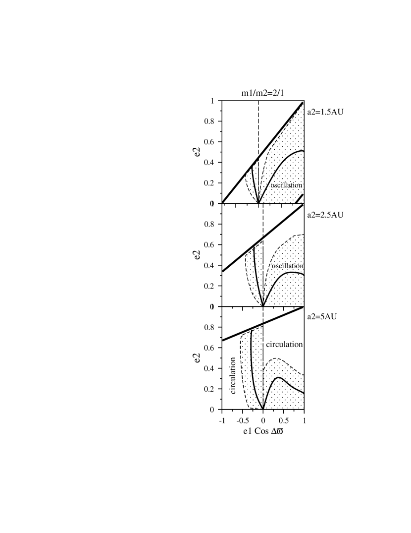
Figure 10: Same as in Figure 8, but for $m_{1}=3.97M_{\rm Jup}$ and $m_{2}=1.83M_{\rm Jup}$. The shaded regions are domains of oscillations of $\Delta\varpi$ around $0$ or $180^{o}$.

The dependence of the secular behavior on the semimajor axes ratio in the case of $m_{1}/m_{2}=2$ is shown in Fig. 10. This figure is similar to Fig. 8: it was constructed using the same three values of the outer semi-major axis $a_{2}=1.5\,{\rm AU}$, $a_{2}=2.5\,{\rm AU}$ and $a_{2}=5\,{\rm AU}$, whereas the inner semimajor axis was fixed at $a_{1}=0.83\,{\rm AU}$. As in Figure 8, the boundaries of the domain of noncrossing planetary orbits are shown by the thick inclined lines on each panel. The families of stable periodic orbits are shown by the thin continuous curve, whereas the boundaries of domains of $\Delta\varpi$–oscillation are shown by the dashed curves. The main difference in the secular motion is that in this case the periodic orbits have lower values of $e_{2}$ compared to the case with $m_{1}/m_{2}=1/2$, and the nonlinear secular resonance zone does not occur for all considered values of the axes ratio. Interestingly, the location of Mode I in this case is remarkably different from that predicted by linear secular theory.

5 Summary and Discussion

The nonlinear secular perturbation analysis of the planar three body (two planet) problem presented here has been motivated by the recent discovery of extra-solar planetary systems which have large orbital eccentricities and, in some cases, exhibit secular oscillations of their apsidal lines. The classical Laplace-Lagrange linear secular perturbation theory is insufficient for the precise analysis of such systems. We developed a semi-analytical approach, consisting of a numerical averaging over the short-period perturbations in the mutual interaction of the two planets to obtain the secular Hamiltonian. The Hamilton-Jacobi approach we use shows that the secular Hamiltonian is separable. (It is reducible to a one-degree-of-freedom integrable dynamical system for the canonical coordinate $\Delta\varpi$.) We obtain the periodic orbits of this system, and we present a geometrical picture of the secular phase space of the two-planet system in terms of physical variables, the eccentricities and periastron longitudes. This phase space structure depends upon two parameters: the ratios of the planets’ masses and their semimajor axes. The description of the secular variations of the system is completed by the initial conditions: the eccentricities and the relative longitude of the periastrons. Owing to the symmetries in the secular Hamiltonian, the phase space structure can be visualized in a two dimensional representative plane of initial conditions, $e_{2}$ and $e_{1}\cos\Delta\varpi$, where initial $\Delta\omega$ is either 0 or $180^{\circ}$.

The locations of periodic orbits and the domains of different quasiperiodic motions (corresponding to the stationary solutions and oscillations or circulations of $\Delta\varpi$) are then easily obtained in this plane of initial conditions, for given values of the parameters ($m_{1}/m_{2},a_{1}/a_{2}$). As expected from the linear secular perturbation theory for two planets, there exist two families of stable periodic orbits which describe the aligned and anti-aligned orientations of the two planets’ apsidal lines. Departures from the linear secular theory are readily visualized in this plane of initial conditions. In the domain of large eccentricities, we find a new feature which consists of a family of unstable periodic orbits. In this regime, the secular phase space contains a nonlinear resonance zone bounded by a zero-frequency separatrix. We emphasize that all of these results are obtained by means of a geometrical analysis based on the global constants of motion, and without time-expensive numerical integrations of the equations of motion.

We applied this analysis to the specific case of the system of two outer planets, C and D, of $\upsilon$ Andromedae, assuming edge-on co-planar orbits. We find that the nonlinear effects are significant in this case for eccentricities exceeding $\sim 0.3$ in the neighborhood of the aligned mode, and $\sim 0.1$ in the neighborhood of the anti-aligned mode. As noted already in previous studies of the dynamics of this system, the present best-fit initial conditions place this system in the domain of oscillations about the periodic orbit describing the aligned mode (Mode I, $\Delta\varpi=0$). Our analysis shows that the secular behavior of the $\upsilon$ Andromedae system is stable over a large domain of initial eccentricities. On the representative plane of initial conditions, the domain of stable motion has an upper bound at the collision curve defined by close approaches between two planets; below the collision curve, a secular instability occurs in the vicinity of the nonlinear secular resonance located near $e_{1}=0.6$ and $\Delta\varpi=0$ (Fig. 3).

We have presented an analysis of the secular dynamics of the three-body planetary system over a wide range of the planetary mass and semimajor axis ratios. The systems always exhibit two main regimes of motion, characterized by circulation of $\Delta\varpi$ or its oscillation around 0 or $180^{\circ}$. The existence of a third regime, the nonlinear secular resonance, depends on the values of the physical parameters. For example, when the planetary masses are equal and their mutual distances are small, the nonlinear secular resonance does not occur; however, under these conditions, the probability of finding the system in the oscillation (around 0 or $180^{\circ}$) regime of motion is very close to 1. When both mass and semimajor axis ratios are far from 1, the domains of oscillation of $\Delta\varpi$ decrease, and the nonlinear secular resonance zone appears. The secular resonance feature discovered in our nonlinear analysis is presently only a theoretical curiosity, as no real system is known which can be associated with this dynamical state. However, the regime of planetary parameters where this feature is significant is not especially extreme, and it would not be surprising if such systems are identified in the future.

The origin of the high planetary eccentricities of the $\upsilon$ Andromedae planets C and D, as well as of many other exo-planetary systems, are an outstanding problem of high current interest. Two basic physical mechanisms that have been proposed to account for the high eccentricities invoke dynamical planet-planet interactions (Ford et al. 2001, Marzari & Weidenschilling 2002) or planet-disk interactions (Goldreich & Sari 2003); more complex scenarios involving planet-disk interactions moderated by resonant interactions between two planets have also been suggested (Chiang et al. 2002, Lee & Peale 2002, Malhotra 2002, Chiang & Murray 2002). It has been pointed out that in some multiple-planet systems the occurrence of apsidal oscillation, and especially the amplitude of that oscillation, may serve to constrain the physical mechanisms (Malhotra 2002). Unfortunately, the observational uncertainties of the planetary parameters of even the best-known exo-planetary system, $\upsilon$ Andromedae, are still too large to define sufficiently precisely the amplitude of oscillation of $\Delta\varpi$, and thus to favor one scenario over another. We await future improvements in the accuracy of the parameters of this system and others to more precisely determine their dynamics and thereby constrain their dynamical history.

The method developed here is a non-linear generalization of the classical secular perturbation theory for the planar three body problem. In future work we hope to extend this to non-coplanar systems, and to apply the analysis to the secular dynamics of other planetary systems. We note that the Hamilton-Jacobi approach used here also provides a powerful means to explore the effects of adiabatic evolution of the energy and angular momentum due to dissipative interactions with the nascent protoplanetary disk, identify adiabatic invariants, and thus possibly obtain additional insights into the dynamical history of some exo-planetary systems.

REFERENCES

• Brouwer, D., and G.M. Clemence 1961. Methods of Celestial Mechanics. Academic Press, New York and London.

• Chiang, E.I., S. Tabachnik, and S. Tremaine 2001. Apsidal Alignment in ${\upsilon}$ Andromedae. AJ 122, 1607-1615.

• Chiang, E.I., D. Fischer, and E. Thommes 2002. Excitation of Orbital Eccentricities of Extrasolar Planets by Repeated Resonance Crossings. ApJ 564, L105-L109.

• Chiang, E.I., and N. Murray 2002. Eccentricity Excitation and Apsidal Resonance Capture in the Planetary System ${\upsilon}$ Andromedae. ApJ 576, 473-477.

• Ford, E.B., 2003. Quantifying the uncertainty in the orbits of extra-solar planets, AJ, submitted (preprint: astro-ph/0305441).

• Ford, E.B., M. Havlikova, and F.A. Rasio 2001. Dynamical instabilities in extrasolar planetary systems containing two giant planets. Icarus 150, 303.

• Goldreich, P., and R. Sari 2003. Eccentricity Evolution for Planets in Gaseous Disks. ApJ 585, 1024-1037.

• Laplace, P.S. 1799. “Mécanique Céleste”. English translation by N. Bowditch, Chelsea Pub. Comp. Edition, N.Y., 1966.

• Laskar, J., and P. Robutel 1995. Stability of the planetary three-body problem: I. Expansion of the planetary Hamiltonian. Celest. Mech. Dynam. Astron. 62, 193-217.

• Laskar, J. 2000. On the Spacing of Planetary Systems. Physical Review Letters 84, 3240-3243.

• Lee, M.H., and S.J. Peale 2002. Dynamics and Origin of the 2:1 Orbital Resonances of the GJ 876 Planets. ApJ 567, 596-609.

• Malhotra, R. 1998. Orbital resonances and chaos in the Solar System. In Solar System Formation and Evolution ASP Conference Series (D.Lazzaro et al., Eds.) 149, 37-63.

• Malhotra, R. 2002. A Dynamical Mechanism for Establishing Apsidal Resonance. ApJ 575, L33-L36.

• Marzari, F., and S.J. Weidenschilling 2002. Eccentric Extrasolar Planets: The Jumping Jupiter Model. Icarus 156, 570-579.

• Michtchenko, T. and S. Ferraz-Mello 2001. Modeling the 5:2 mean-motion resonance in the Jupiter-Saturn planetary system. Icarus 149, 357-374.

• Murray, C.D., and S.F. Dermott 1999. Solar System Dynamics. Cambridge University Press, 274-279.

• Pauwels, T. 1983. Secular orbit-orbit resonance between two satellites with non-zero masses. Celest. Mech. 30, 229-247.

• Poincaré, H. 1897. Sur une forme nouvelle des équations du problème des trois corps. Bull.Astron. 14, 53-67.

• Stepinski, T. F., R. Malhotra, and D.C. Black 2000. The $\upsilon$ Andromedae System: Models and Stability. ApJ 545, 1044-1057.

• Yuasa, M., and G. Hori 1979. New approach to the planetary theory. In Dynamics of the Solar System (R.L. Duncombe, Ed.), D.Reidel, Dordrecht, 69-73.