WMAP and Supergravity Inflationary Models

Abstract

We study a class of $N=1$ Supergravity inflationary models in which the evolution of the inflaton dynamics is controlled by a single power in the inflaton field at the point where the observed density fluctuations are produced, in the context of the braneworld scenario, in light of WMAP results. In particular, we find that the bounds on the spectral index and its running constrain the parameter space both for models where the inflationary potential is dominated by a quadratic term and by a cubic term in the inflaton field. We also find that $\alpha_{s}>0$ is required for the quadratic model whereas $\alpha_{s}<0$ for the cubic model. Moreover, we have determined an upper bound on the five-dimensional Planck scale, $M_{5}\mathrel{\hbox to0.0pt{\lower 4.0pt\hbox{\hskip 1.0pt$\sim$}\hss}\raise 1.0pt\hbox{$<$}}0.019$ M, for the quadratic model. On the other hand, a running spectral index with $n_{s}>1$ on large scales and $n_{s}<1$ on small scales is not possible in either case.

I Introduction

The first year WMAP data has confirmed the “concordance” values of the cosmological parameters with unprecedented accuracy and given important information on the primordial spectrum of density perturbations Bennet ; Spergel . Their results favor gaussian, purely adiabatic fluctuations and a spectral index that runs from $n_{s}>1$ on large scales to $n_{s}<1$ on small scales. Moreover, WMAP has confirmed earlier COBE DMR observations that there is a lower amount of power on the largest scales when compared to that predicted by the standard $\Lambda$CDM models.

Although these results are not yet firmly established (for an analysis of WMAP results which finds no evidence of running see Ref. BargerSeljak ), it seems worthwhile to reexamine inflationary models in light of WMAP results, as they may give us further insight into the very early universe. Supergravity inflationary models are particularly important as supersymmetry (or its local version, supergravity) is the only known way to avoid the hierachy problem, i.e. the fact that the high energy scale of inflation communicates to other sectors of the theory driving the electroweak scale much above its observed value via radiative corrections.

However, supergravity inflationary models also suffer from a kind of hierarchy problem as supersymmetry is broken by the large cosmological constant during inflation giving all scalars, including the inflaton, a soft mass of the order of the Hubble parameter Bertolami . As a result, the curvature of the inflaton potential, as measured by the $\eta$ slow-roll parameter, becomes too large to allow for a sufficiently long period of inflation to take place - the so-called $\eta$ problem.

Recently, it has been shown that this problem can be avoided within the Randall-Sundrum Type II braneworld scenario Randall , at least for a class of supergravity models in which the evolution of the inflaton dynamics is controlled by a single power at the point where the observed density fluctuations are produced and the inflationary potential can, therefore, be approximately given by

$$V\simeq\Delta^{4}\left[1+c_{n}\left(\phi\over M\right)^{n}\right]~{}~{},$$ (1)

where $M=M_{P}/\sqrt{8\pi}$ is the reduced Planck mass. In the braneworld context, the Friedmann equation acquires an additional term quadratic in the energy density Binetruy

$$H^{2}={8\pi\over 3M_{P}^{2}}\rho\left[1+{\rho\over 2\lambda}\right]~{},$$ (2)

where $\lambda$ is the brane tension, which relates the four and five-dimensional Planck scales through

$$M_{P}=\sqrt{{3\over 4\pi}}{M_{5}^{3}\over\sqrt{\lambda}}~{}~{}.$$ (3)

It is precisely the new parameter $M_{5}$ that plays a crucial role in the resolution of the $\eta$-problem in supergravity inflation. As shown in Ref. Bento2 , for the case where the first term in Eq. (1) is dominant and $n=2$ or $n=3$, this problem can be avoided provided the five-dimensional Planck mass satisfies, respectively, the condition $M_{5}\mathrel{\hbox to0.0pt{\lower 4.0pt\hbox{\hskip 1.0pt$\sim$}\hss}\raise 1.0pt\hbox{$<$}}10^{16}~{}\mbox{GeV}$ and $M_{5}\simeq 1.1\times 10^{16}~{}\mbox{GeV}$. The case where the second term is dominant and $n=2$, corresponding to chaotic inflation, has been studied in Refs. Maartens ; Bento1 , where it is shown that it is possible to achieve successful inflation with sub-Planckian field values, thereby avoiding well known difficulties with higher order non-renormalizable terms.

In this paper, we reexamine this class of supergravity models for the quadratic and cubic cases in light of WMAP results. The case of chaotic inflation has already been analysed in Ref. Liddle1 , with the conclusion that the quadratic potential is allowed at two-sigma for any value of the brane tension and the quartic potential is very constrained, particularly in the case where the inflationary energy scale is close to the brane tension. Here we concentrate on the case where the first term in Eq.  (1) is dominant. We find that although the running of the scalar spectral index is within the bounds determined by WMAP for both the quadratic and cubic models and for a wide range of potential parameters, a spectral index running from $n_{s}>1$ on large scales to $n_{s}<1$ on small scales is not possible in either case as precisely the opposite trend is found.

II Quadratic potential

We first consider the case where the potential is quadratic in the inflaton field, $\phi$, and we rewrite it as

$$V=V_{0}+{1\over 2}m^{2}\phi^{2}~{}~{},$$ (4)

and assume that the first term is dominant.

In supergravity, effective mass squared contributions of fields are given by

$${1\over 2}m^{2}=8\pi{V_{0}\over M_{P}^{2}}\approx 3H^{2}~{},$$ (5)

since the horizon of the inflationary De Sitter phase has a Hawking temperature given by $T_{H}=H/2\pi$ Bertolami .

Contributions like the ones of Eq. (5) lead to $\eta\equiv M_{P}^{2}V^{\prime\prime}/8\pi V\simeq 2$ ; however, the onset of inflation requires $\eta\ll 1$. Within the braneworld scenario, however, $\eta$ and the remaining “slow-roll” parameters $\epsilon$ and $\xi$, are modified, at high energies, by a factor proportional to $\lambda/V$ Maartens

$$\epsilon \equiv {M_{P}^{2}\over 16\pi}\left({V^{\prime}\over V}\right)^{2}{1+{V/\lambda}\over(1+{V/2\lambda})^{2}}~{}~{},$$ (6)

$$\eta \equiv {M_{P}^{2}\over 8\pi}\left({V^{\prime\prime}\over V}\right){1\over 1+{V/2\lambda}}~{}~{},$$ (7)

$$\xi \equiv {M_{P}^{4}\over(8\pi)^{2}}{V^{\prime}V^{\prime\prime\prime}\over V^{2}}{1\over(1+V/2\lambda)^{2}}.$$ (8)

In the high energy approximation, $V\gg\lambda$, we obtain, for this model

$$\epsilon = {M_{P}^{2}\over 8\pi}{m^{4}\phi^{2}\over V_{0}^{2}\alpha}~{},$$ (9)

$$\eta = {4\over{\alpha}}~{},$$ (10)

$$\xi = 0~{},$$ (11)

where we have also used the approximation $V\simeq V_{0}$ during inflation and the definition $\alpha\equiv V_{0}/\lambda$. As shown in Ref. Bento2 , if $\alpha$ is sufficiently large, the $\eta$-problem is automatically solved by the brane correction.

The number of $e$-folds during inflation, $N$, in the braneworld scenario, is given by Maartens

$$N\simeq-{8\pi\over M_{P}^{2}}\int_{\phi_{I}}^{\phi_{F}}{V\over V^{\prime}}\left[1+{V\over 2\lambda}\right]d\phi~{}~{},$$ (12)

in the slow-roll approximation. We see that, as a result of the modification in the Friedmann equation, the expansion rate is increased, at high energies, by a factor $V/2\lambda$. For this model, we get, in the high-energy approximation,

$$N= {\alpha\over 4}\log\left({\phi_{I}\over\phi_{F}}\right)+{2\pi\alpha\over M_{P}^{2}}(\phi_{I}^{2}-\phi_{F}^{2})$$ (13)

$$+{16\pi^{2}\alpha\over M_{P}^{4}}(\phi_{I}^{4}-\phi_{F}^{4})~{}.$$

Notice that, for sub-Planckian field values, the second and third terms are negligible. The value of $\phi$ at the end of inflation can be obtained from the condition

$${\rm max}\{\epsilon(\phi_{F}),|\eta(\phi_{F})|\}=1~{}~{}.$$ (14)

However, we shall consider $\phi_{F}=\beta M$ as a free parameter since quadratic potentials of the type we are studying arise typically in the context of hybrid inflation, once some other field is held at the origin by its interaction with $\phi$. In these scenarios, inflation may end due to instabilities triggered by the dynamics of the other field and, therefore, the amount of inflation strongly depends on the value of the inflaton field at the end of inflation, $\phi_{F}$, at the time the instabilities arise. Actually, these instabilities are necessary in order to end inflation as $\epsilon\ll 1$ for $\alpha\gg 1$ and sub-Planckian field values.

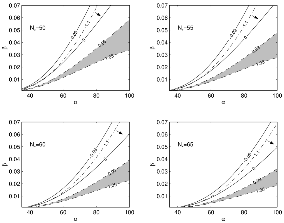
Figure 1: Contours of the inflationary observables $n_{s}$ (dashed), $\alpha_{s}$ (full) and $r_{s}$ (dot-dashed) in the ($\alpha,\beta$) plane for the quadratic model; the arrow points the direction of decreasing $r_{s}$. The allowed region is shaded and, as indicated, different panels correspond to different values of $N_{\star}$.

The amplitude of scalar perturbations is given by Maartens

$$A_{s}^{2}\simeq\left.\left({512\pi\over 75M_{P}^{6}}\right){V^{3}\over V^{\prime 2}}\left[1+{V\over 2\lambda}\right]^{3}\right|_{k=aH}~{}~{},$$ (15)

where the right-hand side should be evaluated as the comoving wavenumber equals the Hubble radius during inflation, $k=aH$. Thus the amplitude of scalar perturbations is increased relative to the standard result at a fixed value of $\phi$ for a given potential. Using the high energy approximation and $V\simeq V_{0}$ in Eq. (15), we obtain

$$A_{s}^{2}\simeq{1600\pi\over 75}{V_{0}^{6}\over\lambda^{3}m^{4}}\exp\left(-8N_{k}\over\alpha\right)~{}~{},$$ (16)

where $N_{k}$ is the number of e-folds between the time the scales of interest leave the horizon and the end of inflation.

The scale-dependence of the perturbations is described by the spectral tilt Maartens

$$n_{s}-1\equiv{d\ln A_{s}^{2}\over d\ln k}\simeq-6\epsilon+2\eta~{}~{},$$ (17)

which, for this model, gives

$$n_{s}=1-192{\beta^{2}\over{\alpha^{2}}}\exp\left({8N_{k}\over{\alpha}}\right)+{8\over{\alpha}}~{}.$$ (18)

The “running” of the scalar spectral index is given by

$$\alpha_{s}\equiv{dn_{s}\over d\ln k}=16\epsilon\eta-24\epsilon^{2}-2\xi~{},$$ (19)

and we get

$$\alpha_{s}=512{\beta^{2}\over{\alpha^{2}}}\exp\left({8N_{k}\over{\alpha}}\right)\left[1-3\exp\left({8N_{k}\over{\alpha}}\right)\right]~{}.$$ (20)

The amplitude of tensor perturbations is given by Langlois

$$A_{t}^{2}=\left.{64\over 150\pi M_{P}^{4}}V\left(1+{V\over 2\lambda}\right)F^{2}\right|_{k=aH}~{},$$ (21)

where

$$F^{2}=\left[\sqrt{1+s^{2}}-s^{2}\sinh^{-1}\left({1\over s}\right)\right]^{-1}~{},$$ (22)

and

$$s\equiv\left[{2V\over\lambda}\left(1+{V\over 2\lambda}\right)\right]^{1/2}~{}.$$ (23)

In the low energy limit ($s\ll 1$), $F^{2}\approx 1$, whereas $F^{2}\approx 3V/2\lambda$ in the high energy limit. Defining (we choose the normalization of Ref. Peiris )

$$r_{s}\equiv 16{A_{t}^{2}\over A_{s}^{2}}~{},$$ (24)

we obtain

$$r_{s}\simeq 0.06{M_{P}^{4}m^{4}\lambda\beta^{2}\over V_{0}^{3}}\exp\left(8N_{k}\over\alpha\right)~{}.$$ (25)

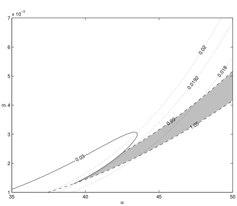
Figure 2: Contours of the inflationary observables $n_{s}$ (dashed) and $\alpha_{s}$ (full) for $N_{\star}=55$. The allowed region is shaded and the dotted contours correspond to different values of $M_{5}$ in units of $M$.

WMAP bounds on the above inflationary observables are, for this class of models (case $\eta>3\epsilon$, class D in Ref. Peiris )

$$0.99<n_{s}<1.28~{},\quad-0.09\leq\alpha_{s}\leq 0.03~{},$$

$$r_{s}\leq 1.10~{}.$$ (26)

These bounds refer to the scale best probed by the CMB observations i.e. $k=0.002$ Mpc^-1; accordingly, we set $N_{k}(k=0.002)=N_{\star}$. On the other hand, bounds on $n_{s}$ from other experiments are less blue, e.g. the combined data sets from BOOMERANG, CBI, DASI, DMR, MAXIMA, TOCO and VSA give comb :

$$0.955<n_{s}<1.05~{}.$$ (27)

In Figure 1, we show contours of the observational bounds on the inflationary observables $n_{s}$, $r_{s}$ and $\alpha_{s}$ in the ($\alpha$, $\beta$) parameter space, for different values of $N_{\star}$; in these plots, we have taken the bounds of Eq. (26) except for the upper bound on $n_{s}$, for which we took the bound of Eq.  (27) instead since such a blue spectrum is not to be expected. We also plotted the $\alpha_{s}=0$ contour, which shows that $\alpha_{s}$ is required to be positive for this model. The shaded area corresponds to the allowed region in parameter space. We would also like to mention that we have checked that it is possible to obtain sufficient inflation with sub-Planckian field values e.g $N=70$ for $\phi_{I}=0.2M_{P}$ and $\alpha,~{}\beta$ within the range specified in Figure 1.

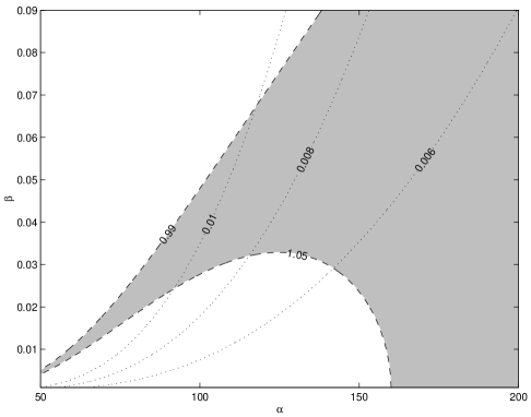
Figure 3: Contours of the inflationary observable $n_{s}$ (dashed) for $N_{\star}=55$ (notice that the range of $\alpha$ and $\beta$ is enlarged as compared with Figure 2). The allowed region is shaded and the dotted contours correspond to different values of $M_{5}$ in units of $M$.

Notice that the contour corresponding to the upper bound on $\alpha_{s}$ is too small to be visible in Figure 1, hence we show it in Figure 2, for $N_{\star}=55$ (similar behavior is obtained for other values of $N_{\star}$), which makes it clear that this bound plays an important role in constraining the parameter space. We obtain lower bounds on $\alpha$ and $\beta$, namely $\alpha>39.23$, pratically independent of $N_{\star}$, whereas the lower bound on $\beta$ ranges from $2.2\times 10^{-3}$ to $1.7\times 10^{-4}$ as $N_{\star}$ ranges from 50 to 75.

In Figures 2 and 3, we have superposed contours of the scale $M_{5}$, as derived from Eqs. (16) and (3), where we have used the COBE normalization i.e. $A_{s}=2\times 10^{-5}$ for $N_{k}=N_{\star}=55$. As the allowed region is quite narrow for low values of $\alpha$, it allows us to find an upper bound on $M_{5}$, $M_{5}\mathrel{\hbox to0.0pt{\lower 4.0pt\hbox{\hskip 1.0pt$\sim$}\hss}\raise 1.0pt\hbox{$<$}}0.0194$ M, which we have checked is almost independent of $N_{\star}$. Combining the above results, we find a lower bound on the scale $V_{0}$, namely $V_{0}^{1/4}\mathrel{\hbox to0.0pt{\lower 4.0pt\hbox{\hskip 1.0pt$\sim$}\hss}\raise 1.0pt\hbox{$<$}}2.1\times 10^{-3}$ M.

Notice that we have chosen to vary $N_{\star}$ since, although a wide variety of assumptions about $N_{\star}$ can be found in the literature, the determination of this quantity requires a model of the entire history of the Universe. However, while from nucleosynthesis onwards this is now well established, at earlier epochs there are considerable uncertanties such as the mechanism ending inflation and details of the reheating process. This issue was recently reviewed in Ref. Liddle2 (see also Ref. Dodelson for similar results), where a model-independent upper bound was derived, namely $N_{\star}<60$; in fact, $N_{\star}=55$ is found to be a reasonable fiducial value with an uncertainty of around 5 around that value; however, the authors stress that there are several ways in which $N_{\star}$ could lie outside that range, in either direction. Moreover, in the braneworld context, one expects $N_{\star}$ to depend on the brane tension. Actually, one expects to obtain larger values of $N_{\star}$ because, in the high-energy regime, the expansion laws corresponding to matter and radiation domination are slower than in the standard cosmology, which implies a greater change in $aH$ relative to the change in $a$, therefore requiring a larger value of $N_{\star}$. This is confirmed by the results of Ref. Wang , where the bound $N_{\star}<75$ is found for brane inspired cosmology.

We have studied the dependence of $n_{s}$ on $k$ to see whether $n_{s}$ can vary from $n_{s}>1$ to $n_{s}<1$ from large to small scales. From the condition $k=aH$, assuming that H is approximatly constant during inflation, we obtain the relation

$$\exp(N_{k})={k_{F}\over k}~{},$$ (28)

where $k_{F}$ is the value of $k$ at the end of inflation. Inserting this relation is Eq. (18), we obtain

$$n_{s}\approx 1+{8\over\alpha}-192{\beta^{2}\over\alpha^{2}}\left({k_{F}\over k}\right)^{8/\alpha}~{},$$ (29)

from which we conclude that, for $\alpha,~{}\beta$ fixed, $n_{s}$ increases with $k$. Hence, it is not possible to obtain the desired behaviour, i.e. $n_{s}$ decreasing from $n_{s}>1$ to $n_{s}<1$ as $k$ increases.

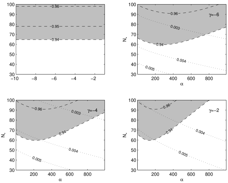
Figure 4: Contours of the inflationary observables $n_{s}$ (dashed) in the ($\alpha,N_{\star}$) plane for the cubic model. The allowed region is shaded and we also show contours corresponding to different values of $M_{5}$ (dotted) in units of $M$. The upper left panel corresponds to the results for this model in the low energy approximation, i.e. without the brane corrections, and the remaining three panels correspond to the high energy approximation for different values of $\gamma$.

III Cubic potential

We shall now consider the case where, due to some cancellation mechanism Adams , the quadratic term is absent and the potential is cubic in $\phi$:

$$V=\Delta^{4}\left[1+\gamma\left(\phi\over M\right)^{3}\right]~{}~{}.$$ (30)

As mentioned before, we shall assume that the first term is dominant. The parameter $\gamma$ is expected to be of order unity and negative Adams ; the model of Ref. Ross corresponds to precisely this case, with $\gamma=-4$.

We start by computing the slow-roll parameters:

$$\epsilon \simeq {18\gamma^{2}\over\alpha}\left({\phi\over M}\right)^{4}~{},$$

$$\eta \simeq {12\gamma\over\alpha}\left({\phi\over M}\right)~{},$$

$$\xi \simeq {72\gamma\over\alpha^{2}}\phi^{2}~{},$$ (31)

where $\alpha\equiv{\Delta^{4}\over\lambda}$.

The value of $\phi$ at the end of inflation can be obtained from Eq. (14); we get, from $|\epsilon|\simeq 1$

$$\phi_{F}\simeq\left({\alpha\over 18\gamma^{2}}\right)^{1/4}M~{},$$ (32)

while, from $|\eta|\simeq 1$, we obtain

$$\phi_{F}\simeq\left({\alpha\over 12|\gamma|}\right)M~{}.$$ (33)

Hence, the prescription to be used depends on the value of $\alpha$. For $\gamma=-4$, we see that the two prescriptions coincide for $\alpha\simeq 26$.

The number of $e$-foldings, $N$, is given by:

$$N={\alpha M\over 6|\gamma|}\left[{1\over\phi_{I}}-{1\over\phi_{F}}\right]~{}~{}.$$ (34)

Therefore, sufficient inflation to solve the cosmological horizon/flatness problems, that is $N>70$, is achieved, for instance for $\gamma=-4$, if $\phi_{I}<7.5\times 10^{-2}M_{P}$.

For $A_{s}$, we obtain, in the high energy regime,

$$A_{s}^{2}\simeq{\alpha^{4}\lambda\over 5400~{}\pi^{2}\gamma^{2}\phi_{k}^{4}}~{}~{},$$ (35)

where $\phi_{k}$ is the value of $\phi$ at horizon-crossing. The scalar spectral index and its running can be readily computed from the slow-roll parameters, Eq. (31), via Eqs.(17) and (19). Notice that the inflationary observables can, of course, be written as a function of $N_{\star}$, as for the quadratic model, using Eq. (34) with $\phi_{I}=\phi_{k}$, but one has to bear in mind that the prescription to use for $\phi_{F}$ depends on $\alpha$.

WMAP bounds on the inflationary observables are, for this class of models (case $\eta<0$, class A in Ref. Peiris )

$$0.94<n_{s}<1.00~{},\quad-0.02\leq\alpha_{s}\leq 0.02~{},$$

$$r_{s}\leq 0.14~{},$$ (36)

again for the scale $k=0.002$ Mpc^-1. In Figure 4, we show contours of the inflationary observable $n_{s}$, $\alpha_{s}$ in the ($\alpha,N_{\star}$) plane. We have checked that neither $\alpha_{s}$ nor $r_{s}$ give further constraints on the parameter space. We also show contours corresponding to different values of $M_{5}$, as given by Eq. (35), again COBE normalized. The upper left panel corresponds to the results for the low energy regime, $V\ll\lambda$, where the brane corrections are negligible, and the remaining three panels correspond to the high energy regime, $V\gg\lambda$, for different values of $\gamma$.

We see that it is the lower bound on $n_{s}$ that most constrains the model and, clearly, $n_{s}=1$ cannot be obtained. It is also clear that, for the model to work, $N_{\star}>65$ is required if brane corrections are not included and $N_{\star}>60$ if those corrections are included; in the latter case, however, this bound increases outside the range $300\mathrel{\hbox to0.0pt{\lower 4.0pt\hbox{\hskip 1.0pt$\sim$}\hss}\raise 1.0pt\hbox{$<$}}\alpha\mathrel{\hbox to0.0pt{\lower 4.0pt\hbox{\hskip 1.0pt$\sim$}\hss}\raise 1.0pt\hbox{$<$}}100$, for $\gamma=-4$ (this range is slightly $\gamma$-dependent, see Figure 4). Moreover, the running parameter is always negative although it can be quite small. Finally, $0.042\ M\mathrel{\hbox to0.0pt{\lower 4.0pt\hbox{\hskip 1.0pt$\sim$}\hss}\raise 1.0pt\hbox{$<$}}M_{5}\mathrel{\hbox to0.0pt{\lower 4.0pt\hbox{\hskip 1.0pt$\sim$}\hss}\raise 1.0pt\hbox{$<$}}0.025\ M$, for $\gamma=-4$ (however, these bounds do not change significantly with $\gamma$, see Figure 4.

Clearly, the spectral index cannot run from $n_{s}>1$ on large scales to $n_{s}<1$ on small scales, since $n_{s}(k)<1$ for this model.

In Ref. Bento2 , a very strict bound on $\alpha$ was derived for this model from the requirement that the reheating temperature is small enough to avoid the gravitino problem. We should like to point out that there was a numerical error in that computation and, in fact, the bound is much weaker and pratically meaningless.

IV Conclusions

We have analysed the implications of WMAP results, in particular the bounds on the inflationary observables, for a class of supergravity inflationary models, Eq. (1) with $n=2,~{}3$. We find that, for the quadratic potential, the main constraints come from the WMAP’s bounds on $n_{s}$ and upper bound on $\alpha_{s}$. We have obtained lower bounds on parameters $\alpha$ and $\beta$, namely $\alpha\mathrel{\hbox to0.0pt{\lower 4.0pt\hbox{\hskip 1.0pt$\sim$}\hss}\raise 1.0pt\hbox{$>$}}39$ (pratically independent of $N_{\star}$) and the lower bound on $\beta$ ranges from $2.2\times 10^{-3}$ to $1.7\times 10^{-4}$ as $N_{\star}$ varies between 50 and 75. We have also found an upper bound on $M_{5}$, $M_{5}\mathrel{\hbox to0.0pt{\lower 4.0pt\hbox{\hskip 1.0pt$\sim$}\hss}\raise 1.0pt\hbox{$<$}}0.0194$ M, pratically independent of $N_{\star}$. Moreover, we conclude that $\alpha_{s}>0$ is required for this model.

For the cubic potential, in the low energy regime i.e. without the brane correction, a relatively high value of $N_{\star}$, $N_{\star}>65$, is required so as to meet WMAP’s lower bound on $n_{s}$. In the high energy regime, when brane corrections are significant, the allowed region in the ($\alpha,N_{\star}$) parameter space changes with $\gamma$ and the main constraints come from WMAP’s lower bound on $n_{s}$. Moreover, we find that $\alpha_{s}<0$ for this model

We have also studied whether it is possible to obtain a running spectral index such that $n_{s}>1$ on large scales and $n_{s}<1$ on small scales and concluded that this is not possible for either model.

- (1) C.L. Bennet et al., Ap. J. Suppl. 148, (2003) 1.
- (2) D.N. Spergel et al., Ap. J. Suppl. 148 (2003) 175.
- (3) V. Barger, H. Lee and D. Marfatia, hep-ph/0302150; U. Seljak, P. McDonald, A. Makarov, Mon. Not. R. Ast. Soc. 342 (2003) L79.
- (4) O. Bertolami, G.G. Ross, Phys. Lett. B183 (1987) 163.
- (5) L. Randall and R. Sundrum, Phys. Rev. Lett. 83 (1999) 4690.
- (6) P. Binétruy, C. Deffayet, U. Ellwanger, D. Langlois, Phys. Lett. B477 (2000) 285; T. Shiromizu, K. Maeda, M. Sasaki, Phys. Rev. D62 (2000) 024012. E.E. Flanagan, S.H. Tye, I. Wasserman, Phys. Rev. D62 (2000) 044039.
- (7) M.C. Bento, O. Bertolami, A.A. Sen, Phys. Rev. D67 (2003) 023504.
- (8) R. Maartens, D. Wands, B.A. Bassett, I.P.C. Heard, Phys. Rev. D62 (2000) 041301.
- (9) M.C. Bento, O. Bertolami, Phys. Rev. D65 (2002) 063513.
- (10) A.R. Liddle, A.J. Smith, Phys. Rev. D68 (2003) 061301.
- (11) D. Langlois, R. Maartens, D. Wands, Phys. Lett. B489 (2000) 259.
- (12) H.V. Peiris et al., Ap. J. Suppl. 148 (2003) 213.
- (13) J.L. Sievers et al., Ap. J. 591 (2003) 599.
- (14) A.R. Liddle, S.M. Leach, Phys. Rev. 68 (2003) 103503.
- (15) S. Dodelson, L. Hui, Phys. Rev. Lett. 91 (2003) 131301.
- (16) B. Wang, E. Abdalla, hep-th/0308145.
- (17) J.A. Adams, G.G. Ross, S. Sarkar, Phys. Lett. B391 (1997) 271.
- (18) G.G. Ross, S. Sarkar, Nucl. Phys. B461 (1995) 597.