CMB Likelihood Functions for Beginners and Experts

Abstract

Although the broad outlines of the appropriate pipeline for cosmological likelihood analysis with CMB data has been known for several years, only recently have we had to contend with the full, large-scale, computationally challenging problem involving both highly-correlated noise and extremely large datasets ($N>1000$). In this talk we concentrate on the beginning and end of this process. First, we discuss estimating the noise covariance from the data itself in a rigorous and unbiased way; this is essentially an iterated minimum-variance mapmaking approach. We also discuss the unbiased determination of cosmological parameters from estimates of the power spectrum or experimental bandpowers.

I Introduction

In principle, CMB anisotropy data analysis is easy: for at least some subset of theories (i.e., inflation) and some subset of CMB experiments, exact likelihood functions can be written down. In these cases, at least, the rest of the problem is implementation: the numerical calculation of the probability distribution of the interesting parameters given the data.

We model a measurement of the CMB as

$$d_{i}=\sum_{p}A_{ip}T_{p}+n_{i}$$ (1)

where $d_{t}$ is the data at time $t_{i}$, $T_{p}$ is the beam-smeared temperature at pixel $p$ (pointed at by unit vector ${\bf\hat{x}}_{p}$), $A_{ip}$ is the pointing operator such that $A_{ip}=1$ when pixel $p$ is observed at time $i$, and $n_{i}$ is the noise at time $i$. The noise is characterised by its distribution, for our purposes assumed to be a Gaussian with covariance $\langle n_{i}n_{i^{\prime}}\rangle=N_{ii^{\prime}}$

Given the data, then, we first wish to solve for the sky temperature $T_{p}$ and its posterior distribution, and then use this map to determine the statistical properties of the CMB sky, such as its power spectrum, $C_{\ell}$ and its distribution, from which we will finally determine the underlying cosmological parameters.

Unfortunately, this implementation is indeed complicated in realistic cases. It is usually assumed that the error distribution for an experiment is somehow handed down to the theorists and data analysts by the experimenters, themselves with a direct link to some higher being who decides these things. Of course this is not actually the case: instead, the error distribution itself must be estimated from the data along with the signal. In some (not necessarily realistic) cases, this is simple. If it were known a priori that the noise were Gaussian and white, then $N_{ii^{\prime}}=\sigma^{2}\delta_{ii^{\prime}}$ and we could use the histogram of observations at a given pixel to estimate the noise variance $\sigma$.

In more realistic cases, the noise in the timestream will be correlated and contaminated by systematic problems and glitches such as cosmic rays, making any simple procedure like this infeasible in practice. In this paper we outline a self-consistent Bayesian (likelihood) method for determining the noise power spectrum along with the CMB map.

Given a map and its statistical distribution (i.e., the error matrix for Gaussian noise), determining the power spectrum (for the case of a Gaussian CMB signal, as well) has been well-studied; problems remain in the implementation of efficient algorithms, but the ideal solution is known.

In this paper, we also address the question of what to do next: how do we go from an estimate of the CMB fluctuation power spectrum, $C_{\ell}$, to the underlying cosmological parameters? Because of the complicated (non-Gaussian) nature of the likelihood function, we will show that simple $\chi^{2}$ techniques will necessarily bias the determination of the parameters, but will derive an ansatz for eliminating this bias.

The plan of this paper is as follows. First, we discuss the CMB Data-Analysis Pipeline from the standpoint of likelihood functions. Then we address the specific problem of simultaneously determining the noise and signal from the timestream. Finally, we address the problem of estimating parameters from the power spectrum.

II Likelihoods for CMB Experiments

As has become customary, we start our analysis with Bayes’ theorem

$$P(\theta|DI)\propto P(\theta|I)P(D|\theta I)$$ (2)

where $\theta$ are the parameters we are trying to determine, $D$ is the data, and $I$ is the “background information” describing the problem. The quantity $P(D|\theta I)$ is thus the likelihood, the probability of the data given a specific set of parameters, $P(\theta|I)$ is the prior probability for the parameters, and the left-hand side of the equation is the posterior probability for the parameters given the data.

As above and throughout, we will take the data, $d_{i}$, as given by a time series of CMB measurements,

$$d_{i}=s_{i}+n_{i}=\sum_{p}A_{ip}T_{p}+n_{i},$$ (3)

where $i$ labels the time, $t=i\delta t$, $s_{i}$ and $n_{i}$ are the experimental noise and sky signal contributions at that time. The signal is in turn given by the operation of a “pointing matrix,” $A_{ip}$ on the sky signal at pixel $p$, $T_{p}$ (i.e., the “map”); we take the latter to be already pixelized and smeared by the experimental beam, so $A$ is a very sparse matrix with a single “1” entry for each time corresponding to the observed pixel. In the future we will often rely on the summation convention and write $\sum_{p}A_{ip}T_{p}=A_{ip}T_{p}$, or occasionally use matrix notation, as in $AT$, etc.

We will assume that the observed noise $n_{i}$ is a realization of a stationary Gaussian process with power spectrum ${\widetilde{N}}(\omega)$. This means that the correlation matrix of the noise is given by

$$\langle n_{i}n_{i^{\prime}}\rangle=N_{ii^{\prime}}=\int{d\omega\over 2\pi}\;{\widetilde{N}}(\omega)e^{-i\omega\delta t(i-i^{\prime})}.$$ (4)

The stationarity of the process requires (or is defined by) $N_{ii^{\prime}}=N(t_{i}-t_{i}^{\prime})$.

Most generally, we will take the parameters to be

• The observed CMB signal on the sky, $T_{p}$;

• The power spectrum of the noise, ${\widetilde{N}}(\omega)$

• (Possibly) any cosmological parameters which describe the distribution of the $T_{p}$ (i.e., the CMB power spectrum, $C_{\ell}$, although we could also use the cosmological paramters such as $H_{0}$ and $\Omega$ directly).

Sometimes, we will assign a prior distribution for the CMB signal such that the cosmological parameters will be irrelevent; other times we will marginalize over the CMB signal itself and determine those parameters.

With these parameters and the data, $d_{i}$, Bayes’ theorem becomes

$$P[T_{p},{\widetilde{N}},C_{\ell}|d_{i},I]\propto P[{\widetilde{N}}|I]\;P(T_{p},C_{\ell}|I)\;P[d_{i}|{\widetilde{N}}(\omega),T_{p},I].$$ (5)

Here, we have used two pieces of information to simplify slightly. First, the noise power spectrum, $N(\omega)$ does not depend at all on the signal, so we can separate out its prior distribution. Second, given the noise power spectrum and the sky signal, the likelihood does not depend upon the cosmological parameters. For the Gaussian noise we assume, the likelihood is simply

$$-2\ln{\cal L} \equiv -2\ln P[d_{i}|{\widetilde{N}},T_{p}]$$ (6)

$$= \ln\left|N_{ii^{\prime}}\right|+\sum_{ii^{\prime}}(d_{i}-s_{i})N^{-1}_{ii^{\prime}}(d_{i^{\prime}}-s_{i^{\prime}})=\sum_{k}\left[\ln{\widetilde{N}}_{k}+|{\tilde{d}}_{k}-{\tilde{s}}_{k}|^{2}/{\widetilde{N}}_{k}\right]$$

(ignoring an additive constant); recall that $s_{i}=\sum_{p}A_{ip}T_{p}$. The second equality uses tildes to denote the discrete Fourier transform at angular frequency $\omega_{k}$ (see appendix and/or below…).

We will now apply these general formulae to various cases.

II.1 Known noise power spectrum

We will start with the simplest case, where we have complete prior knowledge of the noise power spectrum. This is the case that has been previously discussed in the literature, but we emphasize that it is very unrealistic!

We assign a delta-function prior distribution to $N$, transforming it in effect from a parameter to part of the prior knowledge. First, we assume no cosmological information about the distribution of temperatures on the sky: $P(T_{p},C_{\ell}|I)=P(T_{p}|I)P(C_{\ell}|I)$; with this separation the posterior for $C_{\ell}$ is simply the prior—the experiment gives us no new information. We will also assign a uniform prior to $T_{p}$, lacking further information. Now, the posterior distribution for the sky temperature is simply proportional to the likelihood, which can be rewritten by completing the square as

$$P(T_{p}|{\widetilde{N}},d,I)\propto P(d|T_{p},{\widetilde{N}},I)={1\over\left|2\pi C_{Npp^{\prime}}\right|^{1/2}}\exp\left[-{1\over 2}\sum_{pp^{\prime}}\left(T_{p}-{\bar{T}}_{p}\right)C^{-1}_{N,pp^{\prime}}\left(T_{p^{\prime}}-{\bar{T}}_{p^{\prime}}\right)\right]$$ (7)

with the mean (also, the likelihood maximum) given by

$${\bar{T}}=\left(A^{T}N^{-1}A\right)^{-1}A^{T}N^{-1}d$$ (8)

(in matrix notation), and the noise correlation matrix by

$$C_{N}=\left(A^{T}N^{-1}A\right)^{-1}.$$ (9)

Occasionally, the inverse of this correlation matrix is referred to as the weight matrix. As is usual for linear Gaussian models, the mean is just the multidimensional least-squares solution to $d=AT$ with noise correlation $N$. This is just the mapmaking procedure advocated in Refs. wrightprocedure ; tegmaps , cast into the form of a Bayesian parameter-estimation problem.

For the case of known noise, however, this map is more than a just a visual representation of the data. Even if we wish to determine the cosmological parameters, it is an essential quantity. We can write the prior for both the map and the spectrum as

$$P(C_{\ell},T_{p}|I)=P(T_{p}|C_{\ell},I)P(C_{\ell}|I)$$ (10)

using the laws of probability, and so we can see that our rewriting of the likelihood in the form of Eq. 7 remains useful. That is, the full distribution is only a function of the data through the maximum-likelihood map, ${\bar{T}}$—in statistical parlance, ${\bar{T}}$ is a sufficient statistic. Thus for known noise, we can always start by making a map (and calculating its noise matrix, $C_{N}$).

II.1.1 Cosmological CMB priors

Here, we briefly examine the specific form of the signal prior, $P(T_{p}|C_{\ell},I)$, motivated by simple Gaussian models. That is, we take the sky temperature, $T_{p}$, to be an actual realization of a Gaussian CMB sky, with covariance specified by the power spectrum, $C_{\ell}$,

$$\langle T_{p}T_{p^{\prime}}\rangle=C_{T,pp^{\prime}}=\sum_{\ell}\frac{2\ell+1}{4\pi}C_{\ell}B_{\ell}^{2}P_{\ell}\left({\hat{x}}_{p}\cdot{\hat{x}}_{p^{\prime}}\right)$$ (11)

(note that we include beam-smearing by a symmetric beam with spherical harmonic transform $B_{\ell}$ in this definition); ${\hat{x}}_{p}\cdot{\hat{x}}_{p^{\prime}}$ gives the cosine of the angle between the pixels. With this covariance, the prior becomes

$$P(T_{p}|C_{\ell},I)={1\over\left|2\pi C_{Tpp^{\prime}}\right|^{1/2}}\exp\left[-{1\over 2}\sum_{pp^{\prime}}T_{p}C^{-1}_{T,pp^{\prime}}T_{p^{\prime}}\right].$$ (12)

We thus have a posterior distribution for $T_{p}$ and $C_{\ell}$ which is the product of two Gaussians. In the usual cosmological likelihood problem, we don’t care about the actual sky temperature per se, but are concerned with the $C_{\ell}$ (or the parameters upon which the power spectrum depends). Thus, we can marginalize over the $T_{p}$,

$$P(C_{\ell}|d,I) = \int dT_{p}\;P(C_{\ell},T_{p}|d,I)=P(C_{\ell}|I)\int dT_{p}\;P(T_{p}|C_{\ell},I)P(d|T_{p},I)=P(C_{\ell}|I)P({\bar{T}}(d)|C_{\ell}I)$$ (13)

$$= P(C_{\ell}|I){1\over\left|2\pi C_{T}\right|^{1/2}}{1\over\left|2\pi C_{N}\right|^{1/2}}\exp\bigg{[}-{1\over 2}\sum_{pp^{\prime}}\left(T_{p}C^{-1}_{T,pp^{\prime}}T_{p^{\prime}}+\left(T_{p}-{\bar{T}}_{p}\right)C^{-1}_{N,pp^{\prime}}\left(T_{p^{\prime}}-{\bar{T}}_{p^{\prime}}\right)\right)\bigg{]}$$

where we have incuded a prior for the power spectrum itself, so we can write the Gaussian factor as the likelihood for the map given $C_{\ell}$, $P(C_{\ell}|d,I)\propto P(C_{\ell}|I)P({\bar{T}}|C_{\ell})$. The equation defines the effective likelihood for the map (${\bar{T}}$, now considered as the data rather than the timestream itself, $d$), which is easily computed again by completing the square, giving

$$P({\bar{T}}_{p}|C_{\ell}I)={1\over\left|2\pi\left(C_{Tpp^{\prime}}+C_{Npp^{\prime}}\right)\right|^{1/2}}\exp\left[-{1\over 2}\sum_{pp^{\prime}}{\bar{T}}_{p}\left(C_{T}+C_{N}\right)^{-1}_{pp^{\prime}}{\bar{T}}_{p^{\prime}}\right].$$ (14)

This is just the usual CMB likelihood formula: the “observed map,” ${\bar{T}}_{p}$, is just the sum of two quantities (noise and signal) distributed as independent gaussians. Note again that the data only enters through the maximum likelihood map, ${\bar{T}}$, although that calculation is only implicit in this formula. Further, the power spectrum $C_{\ell}$ only enters through the signal correlation matrix, $C_{T}$, and in a very nonlinear way.

We can also play a slightly different game with the likelihood. If we retain the gaussian prior for the CMB temperature but fix the CMB power spectrum, we can estimate the map with this additional prior knowledge. We will again be able to complete the square in the exponential and see that $T_{p}$ is distributed as a gaussian:

$$P(T_{p}|C_{\ell},d,I)={1\over\left|2\pi C_{W}\right|^{1/2}}\exp\left[-{1\over 2}\chi^{2}(T_{p}|C_{\ell},d,I)\right]$$ (15)

with

$$\chi^{2}(T_{p}|C_{\ell},d,I)\equiv\sum_{pp^{\prime}}\ \left({\bar{T}}_{p}-(W{\bar{T}})_{p}\right)C^{-1}_{W,pp^{\prime}}\left({\bar{T}}_{p^{\prime}}-(W{\bar{T}})_{p^{\prime}}\right).$$ (16)

Now, the mean is given by

$$(W{\bar{T}})=C_{T}(C_{T}+C_{N})^{-1}{\bar{T}}$$ (17)

which is just the Wiener Filter! It has correlation matrix given by

$$C_{W}=C_{T}(C_{T}+C_{N})^{-1}C_{T}.$$ (18)

Note that the maximum-likelihood map, ${\bar{T}}$ still appears in these formulae, but it is no longer the maximum of the posterior distribution, now given by the Wiener filter, $W\bar{T}$.

This subsection has shown how many of the usual CMB data calculations can be seen as different uses of the Bayesian formalism:

• the least-squares map (seeing it as a “sufficient statistic”),

• the CMB cosmological-parameter likelihood function, and

• the Wiener filter map of the CMB signal.

The differences depend on what quantity is estimated (the map or the power spectrum) and what prior information is included.

III Simultaneous Estimation of the Noise and Sky Map

We now turn to the (realistic!) case where the noise covariance of the experiment are not known prior to receiving the data. That is, we must use the data itself to estimate the noise properties.

The previous subsection briefly outlined the Bayesian approach to CMB statistics, assuming a known noise power spectrum. Now, we will relax this assumption and approach the more realistic case when we must estimate both the experimental noise and the anisotropy of the CMB. We will take as our model a noise power spectrum of amplitude ${\bar{N}}_{\alpha}$ in bands numbered $\alpha$, with a shape in each band given by a fixed function $P_{k}$ with a width of $n_{\alpha}$ (the number of discrete modes in the band); we will usually take $P_{k}={\rm const}$ so ${\widetilde{N}}$ is piecewise constant. That is,

$${\widetilde{N}}(\omega_{k})={\bar{N}}_{\alpha}P_{k}.$$ (19)

We again assign a constant prior to the sky map, $T_{p}$. As the prior for the noise we will take $P({\bar{N}}_{\alpha})\propto 1/{\bar{N}}_{\alpha}^{\nu}$ With $\nu=1$ and a single band, this is the usual Jeffereys prior advocated for “scale parameters” and the units on ${\bar{N}}_{\alpha}$ are irrelevent.

With this model and priors, the joint likelihood for the noise and the map becomes

$$P(T_{p},{\bar{N}}_{\alpha}|d,I) \propto \prod_{\alpha}{1\over{\bar{N}}_{\alpha}^{\nu+n_{\alpha}/2}}\exp\left[-{1\over 2{\bar{N}}_{\alpha}}\sum_{k\in\alpha}\frac{1}{P_{k}}\left|{\tilde{d}}_{k}-{\widetilde{A}}_{kp}T_{p}\right|^{2}\right]$$ (20)

$$= \prod_{\alpha}{1\over{\bar{N}}_{\alpha}^{\nu+n_{\alpha}/2}}\exp\left[-{1\over 2{\bar{N}}_{\alpha}}\sum_{k\in\alpha}\frac{1}{P_{k}}\left|{\tilde{\varepsilon}}_{k}\right|^{2}\right]$$

where ${k\in\alpha}$ refers to a sum over modes in band $\alpha$. We also define the estimate of the noise as $\varepsilon=d-AT$ for future use.

We can simultaneously solve for the maximum-probability noise and signal. Carrying out the derivatives gives

$${\partial\ln{\cal L}\over\partial T_{p}} = \sum_{\alpha}\left[{1\over{\bar{N}}_{\alpha}}\sum_{k\in\alpha}\frac{1}{P_{k}}\left(d_{k}-A_{kp^{\prime}}T_{p^{\prime}}\right)A_{kp}\right]$$ (21)

$$= (d-AT)^{T}N^{-1}A=\varepsilon^{T}N^{-1}A$$

(switching between indices in Fourier space and matrix notation) and

$${\partial\ln{\cal L}\over\partial{\bar{N}}_{\alpha}}=-{1\over 2}{1\over{\bar{N}}_{\alpha}}\left[(n_{\alpha}+2\nu)-{1\over{\bar{N}}_{\alpha}}\sum_{k\in\alpha}\frac{1}{P_{k}}\left|{\tilde{d}}_{k}-{\widetilde{A}}_{kp^{\prime}}T_{p^{\prime}}\right|^{2}\right]$$ (22)

Setting these to zero and solving, we then find me must simultaneously satisfy

$$T=(A^{T}N^{-1}A)^{-1}A^{T}N^{-1}d$$ (23)

(using matrix notation for simplicity) and

$${\bar{N}}_{\alpha}={1\over n_{\alpha}+2\nu}\sum_{k\in\alpha}\frac{1}{P_{k}}\left|{\tilde{d}}_{k}-{\widetilde{A}}_{kp^{\prime}}T_{p^{\prime}}\right|^{2}={1\over n_{\alpha}+2\nu}\sum_{k\in\alpha}\frac{1}{P_{k}}\left|{\tilde{\varepsilon}}_{k}\right|^{2}.$$ (24)

Equation 23 is just the usual maximum-likelihood map solution; Equation 24 is the average “periodogram” of the noise over the band $\alpha$, with a slight modification for the prior probability, parameterized by $\nu$; for wide bands this is irrelevant. As we will see below, iteration is actually a very efficient way to solve these simulataneously. For future reference, we also write down the derivative with respect to the map at the joint maximum (i.e., substituting Eq. 24 into Eq. 21),

$${\partial\ln{\cal L}\over\partial T_{p}}=\sum_{\alpha}\left[\left(n_{\alpha}+2\nu\right){\sum_{k\in\alpha}{\tilde{\varepsilon}}_{k}{\widetilde{A}}_{kp}/P_{k}\over\sum_{k^{\prime}\in\alpha}\left|{\tilde{\varepsilon}}_{k^{\prime}}\right|^{2}/P_{k^{\prime}}}\right]$$ (25)

If we fix the noise at the joint maximum, then the problem reduces to that of the previous section, a Gaussian likelihood in $T_{p}$ with which the usual tools can be applied. This is not a rigorous approach to the problem, however due to correlation between noise and signal estimation. To get a handle on this, we calculate the curvature of the distribution around this joint maximum, which we define as

$${\cal F}=\left(\begin{array}[]{cc}{\cal G}_{pp^{\prime}}&{\cal G}_{kp}\\ {\cal G}_{pk}&{\cal G}_{kk^{\prime}}\\ \end{array}\right)$$ (26)

where a subscript $\alpha$ or $p$ refers to a derivative with respect to ${\bar{N}}_{\alpha}$ or $T_{p}$, respectively. ${\cal F}$ refers to the full matrix; $\cal G$ to the sub-blocks. Explicitly, the parameter derivatives are

$${\partial^{2}\ln{\cal L}\over\partial T_{p}\partial T_{p^{\prime}}}={\cal G}_{pp^{\prime}}=-\sum_{\alpha}\frac{1}{{\bar{N}}_{\alpha}}\sum_{k\in\alpha}\frac{{\widetilde{A}}_{kp}{\widetilde{A}}_{kp^{\prime}}}{P_{k}}=-A^{T}N^{-1}A$$ (27)

and

$${\partial^{2}\ln{\cal L}\over\partial{\bar{N}}_{\alpha}\partial{\bar{N}}_{\alpha^{\prime}}}={\cal G}_{\alpha\alpha^{\prime}}=-\frac{n_{\alpha}+2\nu}{2{\bar{N}}_{\alpha}^{2}}\delta_{\alpha\alpha^{\prime}}$$ (28)

with the cross-curvature

$${\partial^{2}\ln{\cal L}\over\partial T_{p}\partial{\bar{N}}_{\alpha}}={\cal G}_{p\alpha}=-\frac{1}{{\bar{N}}_{\alpha}^{2}}\sum_{k\in\alpha}\frac{{\tilde{\varepsilon}}_{k}{\widetilde{A}}_{kp}}{P_{k}}$$ (29)

The distribution about the joint maximum is not a Gaussian in the ${\bar{N}}_{\alpha}$ directions, so there is more information available than this. Nonetheless, if we treat the distribution as if it were Gaussian, we can calculate the covariance matrix, given by the inverse of this curvature matrix:

$${\cal F}^{-1}=\left[\begin{array}[]{cc}\left({\cal G}_{pp^{\prime}}-{\cal G}_{p\alpha}{\cal G}^{-1}_{\alpha\alpha^{\prime}}{\cal G}_{\alpha^{\prime}p}\right)^{-1}&\left({\cal G}_{\alpha p}-{\cal G}_{\alpha\alpha^{\prime}}{\cal G}^{-1}_{\alpha^{\prime}p^{\prime}}{\cal G}_{p^{\prime}p}\right)^{-1}\\ \left({\cal G}_{p\alpha}-{\cal G}_{pp^{\prime}}{\cal G}^{-1}_{p^{\prime}\alpha^{\prime}}{\cal G}_{\alpha^{\prime}\alpha}\right)^{-1}&\left({\cal G}_{\alpha\alpha^{\prime}}-{\cal G}_{\alpha p}{\cal G}^{-1}_{pp^{\prime}}{\cal G}_{p^{\prime}\alpha}\right)^{-1}\end{array}\right]$$ (30)

In particular, the effective variance of the map is increased from $C_{N}$ to

$$C^{\rm eff}_{Npp^{\prime}} = (C_{N\ pp^{\prime}}^{-1}-{\cal G}_{p\alpha}{\cal G}^{-1}_{\alpha\alpha^{\prime}}{\cal G}_{\alpha^{\prime}p^{\prime}})^{-1}$$ (31)

$$= \left[\sum_{\alpha}\frac{1}{{\bar{N}}_{\alpha}}\sum_{k\in\alpha}\frac{{\widetilde{A}}_{kp}{\widetilde{A}}_{kp^{\prime}}}{P_{k}}-2\sum_{\alpha}\frac{1}{(n_{\alpha}+2\nu){\bar{N}}^{2}_{\alpha}}\sum_{k\in\alpha}\frac{{\tilde{\varepsilon}}_{k}{\widetilde{A}}_{kp}}{P_{k}}\sum_{k^{\prime}\in\alpha}\frac{{\tilde{\varepsilon}}_{k^{\prime}}{\widetilde{A}}_{k^{\prime}p^{\prime}}}{P_{k^{\prime}}}\right]^{-1}$$

which we have evaluated at the simultaneous peak of the distribution to eliminate ${\bar{N}}_{\alpha}$.

In Ref. FJ99 , we examine this correction to $C_{N}^{-1}$ (the weight matrix) more closely; for sufficiently wide bands, relative to the number of pixels in the map, the correction is negligeable.

III.1 Noise Marginalization

Instead of this joint solution, formally, at least, we know the appropriate procedure: marginalize over the quantity we don’t care about (the noise power spectrum) to obtain the distribution for the quantity we wish to know (the map, $T_{p}$). We can actually carry out this integral in this case:

$$P(T_{p}|d_{i},I)=\int d{\widetilde{N}}_{k}\;P(T_{p},N_{k}|d_{i},I)\propto\prod_{\alpha}\left[\sum_{k\in\alpha}\frac{1}{P_{k}}\left|{\tilde{d}}_{k}-{\widetilde{A}}_{kp}T_{p}\right|^{2}\right]^{-(n_{\alpha}/2+\nu-1)}$$ (32)

(this is just Student’s t distribution in a slightly different form than is usually seen). If we stay in Fourier space, the maximum of this distribution can be calculated to be the solution of

$${\partial\ln P\over\partial T_{p}}=\sum_{\alpha}\left[\left(n_{\alpha}+2\nu-2\right){\sum_{k\in\alpha}\frac{1}{P_{k}}\left(d_{k}-A_{kp^{\prime}}T_{p^{\prime}}\right){\widetilde{A}}_{kp}\over\sum_{k^{\prime}\in\alpha}\frac{1}{P_{k^{\prime}}}\left|d_{k^{\prime}}-{\widetilde{A}}_{k^{\prime}p^{\prime}}T_{p^{\prime}}\right|^{2}}\right]$$ (33)

Note that this is exactly the same form as Eq. 25, the equation for the maximum probability map in the joint estimation case, with the prefactor $(n_{\alpha}+2\nu)$ replaced by $(n_{\alpha}+2\nu-2)$. This is equivalent to changing the exponent of the prior probability from $\nu$ to $\nu-1$: the marginalized maximum for $\nu=1$ (Jefferys prior) is the same as the joint maximum for $\nu=0$ (constant prior). We have also seen that for $n_{\alpha}\gg 1$, the value of $\nu$ is irrelevent, so that these should be nearly equal. (Moreover, the numerical tools to calculate the joint solution, outlined below, can be used in this case, too.) Note also that if $n_{\alpha}+2\nu-2\leq 0$, the equation isn’t solved for any (finite) map. In this case, either our prior information is so unrestrictive or the bands are so narrow that it is impossible to distinguish between noise and signal, and the probability distribution has no maximum when the noise is marginalized.

In principle, any further analysis of the map would have to rely on the full distribution of Eq. 32. In practice, the t-distribution is quite close to a Gaussian [again, for $n_{\alpha}\gg 1$—is this right?] (although the tails are suppressed by a power-law rather than an exponential). It will thus be an excellent approximation to take the distribution to be a Gaussian

$$P(T_{p}|d_{i},I)\approx{1\over\left|2\pi C_{N,pp^{\prime}}^{\rm eff}\right|^{1/2}}\exp\left[-{1\over 2}\sum_{pp^{\prime}}\left(T_{p}-{\bar{T}}_{p}\right)\left(C^{\rm eff}_{N,pp^{\prime}}\right)^{-1}\left(T_{p^{\prime}}-{\bar{T}}_{p^{\prime}}\right)\right]$$ (34)

with noise covariance given by

$$\left(C_{Npp^{\prime}}^{\rm eff}\right)^{-1}=-{\partial^{2}\ln P(T_{p}|d_{i},I)\over\partial T_{p}\partial T_{p^{\prime}}}=\sum_{\alpha}\left[\frac{(n_{\alpha}+2\nu-2)}{\sum_{k\in\alpha}|{\tilde{\varepsilon}}_{k}|^{2}}\sum_{k\in\alpha}\frac{{\widetilde{A}}_{kp}{\widetilde{A}}_{kp^{\prime}}}{P_{k}}-2\frac{(n_{\alpha}+2\nu-2)}{(\sum_{k\in\alpha}|{\tilde{\varepsilon}}_{k}|^{2})^{2}}\sum_{k\in\alpha}\frac{{\tilde{\varepsilon}}_{k}{\widetilde{A}}_{kp}}{P_{k}}\sum_{k^{\prime}\in\alpha}\frac{{\tilde{\varepsilon}}_{k^{\prime}}{\widetilde{A}}_{k^{\prime}p^{\prime}}}{P_{k^{\prime}}}\right]$$ (35)

where ${\bar{T}}$ is the solution to Eq. 33 and the derivatives are taken with respect to the full distribution of Eq. 33). Note that the inverse of $C_{N}^{\rm eff}$ (the weight matrix) is given again by the sum of two terms. The first is just the weight matrix that would be assigned given the maximum probability solution for the noise, Eq. 9 (with the numerically irrelevent change of the prior $\nu\to\nu-1$ as noted above). Again we find a correction term due to the fact that we are only able to estimate this noise power spectrum, where the correction has exactly the same form as in the non-marginalized case (Eq. 31) above with a change of the prefactor.

In Ref. FJ99 , we show how the simultaneous solution for noise and map can be performed iteratively. As we have shown, this is also the solution for the case when the noise is marginalized over.

III.2 Discussion

Happily, the bottom line of this analysis is that the mapmaking phase of CMB data analysis can proceed as has been discussed by other authors in the past. We do recommend two slight additions to the pipeline:

• Iterative map & noise determination

  1. Start by assuming the data stream is all noise.

  2. Calculate the noise power spectrum via FFT.

  3. Inverse FFT, and use this noise matrix for mapmaking

  4. Subtract the estimated signal contribution from the map, and repeat.

• Calculate the correction to the noise matrix (Eq. 35) (and either use the correction or make sure it is negligeable).

We note that it is only necessary to solve for the map itself during the iterative process, but not to invert the inverse noise matrix, $C_{N}^{-}1$. The former can, in principle, be accomplished in far fewer operations than a matrix inverse, so the iterative procedure need not add a great amount of computing time to the process.

However, it is conventional wisdom that an ideal observational strategy has signal to noise of unity. In this regime, the signal to noise in the timestream is very low, and a good aproximation to the estimator of the noise power spectrum is the banded periodogram of the data stream itself. Thus one is able to avoid the time-consuming process of performing multiple iterations.

IV Radical Compression:
From the Power Spectrum to Cosmological Parameters

Above, we discussed how to make a map of the CMB and estimate its noise properties. Elsewhere, the estimation of the CMB anisotropy power spectrum ($C_{\ell}$) from a map and its noise estimate have been described and implemented at least for data sets of moderate size. But the ultimate goal, of course, is to go from the power spectrum to the cosmological parameters. Various groups paramest have calculated how well future experiments are expected to perform; here, we describe what is necessary to begin to achieve such results.

The basic problem is that a plot power spectrum estimates and associated errors do not suffice to describe the likelihood function of the experiment. Usually, we plot ${\cal C}\equiv\ell(\ell+1)C_{\ell}/(2\pi)\pm\sigma_{\ell}$ and are tempted to do a $\chi^{2}$ procedure using those errors and possibly covarinaces between $\ell$ to fit theoretical curves to the estimates. As we have seen above, however, the shape of the likelihood as a function of the $C_{\ell}$ is not Gaussian, implicitly assumed in the use of a $\chi^{2}$ procedure.

One solution is simply to use a full likelihood-minimization procedure on the cosmological parameters given the entire dataset. That is, evaluate Eq. 14 directly for points throughout the cosmological parameter space (over which $C_{\ell}$ and thereby the correlation matrix $C_{T}$ will vary). Since all calculations of the likelihood function to date require $O(N_{\rm pix}^{3})$ operations in general, this is prohibitive for experiments of even moderate size (especially if the likelihood must be searched over something like the 11-dimensional space appropriate for inflation-inspired models).

Instead, we must find efficient ways to approximate the likelihood function based on minimal information. In the rest of this paper, we discuss approximations motivated by our knowledge of the likelihood function. Each requires only knowledge of the likelihood peak and curvature (or variance) as well as a third quantity related to the noise properties of the experiment. Alternately, for already-calculated likelihood functions, each approximation gives a functional form for fitting with a small number of parameters.

IV.1 The solution: approximating the likelihood

IV.1.1 Offset lognormal distribution

We already know enough about the likelihood to see a solution to this problem. For a given multipole $\ell$, there are two distinct regimes of likelihood. Consider a simple all-sky experiment with uniform pixel noise and some symmetric beam. Taking such a map as our data, we write ${\bar{T}}_{p}=T_{p}+n_{p}$ which we transform to spherical harmonics, so the data has contributions from the signal, $a_{\ell m}$, and the noise, $n_{\ell m}$, and the likelihood is

$$-2\ln P({\bar{T}}|{\cal C}_{\ell})=\sum_{\ell}(2\ell+1)\left[\ln\left({\cal C}_{\ell}B_{\ell}^{2}+{\cal N}_{\ell}\right)+{{\widehat{\cal D}}_{\ell}\over{\cal C}_{\ell}B_{\ell}^{2}+{\cal N}_{\ell}}\right]$$ (36)

( up to an irrelevant additive constant; cf. Eq. 14), with ${\cal N}_{\ell}\equiv\ell(\ell+1)N_{\ell}/(2\pi)$, where $N_{\ell}=\langle|n_{\ell m}|^{2}\rangle$ is the noise power spectrum in spherical harmonics, and ${\widehat{\cal D}}_{\ell}\equiv[\ell(\ell+1)/(2\pi)]\ \sum_{m}|a_{\ell m}|^{2}/(2\ell+1)$ is the power spectrum of the full data (noise plus beam-smoothed signal); we have written it as a different symbol from above to emphasize the inclusion of noise and again use script lettering to refer to quantities multiplied by $\ell(\ell+1)/(2\pi)$.

Now, the likelihood is maximized at ${\cal C}_{\ell}=({\widehat{\cal D}}_{\ell}-{\cal N}_{\ell})/B_{\ell}^{2}$ and the curvature about this maximum is given by

$${\cal F}^{({\cal C})}_{\ell\ell^{\prime}}=-{\partial^{2}\ln P({\bar{T}}|{\cal C}_{\ell})\over\partial{\cal C}_{\ell}\partial{\cal C}_{\ell^{\prime}}}={2\ell+1\over 2}\left({\cal C}_{\ell}+{\cal N}_{\ell}/B_{\ell}^{2}\right)^{-2}\delta_{\ell\ell^{\prime}}$$ (37)

so the error (defined by the variance) on a ${\cal C}_{\ell}$ is

$$\delta{\cal C}_{\ell}=\left({\cal C}_{\ell}+{\cal N}_{\ell}/B_{\ell}^{2}\right)/\sqrt{\ell+1/2}.$$ (38)

Note that in this expression there is once again indication of a bias if we assume Gaussianity: upward fluctuations have larger uncertainty than downward fluctuations. But this is not true for $Z_{\ell}$ where $Z_{\ell}$ is defined so that $\delta Z_{\ell}\propto\delta{\cal C}_{\ell}/({\cal C}_{\ell}+{\cal N}_{\ell}/B_{\ell}^{2})$. More precisely, $Z_{\ell}\equiv\ln({\cal C}_{\ell}+{\cal N}_{\ell}/B_{\ell}^{2})$. Since $\delta Z_{\ell}$ is proportional to a constant, our approximation to the likelihood is to take $Z_{\ell}$ as normally distributed. That is, we approximate

$$-2\ln P({\bar{T}}|{\cal C}_{\ell})=\sum_{\ell\ell^{\prime}}Z_{\ell}\left(M^{(Z)}\right)^{-1}_{\ell\ell^{\prime}}Z_{\ell^{\prime}}$$ (39)

(up to a constant) where $M^{(Z)}_{\ell\ell^{\prime}}=({\cal C}_{\ell}+x_{\ell})M^{({\cal C})}_{\ell\ell^{\prime}}({\cal C}_{\ell^{\prime}}+x_{\ell^{\prime}})$ where $M^{({\cal C})}$ is the covariance matrix of the ${\cal C}_{\ell}$, usually taken to be the inverse of the curvature matrix. We refer to Eq. 39 as the offset lognormal distribution of ${\cal C}_{\ell}$. Somewhat more generally we write

$$Z_{\ell}=\ln({\cal C}_{\ell}+x_{\ell})$$ (40)

for some constant $x_{\ell}$, which for the case in hand is $x_{\ell}={\cal N}_{\ell}/B_{\ell}^{2}$.

It is illustrative to derive the quantity $Z_{\ell}$ in a somewhat more abstract fashion. We wish to find a change of variables from ${\cal C}_{\ell}$ to $Z_{\ell}$ such that the curvature matrix is a constant:

$${\partial{\cal F}^{(Z)}_{\ell\ell^{\prime}}\over\partial Z_{\ell}}=0.$$ (41)

That is, we want to find a change of variables such that

$$\left({\cal F}^{(Z)}\right)^{-1}_{LL^{\prime}}=\sum_{\ell\ell^{\prime}}{\partial Z_{L}\over\partial{\cal C}_{\ell}}\left({\cal F}^{({\cal C})}\right)^{-1}_{\ell\ell^{\prime}}{\partial Z_{L^{\prime}}\over\partial{\cal C}_{\ell^{\prime}}}$$ (42)

is not a function of $Z$. We immediately know of one such transformation which would seem to do the trick:

$${\partial Z_{L}\over\partial{\cal C}_{\ell}}={\cal F}_{L\ell}^{1/2}$$ (43)

where the ${1/2}$ indicates a Cholesky decomposition or Hermitian square root. In general, this will be a horrendously overdetermined set of equations, $N^{2}$ equations in $N$ unknowns. However, we can solve this equation in general if we take the curvature matrix to be given everywhere by the diagonal form for the simplified experiment we have been discussing (Eq. 37). In this case, the equations decouple and lose their dependence on the data, becoming (up to a constant factor)

$${dZ_{\ell}\over d{\cal C}_{\ell}}=\left({\cal C}_{\ell}+{\cal N}_{\ell}/B_{\ell}^{2}\right)^{-1}.$$ (44)

The solution to this differential equation is just what we expected,

$$Z_{\ell}=\ln({\cal C}_{\ell}+{\cal N}_{\ell}/B_{\ell}^{2})$$ (45)

with correlation matrix

$$\left({\cal F}^{(Z)}\right)^{-1}_{\ell\ell^{\prime}}={\left({\cal F}^{({\cal C})}\right)^{-1}_{LL^{\prime}}\over\left({\cal C}_{L}+{\cal N}_{L}/B_{L}^{2}\right)\left({\cal C}_{L^{\prime}}+{\cal N}_{L^{\prime}}/B_{L^{\prime}}^{2}\right)}$$ (46)

where $\ell=L$ and $\ell^{\prime}=L^{\prime}$. Please note that we are calculating a constant correlation matrix; the ${\cal C}_{\ell}$ in the denominator of this expression should be taken at the peak of the likelihood (i.e., the estimated quantities).

We emphasize that, even for an all-sky continuously and uniformly sampled experiment (for which Eq. 37 is exact), this Gaussian form, Eq. 39, is only an approximation, since the curvature matrix is given by Eq. 37 only at the peak. Nonetheless we expect it to be a better approximation than a naive Gaussian in ${\cal C}_{\ell}$ (which we note is the limit $x_{\ell}\to\infty$ of the offset lognormal).

We have also considered another ansatz known as the equal variance approximation which we have found sometimes reproduces the shape of the likelihood better than the offset lognormal form above, especially in the case of upper limits on $C_{\ell}$.

IV.2 Noise power

In the above, we have derived the extra quantity needed in this ansatz, $x_{\ell}={\cal N}_{\ell}$, but this was explicitly done only for the unrealistic case of an experiment looking at the whole sky with uniform noise, with a likelihood function Eq. 36. Can we generalize this to more complicated experiments, which have the more complicated likelihood function Eq. 14, with correlation matrices encoding such effects as

• nonuniform noise;

• correlated noise;

• incomplete sky coverage; and/or

• complicated chopping schemes?

Happily, the answer to this question is that we can, and have succesfully applied the results to experiments as diverse as COBE/DMR and Saskatoon.

For a map with noise correlation matrix $C_{N}$, and signal correlation matrix $C_{T}$, we generalize our definition of $x$ to

$${\cal C}_{B}/x_{B}=\sqrt{{\rm Tr}\left(C_{N}^{-1}C_{T,B}C_{N}^{-1}C_{T,B}\right)\over{\rm Tr}\left(C_{T}^{-1}C_{T,B}C_{T}^{-1}C_{T,B}\right)}\simeq\sqrt{{\rm Tr}\left(C_{N}^{-1}C_{T,B}C_{N}^{-1}C_{T,B}\right)\over{\rm Tr}\left(C^{-1}C_{T,B}C^{-1}C_{T,B}\right)}-1$$ (47)

where we use $B$ to label bands of $\ell$ rather than individual multipoles, so that ${\cal C}_{\ell}$ has a fixed shape in each band with amplitude ${\cal C}_{B}$ and $C_{T,B}=\partial C_{T}/\partial{\cal C}_{B}$ is the derivative of the signal correlation matrix with respect to the power in the band. The second expression would be appropriate for a full-sky experiment where the signal and noise separate in the traces; it may be numerically easier to calculate due to zero or negative eigenvalues in $C_{T}$ that often appear due to approximation. Other expressions that may be more appropriate for particular experimental strategies are given in Ref. bjkii .

IV.3 Tests and Results

Because exact likelihoods have been calculated for many different experiments to date, we can check this ansatz in great detail. (In the future, this will probably be impossible because the exact calculation of the likelihood is so expensive that other techniques for finding the maximum will be necessarybcjk99 .)

IV.3.1 COBE/DMR

First, we compare with the likelihood for COBE/DMR at several values of $\ell$. In Fig. 1 we show the actual likelihood for the COBE quadrupole and other multipoles, along with the Gaussian that would be assumed given the curvature matrix calculated from the data. The figures show another way of understanding the bias introduced by assuming Gaussianity: upward deviations from the mean (which is not actually the mean of the non-Gaussian distribution, but the mode) are overly disfavored by the Gaussian distributions while downward ones are overly probable. For example, the standard-CDM value of ${{\cal C}}_{2}=770\mu{\rm K}^{2}$ is only 0.2 times less likely than the most likely value of $150\mu{\rm K}^{2}$ but it seems like a 5-sigma excursion ($4\times 10^{-6}$ times less likely) based on the curvature alone.

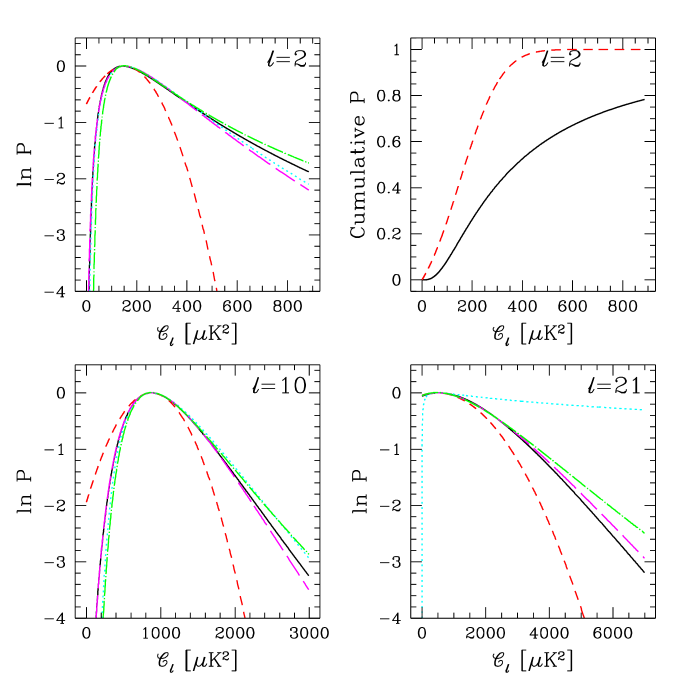
Figure 1: Full and approximate COBE/DMR likelihoods $P(\Delta|{\cal C}_{\ell})$ for various values of $\ell$, as marked. The horizontal axis is ${\cal C}_{\ell}=\ell(\ell+1)C_{\ell}/(2\pi)$. The upper right panel gives the cumulative probability. The solid (black) line is the full likelihood calculated exactly. The short-dashed (red) line is the Gaussian approximation about the peak. The dotted (cyan) line is a Gaussian in $\ln{{\cal C}_{\ell}}$; the dashed (magenta) line is a Gaussian in $\ln{({\cal C}_{\ell}+x_{\ell})}$, as discussed in the text. The dot-dashed (green) line is the equal-variance approximation.

Although it is extremely pronounced in the case of the quadrupole this is a problem that plagues all CMB data: the actual distribution is skewed to allow larger positive excursions than negative. The full likelihood “knows” about this and in fact takes it into account; however, if we compress the data to observed ${\cal C}_{\ell}\pm\sigma_{\ell}$ (or even observed ${\cal C}_{\ell}$ and a correlation matrix $M_{\ell\ell^{\prime}}$) we lose this information about the shape of the likelihood function. Because of its relation to the well-known phenomenon of cosmic variance, we choose to call this problem one of cosmic bias.

We emphasize that cosmic bias can be important even in high-S/N experiments with many pixels. We might expect the central limit theorem to hold in this case and the distributions to become Gaussian. Indeed they do, at least near the peak. However, the central limit theorem does not guarantee that the tails of the distribution will be Gaussian and there is the danger that a few seemingly discrepant points are given considerably more weight than they deserve. Cosmic bias has also been noted in previous work bjki ; uroscopy ; OhSpergelHinshaw .

Putting the problem a bit more formally, we see that even in the limit of infinite signal-to-noise we cannot use a simple $\chi^{2}$ test on ${\cal C}_{\ell}$ estimates; such a test implicitly assumes a Gaussian likelihood. Unlike the distribution discussed here, a Gaussian would have constant curvature ($\delta{\cal C}_{\ell}={\rm constant}$), rather than $\delta{\cal C}_{\ell}\propto{\cal C}_{\ell}$ as illustrated here.

IV.3.2 Saskatoon

We apply this ansatz to the Saskatoon experiment, perhaps the apotheosis of a complicated chopping experiment. The Saskatoon data are reported as complicated chopping patterns (i.e., beam patterns, $H$, above) in a disk of radius about $8^{\circ}$ around the North Celestial Pole. The data were taken over 1993-1995 (although we only use the 1994-1995 data) at an angular resolution of $1.0$–$0.5^{\circ}$ FWHM at approximately 30 GHz and 40 GHz. More details can be found in Refs. nett95 ; woll95 . The combination of the beam size, chopping pattern, and sky coverage mean that Saskatoon is sensitive to the power spectrum over the range $\ell=50$–$350$. The Saskatoon dataset is calibrated by observations of supernova remnant, Cassiopeia–A. Leitch and collaboratorsELthesis have recently measured the flux and find that the remnant is 5% brighter than the previous best determination. We have renormalized the Saskatoon data accordingly.

We calculated ${\cal C}_{\ell}$ for this dataset in bjki . We combine these results with the data’s noise matrix to calculate the appropriate correlation matrixes (in this case, the full curvature matrix) for Saskatoon and hence the appropriate $x_{B}$ (Eq. 47) and thus our approximations to the full likelihood. In Figure 2, we show the full likelihood, the naive Gaussian approximation, and our present offset lognormal and equal-variance forms. Again, both approximations reproduce the features of the likelihood function reasonably well, even into the tails of the distribution, certainly better than the Gaussian approximation. They seem to do considerably better in the higher-$\ell$ bands; even in the lower $\ell$ bands, however, the approximations result in a wider distribution which is preferable to the narrower Gaussian and its resultant strong bias. Moreover, we have found that we are able to reproduce the shape of the true likelihood essentially perfectly down to better than “three sigma” if we simply fit for the $x_{B}$ (but of course this can only be done when we have already calculated the full likelihood—precisely what we are trying to avoid!). For existing likelihood calculations, this method can provide better results without any new calculations (see bjkii for our recommendations for the reporting of CMB bandpower results for extant, ongoing, and future experiments).

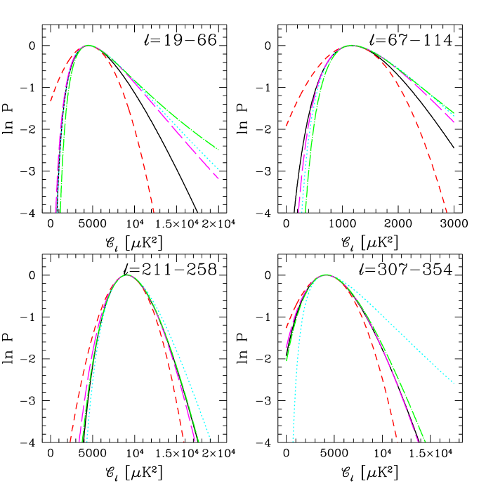
Figure 2: Full and approximate Saskatoon likelihoods. As in Fig. 1. The solid (black) line is the full likelihood calculated exactly. The short-dashed (red) line is the Gaussian approximation about the peak. The dotted (cyan) line is a Gaussian in $\ln{{\cal C}_{\ell}}$; the dashed (magenta) line is a Gaussian in $\ln{({\cal C}_{\ell}+x_{\ell})}$, as discussed in the text. The dot-dashed (green) line is the equal-variance approximation.

We have found that the shape of the power spectrum used with each bin of $\ell$ can have an impact on the likelihood function evaluated using this ansatz. Similarly, a finer binning in $\ell$ will reproduce the full likelihood more accurately. Although the maximum-likelihood amplitude at a fixed shape ($n_{s}$) does not significantly depend on binning or shape, the shape of the likelihood function along the maximum-likelihood ridge changes with finer binning and with the assumed spectral shape.

IV.3.3 COBE/DMR + Saskatoon

As a further example and test of these methods, we can combine the results from Saskatoon and COBE/DMR in order to determine cosmological parameters. For this example, we use the orthogonal linear combinations as described in the previous section. In Figure 3 we show the likelihood contours for standard CDM, varying the scalar slope $n_{s}$ and amplitude $\sigma_{8}$. As before, we see that the naive $\chi^{2}$ procedure is biased toward low amplitudes at fixed shape ($n_{s}$), but that our new approximation recovers the peak quite well. The full likelihood gives a global maximum at $(n_{s},\sigma_{8})=(1.15,1.67)$, and our approximation at $(1.13,1.58)$, while the naive $\chi^{2}$ finds it at $(1.21,1.55)$, outside even the three-sigma contours for the full likelihood. We can also marginalize over either parameter, in which case the full likelihood gives $n_{s}=1.17^{+0.08}_{-0.07}$, $\sigma_{8}=1.68^{+0.26}_{-0.21}$; our ansatz gives $n_{s}=1.14^{+0.07}_{-0.05}$, $\sigma_{8}=1.60\pm 0.15$; and the naive $\chi^{2}$ gives $n_{s}=1.21^{+0.08}_{-0.09}$, $\sigma_{8}=1.55^{+0.18}_{-0.20}$. (Note that even with the naive $\chi^{2}$ we marginalize by explicit integration, since the shape of the likelihood in parameter space is non-Gaussian in all cases.)

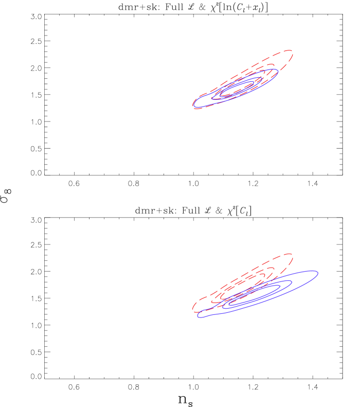
Figure 3: Likelihood contours for COBE/DMR and Saskatoon combined for the cosmological parameters $n_{s}$ and $\sigma_{8}$ (with otherwise standard CDM values) combining likelihoods from COBE/DMR and Saskatoon. Contours are for ratios of the likelihood to its maximum equal to $\exp{-\nu^{2}/2}$ with $\nu=1,2,3$. Upper panel is for the full likelihood (dashed) and its offset lognormal approximation as a Gaussian in $\ln{({\cal C}_{\ell}+x_{\ell})}$ (solid; see text); lower panel shows the full likelihood and its approximation as a Gaussian in ${\cal C}_{\ell}$.

IV.3.4 Parameter Estimation

Above, we have discussed many different approximations to the likelihood ${\cal L}$. Here we discuss finding the parameters that maximize this likelihood (minimize the $\chi^{2}\equiv-2\ln{\cal L}$). We then apply our methods to estimating the power in discrete bins of $\ell$. This application provides another demonstration of the importance of using a better approximation to the likelihood than a Gaussian.

The likelihood functions above depend on ${{\cal C}_{\ell}}$ which may in turn depend on other parameters, $a_{p}$, which are, e.g., the physical parameters of a theory. If we write the parameters as $a_{p}+\delta a_{p}$ we can find the correction, $\delta a_{p}$, that minimizes $\chi^{2}$ by solving

$$\delta a_{p}=-\frac{1}{2}{\cal F}^{-1}_{pp^{\prime}}{\partial\chi^{2}\over\partial a_{p^{\prime}}},$$ (48)

where

$${\cal F}_{pp^{\prime}}\equiv\frac{1}{2}{\partial^{2}\chi^{2}\over\partial a_{p}\partial a_{p^{\prime}}}$$ (49)

is the curvature matrix for the parameters $a_{p}$. If the $\chi^{2}$ were quadratic (i.e., Gaussian ${\cal L}$) then Eq. 48 would be exact. Otherwise, in most cases, near enough to its minimum, $\chi^{2}$ is approximately quadratic and an iterative application of Eq. 48 converges quite rapidly. The covariance matrix for the uncertainty in the parameters is given by $\langle\delta a_{p}\delta a_{p^{\prime}}\rangle={\cal F}^{-1}_{pp^{\prime}}$. This is just an approximation to the Newton-Raphson technique for finding the root of $\partial{\cal L}/\partial a_{p}=0$; a similar techniqe is used in quadratic estimation of ${\cal C}_{\ell}$ tegmark ; bjki ; OhSpergelHinshaw .

As our worked example here, we parameterize the power spectrum by the power in $B=1$ to $11$ bins, ${\cal C}_{B}$. Within each of the bins, we assume ${\cal C}_{\ell}={\cal C}_{B}$ to be independent of $\ell$. We have chosen the offset lognormal approximation. The $\chi^{2}$ completely describes the model:

$$\chi^{2} = \sum_{i,j}\left(Z_{i}^{\rm t}-Z_{i}^{\rm d}\right)M_{ij}^{Z}\left(Z_{j}^{\rm t}-Z_{j}^{\rm d}\right)+\chi^{2}_{\rm cal};$$ (50)

$$\chi^{2}_{\rm cal} \equiv \sum_{\alpha}{(u_{\alpha}-1)^{2}\over\sigma_{\alpha}^{2}};$$ (51)

$$Z_{i}^{\rm d} \equiv \ln(D_{i}+x_{i});$$ (52)

$$Z_{i}^{\rm t} \equiv \ln\left(\sum_{B}u_{\alpha(i)}f_{iB}{\cal C}_{B}+x_{i}\right);$$ (53)

$$M_{ij}^{Z} \equiv M_{ij}\left(D_{i}+x_{i}\right)\left(D_{j}+x_{j}\right)\quad\mbox{no sum};$$ (54)

where $M_{ij}$ is the weight matrix for the band powers $D_{i}$. We have modeled the signal contribution to the data, $D_{i}$, as an average over the power spectrum, $\sum_{B}f_{iB}{\cal C}_{B}$, times a calibration parameter, $u_{\alpha(i)}$. For simplicity, we take the prior probability distribution for this parameter to be normally distributed. Since the datasets have already been calibrated, the mean of this distribution is at $u_{\alpha}=1$. The calibration parameter index, $\alpha$ is a function of $i$ since different power spectrum constraints from the same dataset all share the same calibration uncertainty. We solve simultaneously for the $u_{\alpha}$ and ${\cal C}_{B}$; i.e., together they form the set of parameters, $a_{p}$, in Eq. 48. For those experiments reported as band-powers together with the trace of the window function, $W^{i}_{\ell}$, the filter is taken to be

$$f_{iB}={\sum_{\ell\in B}W^{i}_{\ell}/\ell\over\sum_{\ell}W^{i}_{\ell}/\ell}.$$ (55)

For Saskatoon and COBE/DMR, our $D_{i}$ are themselves estimates of the power in bands. For these cases the above equation applies, but with $W_{\ell}/\ell$ set to a constant within the estimated band and zero outside. The estimated bands have different $\ell$ ranges than the target bands.

Instead of the curvature matrix of Eq. 49 we use an approximation to it that ignores a logarithmic term. Including this term can cause the curvature matrix to be non-positive definite as the iteration proceeds. The approximation has no influence on our determination of the best fit power spectrum, but does affect the error bars. We expect that the effect is quite small.

We now proceed to find the best-fit power spectrum given different assumptions about the value of $x_{i}$, binnings of the power spectrum and editings of the data.

We have determined the $x_{i}$ only for COBE/DMR, Saskatoon, SP89, OVRO7 and SuZIE. To test the sensitivity to the unknown $x_{i}$s we found the minimum-$\chi^{2}$ power spectrum assuming the two extremes of $x_{i}=0$ (corresponding to lognormal) and $x_{i}=\infty$ (corresponding to Gaussian). These two power spectra are shown in Fig. 4. Note that both power spectra were derived using our measured $x_{i}$ values; only the unknown $x_{i}$ values were varied. The variation in the results would be much greater if we let these $x_{i}$ values be at their extremes.

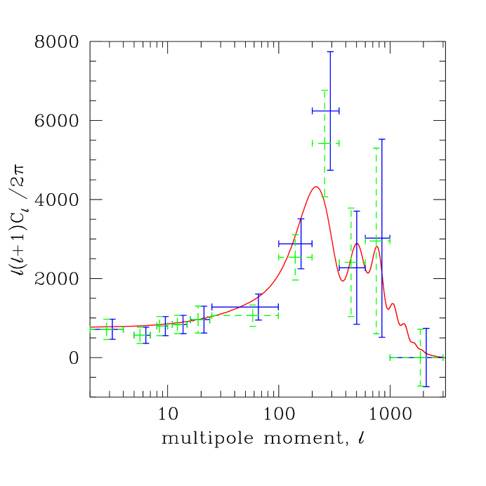
Figure 4: Power spectra that minimize the $\chi^{2}$ in Eq. 50. The solid (dashed) error bars assume $x=0$ ($x=\infty$) for those datasets with no determination of $x$; the two sets have been offset slightly for display purposes. Solid curve is standard CDM.

V Conclusions

In this proceedings, we have discussed the beginning and end of the CMB data-analysis process, and shown how they can be unified in a Bayesian likelihood formalism. We have introduced new techniques and approximations that

• allow simultaneous calculation of the noise properties and underlying sky map.

• approximate the full cosmological likelihood function with minimal information.

Crucially, both of these innovations can be calculated in relatively small or comparable amounts of time to the most computationally-challenging aspects of the problem. Hence, they await the same innovations necessary to perform these calculations in the first place for upcoming megapixel datasetsbcjk99 .

References

- (1) Wright, E.L, astro-ph/9612105.
- (2) Tegmark, M. Astroph. Jour. 455, 1 (1996); Tegmark, M. Phys. Rev. D56, 4514 (1997).
- (3) Ferreira, P.G. & Jaffe, A.H., in preparation (1999).
- (4) See, e.g., Eisenstein, D.J., Hu, W. & Tegmark, M. 1998 astro-ph/9807130; Efstathiou & Bond, 1998, astro-ph/9807103.
- (5) Bond, J.R., Jaffe, A.H. & Knox, L.E., Astrophys. J., submitted (1999).
- (6) Bond, J.R., Crittenden, R.C., Jaffe, A.H. & Knox, L.E., Computers in Science & Engineering, invited review (1999) and references therein.
- (7) Bond, J.R., Jaffe, A.H. & Knox, L.E., Phys. Rev. D57, 2117 (1998) and references therein.
- (8) Seljak, U. 1997, astro-ph/9710269.
- (9) Oh, S.P., Spergel, D.N., and Hinshaw, G. 1998, astro-ph/9805339.
- (10) Netterfield, C.B., Devlin, M.J., Jarosik, N., Page, L., and Wollack, E.J. 1997, Astrophys. J., 474, 47.
- (11) Wollack, E.J., Devlin, M.J., Jarosik, N., Netterfield, C.B., Page, L., and Wilkinson, D. 1997, Astrophys. J., 476, 440.
- (12) Leitch, E. 1998, Caltech PhD. thesis.
- (13) Tegmark, M. 1997, Phys. Rev. D55, 5895; astro-ph/9611174.