PHYSICAL REVIEW D 68, 123521 (2003)
Observational constraints on Chaplygin quartessence: Background results

Abstract

We derive the constraints set by several experiments on the quartessence Chaplygin model (QCM). In this scenario, a single fluid component drives the Universe from a nonrelativistic matter-dominated phase to an accelerated expansion phase behaving, first, like dark matter and in a more recent epoch like dark energy. We consider current data from SNIa experiments, statistics of gravitational lensing, FR IIb radio galaxies, and x-ray gas mass fraction in galaxy clusters. We investigate the constraints from this data set on flat Chaplygin quartessence cosmologies. The observables considered here are dependent essentially on the background geometry, and not on the specific form of the QCM fluctuations. We obtain the confidence region on the two parameters of the model from a combined analysis of all the above tests. We find that the best-fit occurs close to the $\Lambda$CDM limit ($\alpha=0$). The standard Chaplygin quartessence ($\alpha=1$) is also allowed by the data, but only at the $\sim 2\sigma$ level.

I Introduction

Over the past decade, a cosmological model consistent with most astrophysical data available to date has emerged: a flat Universe whose evolution is dominated by a repulsive cosmological term [or dark energy (DE)] and pressureless cold dark matter (CDM). In addition to observational evidence for this model, there are also theoretical motivations for it: for example, inflation theory, which generates a nearly flat space geometry and scale invariant primordial perturbations. Another example regards the nature of the two dark components. Particles predicted by extensions of the standard model of interactions, such as the lightest supersymetric (SUSY) particles susy or the axion axion are, for instance, natural candidates for CDM. On the DE side, a slowly rolling scalar field has been known to produce accelerated expansion since the proposal of inflation. It is thus a well motivated candidate for the cosmological term dynamical . In fact, the simplest and most popular candidate as the driving force for the accelerated expansion is the cosmological constant $\Lambda$. However, its tiny value inferred from present observations creates a major puzzle. If $\Lambda$ is to be considered as the sum of the vacuum energies of all fields, it is hard to understand how they would cancel to one part in $10^{55}$ or 10¹²² (for a review on the cosmological constant and DE, see revde ).

In the standard cosmological model, dark matter and dark energy are necessary to account for two seemingly independent phenomena—clustering of matter and accelerated expansion. As we pointed out, there are some theoretical hints about the nature of these two components, but, in fact, at present, there is no conclusive observational evidence that these phenomena are produced by distinct components (see a first attempt to address this question in Ref. sandvik02 ). Therefore, instead of using a theoretical bias towards dark energy plus CDM, one may choose an alternative point of view and search for phenomenological models that could still be consistent with current observations, motivating theoretical investigations a posteriori. In addition to being potential candidates for the dark sector, these models would allow us to test the robustness of observational predictions regarding the determination of the cosmological model.

From the point of view of simplicity, it would be interesting if instead of two unknown components we could have a single one, accounting for the phenomenology not associated with ordinary matter. In this model, a single component would be responsible for both clustering and accelerated expansion. Such a model is usually referred to as UDM (unifying dark matter energy) or—since there is only one dark component besides baryons, photons, and neutrinos—as quartessence makler03 .

The possibility of a unified description of DE-DM has given rise to rather widespread interest recently. The two major candidates for UDM are the quartessence Chaplygin fluid (QCM) kamenshchik01 ; bilic02 and a quartessence tachyonic field sen02 . Some confrontations of QCM against observational data have been performed. It has been shown that, for a wide range of parameters, this model is consistent with a number of tests of the background metric fabris02 makler03 avelino03 ; colistete03 ; dev03 ; silva03 .

Nevertheless, preliminary analyses of large-scale structure and CMB data favor the $\Lambda$CDM limit of the QCM model sandvik02 ; amendola03 . However, these perturbation analyses need further assumptions beyond the background Chaplygin equation of state. For instance, they assume that there are no viscous stresses in the perturbed fluid. In reis03 it was shown that, if entropy perturbations are allowed, instabilities and oscillations, present in the mass power spectrum in the adiabatic case, may be eliminated and, as a consequence, the parameter space is enlarged.

The main goal of this paper is to set constraints on the Chaplygin quartessence model and check whether it is consistent with present cosmological data. We focus on observables that are dependent essentially on the background geometry. We perform a combined analysis of data, including SNIa experiments, gravitational lensing statistics, FRIIb radio galaxies, and x-ray gas mass fraction in galaxy clusters. Some of these tests were studied previously within the QCM setting. We review these results with a careful treatment and discuss the outcome of a combined analysis of the data.

The paper is organized as follows. In the next section, we discuss the phenomenological motivation for quartessence and present its realization through a fluid with an exotic equation of state, focusing on the QCM. Constraints from SNIa experiments are discussed in Sec. III. In Sec. IV, we discuss the bounds on QCM parameters imposed by the statistics of gravitational lenses. Limits from Fanaroff-Riley type IIb radio galaxies are obtained in Sec. V and from x-ray gas mass fraction in galaxy clusters in Sec. VI. We present a combined analysis of the experiments and our concluding remarks in Sec. VII.

II The Quartessence Chaplygin Model

As discussed in the previous section, the Universe is believed to be dominated by two unknown components, generically denoted by dark energy and dark matter. At the cosmological level, the direct detection of each of these two components involves observations at different scales. Since it is not supposed to cluster at small scales, the effect of dark energy can only be detected over large distances, where the accelerated expansion is observed. On the other hand, the CDM is detected by its local clustering through the motion of visible matter or through the bending of light in gravitational lensing.

Within the standard lore of general relativity and the Friedmann–Lemaître–Robertson–Walker model, for the Universe to undergo acceleration its average density and pressure must obey

$$\left(\rho+3p\right)<0\,,$$ (1)

so that there is an effective gravitational repulsive effect. On the other hand, for the large-scale structures we see to have formed today, the dark matter has to be nonrelativistic, i.e.,

$$\left|p\right|\ll\rho\,.$$ (2)

These two conditions are not in contradiction, since observations in various scales probe different average densities. For example, local motions in clusters of galaxies occur in regions hundreds of times denser than the average density of the Universe. So, if the pressure is negative [as needed from Eq. (1)] and the ratio $\left|p\right|/\rho$ is a decreasing function of the density, the two conditions can be made compatible. In this picture, the quartessence would act as dark energy in very low-density regions and as dark matter in higher-density regions.

A very simple equation of state that has the properties discussed above is the so-called generalized Chaplygin gas kamenshchik01 ,makler01 , bilic02 ,bentoGCG ,

$$p_{\text{Ch}}=-\frac{M^{4(\alpha+1)}}{\rho_{\text{Ch}}^{\alpha}}\,,$$ (3)

where $M$ has the dimension of mass. Consider now the background geometry of the Universe, which can be determined by assuming a homogeneous fluid whose density and pressure are given by the averaged values of the present clumpy matter distribution. In this case, the energy conservation equation

$$\dot{\rho}_{\text{Ch}}=-\left(\rho_{\text{Ch}}+p_{\text{Ch}}\right)3\frac{\dot{a}}{a}$$ (4)

can be easily solved. The energy density of the Chaplygin fluid will be given by

$$\rho_{\text{Ch}}=\rho_{\text{Ch0}}\left[(1-A)\left(\frac{a_{0}}{a}\right)^{3(\alpha+1)}+A\right]^{1/(\alpha+1)}\,,$$ (5)

where $a$ is the scale factor, $a_{0}$ is its present value, $A=(M^{4}/\rho_{ch0})^{(\alpha+1)}$, and the overdot in Eq. (4) denotes the derivative with respect to cosmic time. The equation-of-state parameter and the adiabatic sound velocity, for the Chaplygin component, are given by

$$w_{\text{Ch}}(a)=\frac{p_{\text{Ch}}}{\rho_{\text{Ch}}}=-\frac{Aa^{3(\alpha+1)}}{(1-A)+Aa^{3(\alpha+1)}}$$ (6)

and

$$c_{\text{sCh}}^{2}=\frac{\dot{p}_{\text{Ch}}}{\dot{\rho}_{\text{Ch}}}=-\alpha w_{\text{Ch}}(a)\,.$$ (7)

In principle, the constant $M$ can take any positive value, but we should have $M\sim 10^{-3}$ eV in order to have negative pressure at recent times makler03 . Note that, in QCM, we need $A>1/(3-3\Omega_{b0})$ to have cosmic acceleration starting before the present time ($q_{0}<0$). For instance, for $\Omega_{\text{b}0}=0.04$, the above condition imposes the constraint $A>0.347$. More generically, it is necessary that $A>0$ in order to have a positive cosmological constant at late times. The adiabatic sound speed maximum value (which occurs in the regions where $p_{\text{Ch}}\rightarrow-\rho_{\text{Ch}}$) is given by $\sqrt{\alpha}$. Therefore, the parameter $\alpha$ is restricted to the interval $\alpha\leq 1$. The Chaplygin gas $\alpha=1$ is the extreme case, where the sound velocity can be nearly the speed of light. Another special case is $\alpha=0$, which gives the equation of state $p_{\text{Ch}}=-\rho_{\text{Ch0}}A$ and $\rho_{\text{Ch}}=\rho_{\text{Ch0}}A+\rho_{\text{Ch0}}(1-A)(a_{0}/a)^{3}$, and is, therefore, equivalent to a superposition of CDM and a cosmological constant. Note that, for $\alpha<-1$, we have at early times $w_{\text{Ch}}\sim-1$ and at late times $w_{\text{Ch}}\rightarrow 0$. Thus, since we are interested in the quartessence scenario, where at early times $w_{\text{Ch}}\sim 0$ and at late times $w_{\text{Ch}}\sim-1$, we also impose $\alpha>-1$. For $\rho_{\text{Ch}}$ to be well defined and/or positive at early times, we also impose $A<1$. Therefore in QCM, the parameter $\alpha$ is restricted to the interval $-1<\alpha\leq 1$, and $A$ is restricted to $0<A<1$. We can see that, in fact, in QCM Eq. (5) interpolates between dark matter and dark energy as the average energy density of the Universe changes. That is, when $a/a_{0}\ll 1$, we have $\rho_{\text{Ch}}\propto a^{-3}$ and the fluid behaves as CDM. For late times, $a/a_{0}\gg 1$, and we get $p_{\text{Ch}}=-\rho_{\text{Ch}}=-M^{4}=$ const as in the cosmological constant case.

Equation (3) provides the simplest example of quartessence. It has naturally a single-dimensional constant, since it is given by a power law, and allows us to solve the background energy conservation equation analytically. Besides, it has only two free parameters. However, many other Ansätze for equations of state (EOS) satisfying these criteria can be found.

So far we have introduced the QCM from a purely phenomenological point of view. The EOS in Eq. (3) was chosen as a simple toy model that could allow dark energy/dark matter unification. A completely independent point of view, motivated by brane dynamics, led to the same EOS. Kamenshchik et al. kamenshchik01 proposed EOS in Eq. (3), with $\alpha=1$ (the standard Chaplygin case) as a dark energy candidate. Only after was it realized that such fluid could naturally lead to dark energy/dark matter unification bilic02 . Some possible motivations for this scenario from the field theory point of view are discussed in Refs. kamenshchik01 ; bilic02 ; bentoGCG . The Chaplygin gas appears as an effective fluid associated with the parametrization invariant Nambu-Goto $d$-brane action in a ($d+1,1$) spacetime, and it can also be derived from a Born-Infeld Lagrangian Jackiw99 ; kamenshchik01 . The generalized Chaplygin EOS can be obtained from a complex scalar field Lagrangian with appropriate potential bilic02 ; bentoGCG . The relation between a Chaplygin-like gas and the tachyonic scalar field was investigated in Benaoum .

In the rest of this paper, we will consider only the case of the Chaplygin fluid as quartessence. We will place constraints on the QCM parameters from several cosmological tests which are dependent essentially on the background geometry. We emphasize that the resulting constraints depend on our choice of priors. For example, in Chaplygin quintessence it is commonly assumed that $\Omega_{\text{CDM}}\sim 0.3$, while here we assume $\Omega_{\text{CDM}}=0$. Therefore, the limits on the parameters $\alpha$ and $A$ will be different.

A fundamental quantity related to the observables considered here is the distance-redshift relation, given by

$$r\left(z\right)=\int_{0}^{z}\left[H\left(z^{\prime}\right)\right]^{-1}dz^{\prime}\,,$$ (8)

where $H$ is the Hubble parameter. In the QCM case (neglecting the radiation component), we have

$$H\left(z\right) =H_{0}\left(\left\{\Omega_{b}\left(1+z\right)^{3}\right.\right.$$

$$+\left.\left.\Omega_{\text{Ch}}\left[A+(1-A)\left(1+z\right)^{3\left(1+\alpha\right)}\right]^{1/\left(1+\alpha\right)}\right\}\right)^{1/2}\,,$$ (9)

where $H_{0}$ is the Hubble constant, $z=a_{0}/a-1$ is the redshift, and $\Omega_{\text{Ch}}$, $\Omega_{b}$ are the density parameters of the Chaplygin fluid and baryons, respectively.

Notice that following the idea of unification, we will not include an additional dark matter component. Thus, in Eq. (9) only the baryonic matter scales as $(1+z)^{3}$. Just for $a\ll a_{0}$ does the Chaplygin component scale as CDM. In this case, we have an effective matter density parameter¹

$$\Omega_{m}^{\text{eff}}=\Omega_{\text{Ch}}\left(1-A\right)^{1/\left(1+\alpha\right)}+\Omega_{b}\,.$$ (10)

Notice that, after radiation domination, in this scenario the Universe is always quartessence-dominated, thus avoiding the “why now” problem. However, there is still some fine-tuning to determine whether the average equation of state turns from “matter like” to “energy like” (i.e, when the quartessence pressure begins to play an important role makler03 ).

Because after the decoupling epoch the QCM has negligible pressure, it will cluster as ordinary CDM. In this model, only the unclustered part would lately have appreciable negative pressure.

Since observations of anisotropies in the CMB indicate that the Universe is nearly flat, and since the inflation paradigm predicts a flat geometry, we restrict the following discussions to the zero curvature case, such that $\Omega_{\text{Ch}}+\Omega_{b}=1$.

The baryon density and Hubble parameters can be determined independently of the quartessence model. The observed abundances of light elements together with primordial nucleosynthesis give $\Omega_{b}h^{2}=0.0214\pm 0.0018$ BBN ; DH . The Hubble Space Telescope (HST) key project result is $h=0.72\pm 0.08$ freedman , where $H_{0}:=100h\,$Km/sec/Mpc. These bounds on $\Omega_{b}h^{2}$ and $h$ are in agreement with a fit of purely Wilkinson Microwave Anisotropy Probe (WMAP) and other Cosmic Microwave Background (CMB) data WMAPcospar . Thus, throughout most of this paper we fix the Hubble and the baryon density parameters at $h=0.72$ and $\Omega_{b}=0.041$. With $\Omega_{b}$ and $h$ being determined by independent measurements, in the following sections we will investigate the constraints on the parameters $A$ and $\alpha$ from several experiments, assuming the above-stated priors.

III Type Ia Supernovae Experiments

Supernovae constraints on the Chaplygin models have been analyzed by many authors fabris02 ,makler03 ; avelino03 ; amendola03 , using different priors and simplifications. Here we repeat the analysis presented in makler03 , but we shall not impose any prior on the parameter $A$.

The luminosity distance of a light source is defined in such a way as to generalize to an expanding and curved space the inverse-square law of brightness valid in a static Euclidean space,

$$d_{L}=\left(\frac{L}{4\pi\mathcal{F}}\right)^{1/2}=(1+z)r(z)\,.$$ (11)

In Eq. (11), ${L}$ is the absolute luminosity, $\mathcal{F}$ is the measured flux, and $r(z)$ is given by Eq. (8).

For a source of absolute magnitude $M$, the apparent bolometric magnitude $m(z)$ can be expressed as

$$m(z)=\mathcal{M}+5\log D_{L}\,,$$ (12)

where $D_{L}=D_{L}(z,\alpha,A)$ is the luminosity distance in units of $H_{0}^{-1}$, and

$$\mathcal{M}=M-5\log H_{0}+25$$ (13)

is the “zero point” magnitude (or Hubble intercept magnitude).

We follow the Bayesian approach of Drell, Loredo and Wasserman drell and consider the data of fit C of Perlmutter et al. perlmutter with 16 low-redshift and 38 high-redshift supernovae. In our analysis, we use the following marginal likelihood:

$$\mathcal{L}(\alpha,A)=\frac{s\sqrt{2\pi}}{\Delta\eta}e^{-q/2}\,.$$ (14)

Here

$$q(\alpha,A) =\sum\limits_{i=1}^{16}\frac{(-5\text{log}D_{L}+\nu+m_{\text{B}i}^{\text{corr}})^{2}}{\sigma_{\text{low,}i}^{2}}$$

$$+\sum\limits_{i=1}^{38}\frac{\left(-5\text{log}D_{L}+\nu+m_{\text{B}i}^{\text{eff}}\right)^{2}}{\sigma_{\text{high},i}^{2}}\,,$$ (15)

where

$$\nu(\alpha,A) =s^{2}\,\left(\sum\limits_{i=1}^{16}\frac{5\text{log}D_{L}(z_{i},\alpha,A)-m_{\text{Bi}}^{\text{corr}}}{\sigma_{\text{low,}i}^{2}}\right.$$

$$+\left.\sum\limits_{i=1}^{38}\frac{5\text{log}D_{L}(z_{i},\alpha,A)-m_{\text{B}i}^{\text{eff}}}{\sigma_{\text{high,}i}^{2}}\right)\,,$$ (16)

$$s^{2}=\left(\sum\limits_{i=1}^{16}\frac{1}{\sigma_{\text{low,}i}^{2}}+\sum\limits_{i=1}^{38}\frac{1}{\sigma_{\text{high,}i}^{2}}\right)^{-1}\,,$$ (17)

$$\sigma_{\text{low,}i}^{2}=\sigma_{m_{B,i}^{\text{corr}}}^{2}+\left(\frac{5\;\text{log\thinspace}e}{z_{i}}\sigma_{z_{i}}\right)^{2}$$ (18)

and

$$\sigma_{\text{high,}i}^{2}=\sigma_{m_{B,i}^{\text{eff}}}^{2}+\left(\frac{5\;\text{log\thinspace}e}{z_{i}}\sigma_{z_{i}}\right)^{2}\,.$$ (19)

The quantities $m_{B}^{\text{corr}}$, $m_{B}^{\text{eff}}$, $\sigma_{m_{B}^{\text{corr}}}$, $\sigma_{m_{B}^{\text{eff}}}$ and $\sigma_{z}$ are given in Tables 1 and 2 of Perlmutter et al. perlmutter .

The results of our analysis for the QCM, marginalizing over the intercept, are displayed in Fig. $1$. In this figure, we show $68.3$ and $95.4$ confidence level contours in the $(\alpha,$ $A)$ plane. As we had observed in makler03 , current SNIa data constrain $A$ to the range $0.4\lesssim A\lesssim 0.9$, but do not strongly constrain the parameter $\alpha$ in the considered range.

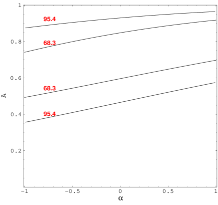
Figure 1: Constant confidence contours ($68.3\%$ and $95.4\%$) in the ($\alpha,A$) plane of the QCM parameters allowed by SNIa data, as described in the text.

IV Gravitational Lensing Statistics

The statistics of gravitational lensing tog is one of the most traditional and widely used methods to constrain cosmological models, especially those with a cosmological constant. Since the publication of the first works on lensing statistics fukugita90 ; fukugita92 ; turn almost 15 years ago, several studies constraining $\Lambda$CDM models krauss ; maoz ; koch93 and some of its variants ratra92 ; bloom ; cooray appeared in the literature. Although not without controversy, before 1998 the general belief was that models with $\Omega_{m0}\sim 1$ and $\Omega_{\Lambda 0}\sim 0$ are preferred by lensing calculations. These results started to be challenged, a few years ago, when the high redshift supernovae observations, in combination with CMB measurements, consistently indicated a nearly flat, low-density, and accelerated Universe. In fact, lensing estimates were not in strong conflict with the supernovae observations. However, it cannot be said also that they were in comfortable agreement. There was room in the parameter space for concordance, mainly if $\Lambda$ is dynamical, but the best-fit regions for each one of the tests were not in good agreement.

With few exceptions, in the past most lensing analyses were based on optically selected quasars. One important concern in lensing investigations with optical sources is extinction in the lensing galaxies. The presence of dust in the lens galaxy could make the quasar images fainter and, as a consequence, difficult to detect. Radio selected surveys are immune to extinction. Besides reducing the total number of multiply imaged systems in an optically selected sample, extinction also affects its angular separation distribution and this is very relevant in lensing analyses. In most studies with optically selected sources, extinction has been neglected. The motivation for this assumption is justified by the fact that early-type galaxies that dominate the lensing statistics are believed to have little dust at the present epoch. However, the possibility that the existence of dust in early-type galaxies at high redshifts ($z>0.5$) could reconcile lensing calculations with models with high $\Lambda$ was suggested 10 years ago by Fukugita and Peebles fukugita93 . Malhotra, Rhoads, and Turner malhotra explored this possibility further and found evidence for it. They estimated a mean extinction of $\Delta m=2\pm 1$ magnitudes. By observing that statistical lensing analyses based on optical and radio observations were not in accordance, Falco et al. fal98 suggested that they can be reconciled if the existence of dust in E/S0 galaxies is considered. However, they estimated that the required mean extinction is considerably lower than that estimated in malhotra . They obtained $\Delta m=0.6\pm 0.4$ mag. In a subsequent work, Falco et al. fal99 concluded that a substantial correction for extinction is necessary in any cosmological estimate using the statistics of lensed quasars. Their directly measured extinction distribution was consistent with statistical estimates from comparison of radio-selected and optically selected lens surveys fal98 .

Another important source of uncertainty in gravitational lensing investigations is the velocity dispersion of early-type galaxies ($\sigma_{\ast}^{(e)}$). The probability of lensing, or the optical depth ($\tau$), depends on the fourth power of $\sigma_{\ast}^{(e)}$ and, hence, is very sensitive to this quantity. In koch96 , Kochanek advocated a high value for the velocity dispersion, namely $\sigma_{\ast}^{(e)}\simeq 225$ Km/sec. Lensing analyses that use relatively high values of $\sigma_{\ast}^{(e)}$ predict low values for $\Lambda$. The reason for this is simple: high $\Lambda$ values imply larger distances and, as a consequence, also larger probability for lensing. In order to have $\tau$ in high-$\Lambda$ models in accordance with observations, one possibility is to “compensate” its increase due to $\Lambda$ by a reduction in $\sigma_{\ast}^{(e)}$. However, this is not so easy. The angular image separation, another observable in lensing statistics, depends on the second power of $\sigma_{\ast}^{(e)}$. Therefore, a too low value of $\sigma_{\ast}^{(e)}$ may not fit the image separation distribution observed in optically selected lens surveys. In fact, the main support for a high $\sigma_{\ast}^{(e)}$ value comes from the angular image separation distribution observed in these surveys. The observed value in the sample used in koch96 is $\left\langle\Delta\theta\right\rangle\simeq 1.6$ $\operatorname{arcsec}$. The sample of radio selected multiply imaged sources used by Falco et al. fal98 in their comparison with the optically selected ones also has a similar high $\left\langle\Delta\theta\right\rangle$.

The situation described above changed considerably with the completion of the Cosmic Lens All Sky Survey (CLASS) sample of radio sources mayers ; browne . Recently, Chae and Chae et al. chae performed a statistical lensing analysis with CLASS data. Under a well-defined selection criterion, they selected a total of 8958 radio sources from the CLASS. From these, a total of 13 systems have multiple images, giving a lensing rate of $\simeq 1/689$. An important difference between the new data and previous ones is that in this sample the mean angular image separation is considerably smaller, $\left\langle\Delta\theta\right\rangle\simeq 1.2$ $\operatorname{arcsec}$. By assuming a singular isothermal ellipsoid as the lens model and a “steep” faint-end slope of early-type galaxies luminosity function ($\alpha^{(e)}=-1$), they determined the velocity dispersion to be $\sigma_{\ast}^{(e)}\simeq 198$ Km/sec. This value is significantly smaller than the best-fit value obtained in koch96 from optically selected surveys. By assuming a flat $\Lambda$CDM model, their likelihood analysis gives ${\Omega_{m0}=0.31}_{-0.14}^{+0.27}$ at the $68\%$ confidence level. They also obtained results without fixing the curvature but fixing the equation of state of the dark energy ($w$) to be $w=-1$, and/or fixing the curvature to be zero and taking $w$ constant but not necessarily equal to $-1$. Their results indicate that, although lensing statistics is less restrictive than the magnitude-redshift test with type Ia supernovae, the two tests are in very good agreement.

Although lensing analyses with radio sources are more reliable, in this work we still use optically selected quasars. We leave for future work the inclusion of radio sources in our analysis.

In the following, we briefly outline our main assumptions for the lensing analysis using highly luminous quasars koch93 ; wm99 . We consider data from the HST Snapshot survey [498 highly luminous quasars (HLQ)], the Crampton survey (43 HLQ), the Yee survey (37 HLQ), the ESO/Liege survey (61 HLQ), the HST GO observations (17 HLQ), the CFA survey (102 HLQ), and the NOT survey (104 HLQ) mao . We consider a total of 862 ($z>1$) highly luminous optical quasars plus five lenses. The lens galaxies are modeled as singular isothermal spheres (SIS), and we consider lensing only by early-type galaxies, since they dominate the lens population. We assume a conserved comoving number density of early-type galaxies peebles02 , $n_{e}=n_{0}(1+z)^{3}$, and a Schechter form sch76 for the early-type galaxy population, $n_{0}=\int_{0}^{\infty}n_{\ast}\left(L/L^{\ast}\right)^{\alpha_{\ast}}\exp\left(-L/L^{\ast}\right)dL/L^{\ast},$ with $n_{\ast}=0.64\pm 0.19\;h^{3}10^{-2}$ $\mbox{Mpc}^{-3}$ and $\alpha_{\ast}=-1.0\pm 0.09$ marzke98 ; chae . We assume that the luminosity satisfies the Faber-Jackson relation fab76 , ${L}/{L^{\ast}}=({\sigma}/{\sigma_{\ast}})^{\gamma}$, with $\gamma=4$ and adopt $\sigma_{\ast}=198$ Km/sec. We emphasize that, even if we consider velocity dispersion of early-type galaxies as low as $\sigma_{\ast}\simeq 190$ Km/sec, extinction has to be considered in order to reconcile the statistical lensing analysis using optically selected sources with those based on CLASS radio-selected sources. Further, if we use $n_{\ast}=0.99\pm 0.05h^{3}10^{-2}$Mpc^-3 and $\alpha_{\ast}=-0.54\pm 0.02$, as obtained by Madgwick et al. madgwick02 , it would be necessary to consider a higher amount of extinction. Previous analyses with optically selected quasars that use high values for $\sigma_{\ast}$ and do not consider extinction are not consistent.

For SIS, the total optical depth ($\tau$) can be expressed analytically, $\tau(z_{S})=F/30\left[d_{A}(1+z_{S})\right]^{3}(cH_{0}^{-1})^{-3},$ where $z_{s}$ is the source redshift, $d_{A}=r(z)/(1+z)$ is its angular diameter distance, and $F=16\pi^{3}n_{\ast}(cH_{0}^{-1})^{3}(\sigma_{\ast}/c)^{4}\Gamma(1+\alpha_{\ast}+4/\gamma)\simeq 0.016$ measures the effectiveness of the lens in producing multiple images tog . We correct the optical depth for the effects of magnification bias and include the selection function due to finite angular resolution and dynamic range koch93 ; koch96 . We assume a mean extinction of $\Delta m=0.6$ mag; this makes the lensing statistics for optically selected quasars consistent with the results of chae .

In Fig. $2$, we show contours of constant likelihood ($95.4\%$ and $68.3\%$) arising from lensing statistics for the quartessence Chaplygin model. It is clear from the figure that lensing statistics weakly constrains these models. Only models with $A\gtrsim 1$ are excluded by the lensing data.

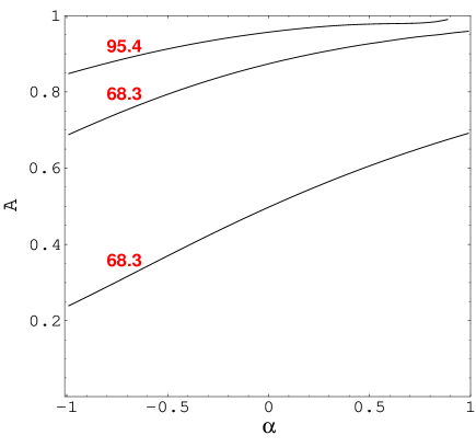
Figure 2: Confidence contours in the ($\alpha,A$) plane from the statistics of optically selected gravitational lenses.

V Fanaroff-Riley Type IIb Radio Galaxies

In addition to gravitational lensing statistics and the SNIa magnitude-redshift test, another useful method to constrain cosmological parameters is the classical angular size-redshift test. In this paper, we shall be concerned with the Fanaroff-Riley type IIb (FR IIb) radio galaxy fanaroff74 version of this test as proposed in daly94 (see also guerra98 ; guerra00 ; daly02 ; podariu03 ). This test consists of a comparison of two independent measures of the average size of the lobe-lobe separation of FR IIb sources, namely the mean size $\left\langle D\right\rangle$ of the full population of radio galaxies at similar redshift and the source average (over its entire life) size $D_{\ast}$, which is determined via a physical model that describes the evolution of the source. The basic idea is that $\left\langle D\right\rangle$ must track the value of $D_{\ast}$, such that the ratio $R_{\ast}=\left\langle D\right\rangle/D_{\ast}$ is independent of redshift. It can be shown that $R_{\ast}\propto r^{(2\beta/3+3/7)}$, where $r$ is the comoving distance, and $\beta$ is a parameter to be determined guerra00 . To determine the confidence region of the parameters of the model, we use the following $\chi^{2}$ function:

$$\chi^{2}=\sum\limits_{i=1}^{20}\frac{\left[R_{\ast},_{i}-c(r,_{i}/r)^{(2\beta/3+3/7)}\right]^{2}}{\sigma_{i}^{2}}\,,$$ (20)

where $r,_{i}=r(z_{i},\Omega_{m0}=0.1,\Omega_{\Lambda 0}=0)$, $\sigma_{i}$ is the combination of the errors in $\left\langle D\right\rangle$ and $D_{\ast}$, and $c$ is a parameter that minimizes the $\chi^{2}$ for fixed values of the cosmological parameters. In our computation, we marginalize over $\beta$ assuming that it is Gaussian distributed such that $\beta=1.75\pm 0.25$ guerra00 .

In Fig. 3, we show contours of constant likelihood ($95.4\%$ and $68.3\%$) arising from the radio galaxies test for the quartessence Chaplygin model. We can see that the FR IIb radio galaxies test also does not strongly constrain the QCM models. Only models with $A\lesssim 0.2$ are excluded by the data at the $95.4\%$ confidence level. However, as we shall see in Sec.VII, when we combine this test with the strong lensing test, we get results similar to those obtained from SNIa.

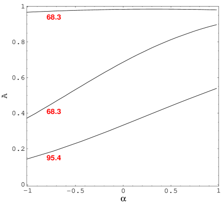
Figure 3: Confidence contours in the ($\alpha,A$) plane allowed by a set of FR IIb radio galaxies.

VI X-ray gas mass fraction in galaxy clusters

In recent years, considerable efforts have been devoted to determining the matter content of clusters of galaxies. Clusters of galaxies are the most recent large-scale structures formed and are also the largest gravitationally bound systems known. Therefore, the determination of their matter content is quite important because cluster properties should approach those of the Universe as a whole. A powerful method based on this idea is to measure the baryon mass fraction $\Omega_{b}/\Omega_{m}$ in rich clusters. By combining this ratio with $\Omega_{b}$ determinations from primordial nucleosynthesis, strong constraints on $\Omega_{m}$ can be placed white . As we shall show, this is especially interesting in quartessence models such as QCM; since the dark sector is unified in these models, any strong constraint on effective dark matter translates directly into a strong constraint on effective dark energy.

Here we use the method and data of Allen, Schmidt, and Fabian allen02 and Allen et al. allen03 . These authors extracted from Chandra observations the x-ray gas mass fraction $f_{\text{gas}}$ of nine massive, dynamically relaxed galaxy clusters, with redshifts in the range $0.08<z<0.47$, and that have converging $f_{\text{gas}}$ within a radius $r_{2500}$ (radius encompassing a region with mean mass density $2500$ times the critical density of the Universe at the cluster redshift).

To determine the confidence region of the parameters of the model, we use the following $\chi^{2}$ function in our computation:

$$\chi^{2}=\sum\limits_{i=1}^{9}\frac{\left[f_{\text{gas}}^{\text{mod}}(z_{i})-f_{\text{gas},i}\right]^{2}}{\sigma_{f_{\text{gas},i}}^{2}}\,,$$ (21)

where $z_{i}$, $f_{\text{gas},i}$, and $\sigma_{f_{\text{gas},i}}$ are, respectively, the redshifts, the SCDM ($h=0.5$) best-fitting values, and the symmetric root-mean-square errors for the nine clusters as given in allen02 and allen03 . In Eq. (21), $f_{\text{gas}}^{\text{mod}}$ is the model function allen02

$$f_{\text{gas}}^{\text{mod}}(z)=\frac{b\Omega_{b}}{(1+0.19\sqrt{h})\Omega_{m}^{\text{eff}}}\left(\frac{h}{0.5}\frac{d_{A}^{\text{EdS}}}{d_{A}^{\alpha,A}}\right)^{3/2}\,.$$ (22)

Here, $d_{A}$ is the angular diameter distance to the cluster, $\Omega_{m}^{\text{eff}}$, given by Eq. (10), is the effective matter density parameter, and $b$ is a bias factor that takes into account the fact that the baryon fraction in clusters could be lower than for the Universe as a whole. In our computations, we marginalize over the bias factor assuming that it is Gaussian-distributed with $b=0.93\pm 0.05$ as suggested by gas-dynamical simulations² bialek01 ; allen03 .

In Fig. $4,$ we show the $68.3\%$ and $95.4\%$ confidence contours on the parameters $\alpha$ and $A$ determined from the Chandra data. The best-fit value, the solid dot in the figure, is located at $\alpha\simeq 0$ and $A\simeq 0.73$ and, as discussed in Sec.II, corresponds to the $\Lambda$CDM limit of QCM. It is clear from the figure that this test is much more restrictive than the others discussed previously.

Figure 4: Constant confidence contours ($68.3\%$ and $95.4\%$) in the ($\alpha,A$) plane determined from the x-ray gas mass fraction in nine galaxy clusters from Chandra data. The best-fit value is indicated by a dot at the center of the contours.

Figure 5: Contours of constant $\Omega_{m}^{\text{eff}}$, corresponding to $\Omega_{m}^{\text{eff}}=0.25$ and $\Omega_{m}^{\text{eff}}=0.35$.

Independent constraints on Chaplygin models from galaxy clusters x-ray data have been presented recently in Ref. cunha03 . In that work, different constraints were obtained; for instance, the contours are quite insensitive to the parameter $A$. In fact, those authors were interested in quintessence Chaplygin, that is, models in which the Chaplygin component behaves only as dark energy, while here we are considering quartessence Chaplygin (no dark matter). Therefore, since Ref. cunha03 started from different priors and did not consider that the Chaplygin component can cluster, it is natural that it reached different conclusions.

It is worth noting that the contours that we have obtained with the Chandra data correspond to constraints on $\Omega_{m}^{\text{eff}}$. To illustrate this, we plot in Fig. $5$ the lines $\Omega_{m}^{\text{eff}}=0.25$ and $\Omega_{m}^{\text{eff}}=0.35$. The similarity of the contours is evident. We remark that constraints on the QCM models similar to those obtained here should be expected from large-scale structure data (assuming entropy perturbations as in reis03 ) that are very sensitive to $\Gamma_{\text{eff}}$, the QCM effective shape parameter of the mass power spectrum sugiyama95 ; beca03 ,

$$\Gamma_{\text{eff}}=\Omega_{m}^{\text{eff}}h\exp\left(-\Omega_{b}-\frac{\sqrt{2h}\Omega_{b}}{\Omega_{m}^{\text{eff}}}\right)\,.$$ (23)

VII Combined analysis and Discussion

Here we summarize our results, presenting a combined analysis of the constraints discussed in the previous sections. In Fig. $6$, we display the allowed region of the parameters $A$ and $\alpha$ from a combination of data from FR IIb galaxies and gravitational lensing. Although $A$ is better constrained than in each one of these experiments separately, it is still not possible to constrain $\alpha$ within our expected interval. Even if we include type Ia supernovae data, as in Fig. $7$, we are not able to constrain this parameter (although the best-fit value is already inside the expected interval); only $A$ can be fairly well constrained with this set. However, the inclusion of cluster x-ray gas mass fraction data, combined with the previous three, as in Fig. $8$, places significant constraints on both $A$ and $\alpha$. These are the tightest constraints on the QCM parameters set to date from the background geometry. The allowed interval of $\alpha$, $-0.5\lesssim\alpha\lesssim 1$, falls within the expected interval discussed in Sec. II. Intriguingly, the best-fit value of $\alpha$ is near the $\Lambda$CDM limit of the model, $\alpha=0$.

It is seen that QCM models with $\alpha\gtrsim-0.5$ are consistent with the observables considered here. Moreover, even the Chaplygin ($\alpha=1$) model—the most theoretically motivated of the QCM family—cannot be ruled out by current observational data.

The aim of this paper was to verify whether the quartessence Chaplygin model is consistent with current data on the background geometry, and to set constraints on the model parameters. As we have discussed in Sec.I, even if the $\Lambda$CDM model is in agreement with the data, it is still interesting to look for alternative models, both from a philosophical point of view and also to test the robustness of the model against observational data, i.e., to sense to which extent we can modify the $\Lambda$CDM paradigm and still be in agreement with the data.

Figure 6: Combined results from the statistics of gravitational lensing and radio galaxies data. We display the $68.3\%$ and $95.4\%$ confidence levels in the ($\alpha,A$) plane.

Figure 7: Combined results from supernovae, gravitational lensing statistics, and radio galaxies data. We display the $68.3\%$ and $95.4\%$ confidence levels in the ($\alpha,A$) plane. The dot is the best-fitting value for the combination of these experiments.

Figure 8: Confidence levels ($68.3\%$ and $95.4\%$) from the combination of all the observables considered in this paper (supernovae, gravitational lensing statistics, radio galaxies, and cluster x-ray gas mass fraction). The best-fit value is located close to the $\Lambda$CDM limit of the model.

We argue that, as a model for dark energy (explanation for accelerated expansion), the Chaplygin gas is not particularly attractive. The most promising feature of it is in the context of quartessence (unification of dark matter and dark energy). Here we have focused on the realization of the quartessence scenario with a fluid whose background equation of state is given by Eq. (3). Rather than favoring a specific model, our results show that alternatives to $\Lambda$CDM are consistent with the data.

We have addressed only observables that probe essentially the distance-redshift relation, and it is clear that one should look for independent tests, such as, for instance, in the large-scale structure of the Universe. In fact, the QCM has a rich behavior regarding the density perturbations. For adiabatic perturbations, the Chaplygin power spectrum has strong oscillations sandvik02 . However, for positive values of $\alpha$, the baryon power spectrum is well behaved beca03 . For some entropy perturbations, the QCM power spectrum itself is well behaved, even for negative values of $\alpha$ reis03 . Therefore, one should investigate further the large-scale distribution of the dark component to better constrain the QCM. In particular, the nonlinear regime of structure formation in QCG models should be more studied. This should shed some light on the issue of the separation into clustered CDM-like and low-density negative pressure regions. The impact on the CMB must also be more studied carturan02 ; bean03 ; bento03 ; amendola03 .

Of course our analysis could be improved in several aspects. For instance, in the lensing analysis, radio sources could be included. Also, we fixed some parameters to their best-fitting values, and they could be marginalized to provide more robust constraints. However, we expect that this will not change qualitatively the results presented here.

The QCM still seems to be a promising model for unifying dark matter and dark energy. More generically, the idea of quartessence has to be explored further, both from the particle physics point of view—to search for a first principles motivation to it—as well as from the empirical side, to constrain quartessence models from observational data.

Acknowledgments

M.M. is partially supported by the FAPERJ. S.Q.O. is partially supported by CNPq. I.W. is partially supported by the Brazilian research agencies CNPq and FAPERJ. We would like to thank Ruth Daly and Erick Guerra for helpful discussions and Steve Allen for useful suggestions and for sending us the gas mass fraction data. We wish also to acknowledge Maurício O. Calvão for useful comments and discussions. M.M. acknowledges the hospitality of the University of Arizona, where part of this work was done.

References

- (1) For a review, see, e.g., K. Griest and M. Kamionkowski, Phys. Rep. 333, 167 (2000).
- (2) For reviews, see, e.g., M. S. Turner, ibid. 197, 67 (1990); G. G. Raffelt, Phys. Rep. 198, 1 (1990).
- (3) B. Ratra and P. J. E. Peebles, Phys. Rev. D 37, 3406 (1988); J. A. Frieman, C. T. Hill, A. Stebbins, and I. Waga, Phys. Rev. Lett. 75, 2077 (1995); P. G. Ferreira and M. Joyce, ibid. 79, 4740 (1997); R. R. Caldwell, R. Dave, P. J. Steinhardt, ibid 80, 1582 (1998).
- (4) P. J. E. Peebles and B. Ratra, Rev. Mod. Phys. 75, 554 (2003). See also V. Sahni and A. Starobinsky, Int. J. Mod. Phys. D 9, 373 (2000); S. M. Carrol, Living Rev. Relativ. 4, 1 (2001).
- (5) H. Sandvik, M. Tegmark, M. Zaldarriaga, and I. Waga, astro-ph/0212114 (v2).
- (6) M. Makler, S. Q. Oliveira, and I. Waga, Phys. Lett. B, 555, 1 (2003).
- (7) A. Kamenshchik, U. Moschella, and V. Pasquier, Phys. Lett. B 511, 265 (2001).
- (8) N. Bilić, G. B. Tupper, and R. D. Viollier, Phys. Lett. B 535, 17 (2002).
- (9) A. Sen, J. High Energy Phys. 04, 48 (2002); G. W. Gibbons, Phys. Lett. B 537, 1 (2002); T. Padmanabhan and T. R. Choudhury, Phys. Rev. D 66, 081301 (2002).
- (10) J. C. Fabris, S. V. B. Goncalves, and P. E. de Souza, astro-ph/0207430 (v1).
- (11) P. P. Avelino, L. M. G. Beça, J. P. M. de Carvalho, C. J. A. P. Martins, and P. Pinto, Phys. Rev. D 67, 023511 (2003).
- (12) A. Dev, J. S. Alcaniz, and D. Jain, Phys. Rev. D 67, 023515 (2003).
- (13) R. Colistete Jr., J. C. Fabris, S. V. B. Goncalves, and P. E. de Souza, astro-ph/0303338 (v1).
- (14) P. T. Silva and O. Bertolami, Astrophys. J. 599, 829 (2003), astro-ph/0303353 (v2).
- (15) L. Amendola, F. Finelli, C. Burigana, and D. Carturan, J. Cosmol. Astropart. Phys. 07, 005 (2003), astro-ph/0304325 (v2).
- (16) R. R. R. Reis, I. Waga, M. O. Calvão, S. E. Jorás,Phys. Rev. D 68, 061302(R) (2003), astro-ph/0306004 (v2).
- (17) M. Makler, Ph.D. thesis, Brazilian Center for Research in Physics, 2001.
- (18) M. C. Bento, O. Bertolami, and A. A. Sen, Phys. Rev. D 66, 043507 (2002).
- (19) R. Jackiw and A. P. Polychronakos, Commun. Math. Phys. 207, 107 (1999); M. Bordemann and J. Hoppe, Phys. Lett. B. 317, 315 (1993).
- (20) H. B. Benaoum, hep-th/0205140 (v1).
- (21) S. Burles, K.M. Nollett, and M.S. Turner, Astrophys. J. Lett. 552, L1 (2001).
- (22) D. Kirkman, D. Tytler, N. Suzuki, J. M. O’Meara, and D. Lubin, Astrophys. J., Suppl. Ser. 149, 1 (2003), astro-ph/0302006 (v1).
- (23) W. Freedman, Astrophys. J. 553, 47 (2001).
- (24) D.N. Spergel et al., Astrophys. J., Suppl. 148, 175 (2003).
- (25) P. S. Drell, T. J. Loredo, and I. Wasserman, Astrophys. J. 530, 593 (2000).
- (26) S. Perlmutter et al., Astrophys. J. 517, 565 (1999).
- (27) E. L. Turner, J. P. Ostriker, and J. R. Gott III, Astrophys. J. 284, 1 (1984).
- (28) M. Fukugita, T. Futamase, and M. Kasai, Mont. Not. R. Astron. Soc. 246, 24 (1990).
- (29) M. Fukugita, T. Futamase, M. Kasai, and E. L. Turner, Astrophys. J. 393, 3 (1992).
- (30) E. L. Turner, Astrophys. J. Lett. 365, L43 (1990).
- (31) L. Krauss and M. White, Astrophys. J. 394, 385 (1992).
- (32) D. Maoz and H. -W. Rix, Astrophys. J. 416, 425 (1993).
- (33) C. S. Kochanek, Astrophys. J. 419, 12 (1993).
- (34) B. Ratra and A. Quillen, Mont. Not. R. Astron. Soc. 259, 738 (1992).
- (35) L. F. Bloomfield and I. Waga, Mont. Not. R. Astron. Soc. 279, 712 (1996).
- (36) A. R. Cooray, Astron. Astrophy., 342, 353 (1999).
- (37) M. Fukugita and P. J. E. Peebles, astro-ph/9305002 (v1).
- (38) S. Malhotra, J. E. Rhoads, and E. L. Turner, Mont. Not. R. Astron. Soc 288, 138 (1997).
- (39) E. E. Falco, C. S. Kochanek, and J. A. Muñoz, Astrophys. J. 494, 47 (1998).
- (40) E. E. Falco et al., Astrophys. J. 523, 617 (1999).
- (41) C. S. Kochanek, Astrophys. J. 466, 47 (1996).
- (42) S. T. Myers et al., Mont. Not. R. Astron. Soc. 341, 1 (2003).
- (43) W. A. Browne et al., Mont. Not. R. Astron. Soc. 341, 13 (2003).
- (44) K. H. Chae et al., Phys. Rev. Lett. 89, 151301 (2002); K. H. Chae, astro-ph/0211244 (v1).
- (45) I. Waga and A. P. M. R. Miceli, Phys. Rev. D 59, 103507 (1999).
- (46) D. Maoz et al., Astrophys. J. 409, 28 (1993); D. Crampton, R. D. McClure, and J. M. Fletcher ibid. J. 392, 23 (1992); H. K. C. Yee, A. V. Filipenko, and D. H. Tang, Astron. J. 105, 7 (1993); A. J. Surdej et al., ibid 105, 2064 (1993); E. E. Falco, in Gravitational Lenses in the Universe, edited by J. Surdej, D. Fraipont-Caro, E. Gosset, S. Refsdal, and M. Remy (University of Liege, Liege, 1993); C. S. Kochanek, E. E. Falco, and R. Shild, Astrophys. J. 452, 109 (1995); A. O. Jaunsen et al., Astron. Astrophys. 300, 323 (1995).
- (47) P. J. E. Peebles, astro-ph/0201015 (v1).
- (48) P. Schechter, Astrophys. J. 203, 297 (1976).
- (49) R. O. Marzke, L. N. da Costa, P. S. Pellegrini, C. N. A. Willmer, and M. J. Geller, Astrophys. J. 503, 617 (1998).
- (50) S. Faber and R. Jackson, Astrophys. J. 204, 668 (1976).
- (51) D. S. Madgwick et al., Mont. Not. R. Astron. Soc. 333, 133 (2002).
- (52) B. L. Fanaroff and J. M. Riley, Mont. Not. R. Astron. Soc. 167, 31 (1974).
- (53) R. A. Daly, Astrophys. J. 426, 38 (1994).
- (54) E. J. Guerra and R. A. Daly, Astrophys. J. 493, 536 (1998).
- (55) E. J. Guerra, R. A. Daly, and L. Wan, Astrophys. J. 544, 659 (2000)
- (56) R. A. Daly and E. J. Guerra, Astrophys. J. 124, 1831 (2002).
- (57) S. Podariu, R. A. Daly, M. P. Mory, and B. Ratra, Astrophys. J. 584, 577 (2003).
- (58) S. D. M. White, J. F. Navarro, A. E. Evrard, and C. Frenk, Nature (London) 366, 429 (1993).
- (59) S. W. Allen, R. W. Schmidt, and A. C. Fabian, Mont. Not. R. Astron. Soc. 334, L11 (2002).
- (60) S. W. Allen, R. W. Schmidt, A. C. Fabian, and H. Ebeling, Mont. Not. R. Astron. Soc. 342, 287 (2003).
- (61) J. J. Bialek, A. E. Evrard, and J. J. Mohr, Astrophys. J. 555, 597 (2001).
- (62) V. R. Eke, J. F. Navarro, and C. S. Frenk, Astrophys. J. 503, 569 (1998).
- (63) S. W. Allen, R. W. Schmidt, and S. L. Bridle, Mon. Not. R. Astron. Soc. 346, 593 (2003), astro-ph/0306386 (v3).
- (64) J. V. Cunha, J. S. Alcaniz, and J. A. S. Lima, astro-ph/0306319 (v1).
- (65) N. Sugiyama, Astrophys. J., Sup. Ser. 100, 281 (1995).
- (66) L. M. G. Beça, P. P. Avelino, J. P. M. de Carvalho, and C. J. A. P. Martins, Phys. Rev. D 67, 101301 (2003).
- (67) D. Carturan and F. Finelli, Phys. Rev. D68, 023515 (2003), astro-ph/0301308 (v1).
- (68) R. Bean and O. Dore, Phys. Rev. D 68, 023515 (2003).
- (69) M. C. Bento, O. Bertolami, and A. A. Sen, Phys. Lett. B 575, 172 (2003), astro-ph/0303538 (v2).