The evolution of galaxy clustering since z=1 from the Calar Alto Deep Imaging Survey (CADIS)

We present results from an investigation of the clustering evolution of field galaxies between a redshift of $z\sim 1$ and the present epoch. The current analysis relies on a sample of $\sim 3600$ galaxies from the Calar Alto Deep Imaging Survey (CADIS). Its multicolor classification and redshift determination is reliable up to $I=23^{\rm mag}$. The redshift distribution extends to $z\sim 1.1$, with formal errors of $\sigma_{z}\simeq 0.02$. Thus the amplitude of the three-dimensional correlation function can be estimated by means of the projected correlation function $w(r_{p})$. The validity of the deprojection was tested on the Las Campanas Redshift Survey (LCRS), which also serves as a “local” measurement. We developed a new method to overcome the influence of redshift errors on $w(r_{p})$. We parametrise the evolution of the clustering strength with redshift by a parameter $q$, the values of which give directly the deviation of the evolution from the global Hubble flow: $\xi(r_{\mathrm{comoving}}=1h^{-1}\mathrm{Mpc})=\xi_{0}(1+z)^{q}$. From a subsample of bright galaxies we find $q=-3.44\pm 0.29$ (for $\Omega_{m}=1$, $\Omega_{\Lambda}=0$), $-2.84\pm 0.30$ (for $\Omega_{m}=0.2$, $\Omega_{\Lambda}=0$), and $q=-2.28\pm 0.31$ (for $\Omega_{m}=0.3$, $\Omega_{\Lambda}=0.7$), that is a significant growth of the clustering strength between $z=1$ and the present epoch. From linear theory of dark matter clustering growth one would only expect $q=-2$ for a flat high-density model. Moreover, we establish that the measured clustering strength depends on galaxy type: galaxies with early type $SED$s (Hubble type: E0 to Sbc) are more strongly clustered at redshifts $z\ga 0.2$ than later types. The evolution of the amplitude of the two-point correlation function for these “old” galaxies is much slower ($q=-0.85\pm 0.82$ for $\Omega_{m}=0.3$, $\Omega_{\Lambda}=0.7$). Since the evolution of the clustering of bright and early type galaxies seems to converge to the same value in the local universe, we conclude that the apparent strong evolution of clustering among all bright galaxies is dominated by the effect that weakly clustered starburst galaxies which are common at high redshifts $z\approx 1.0$ have dimmed considerably since then. Thus the true clustering of massive galaxies is better followed by the early types. This provides both a natural explanation for the seemingly conflicting results of previous studies and accords with the absence of ”faint blue galaxies” in the local universe.

1 Introduction

At the present epoch galaxies are highly clustered and the universe seems to be homogeneous only on the very largest scales. The question of how the structures we see today, and how the galaxies embedded in the dark matter density field have formed and developed, is still one of the most challenging ones in the field of cosmology.

First systematic analyses of the distribution of galaxies and clusters did not occur before galaxy catalogues with large numbers of objects were drawn up – the first analyses of the clustering properties of galaxies were based on the Shane-Wirtanen, the Zwicky catalogue, and the catalogue of Abell clusters, and the results are outlined in a number of fundamental papers by Peebles (and co-workers) (Peebles 1973; Hauser & Peebles 1973; Peebles & Hauser 1974; Peebles 1974; Peebles & Groth 1975; Peebles 1975).

Only a few years later the CfA survey was completed (Davis et al. 1982; Davis & Peebles 1983), and the analysis brought a distribution to light, which was amazingly inhomogeneous – filaments, sheets, walls and large voids emerged, and it became clear that the local universe is in fact far from homogeneous.

The local universe has later been studied using the largest catalogues available today, the Las Campanas Redshift Survey (Shectman et al. 1996), the Sloan Digital Sky Survey (York et al. 2000; Stoughton et al. 2002), and the 2dFGRS (Colless et al. 2001).

It was shown by a number of authors that in the local universe Galaxies are biased tracers of mass, i.e. older galaxies are much more strongly clustered than young, starforming galaxies, bright galaxies are more strongly clustered than faint galaxies (Davis & Geller 1976; Lahav & Saslaw 1992; Santiago & Strauss 1992; Iovino et al. 1993; Hermit et al. 1996; Guzzo et al. 1997; Loveday et al. 1995; Willmer et al. 1998; Norberg et al. 2002; Zehavi et al. 2002a). The exploration of the processes which lead to the different clustering of galaxies of different Hubble types can help us to understand the interaction between the pure structure growth of the dissipationless dark matter component and the development of the baryonic matter into stars and galaxies. In principle, the evolution of the correlation function can also place constraints on the cosmological parameters which determine the geometry and dynamics of our universe. Detailed observations of the evolution of the clustering strength of different galaxy types have to be compared to model predictions (large $N$-body simulations including starformation and feedback, to disentangle dark matter clustering growth and the evolution of the bias. A first attempt was made by Kauffmann et al. (1999a, b), who carried out a semianalytic simulation of galaxy formation and clustering in a $\Lambda$CDM cosmology, in which they analysed the clustering evolution of galaxies with differing luminosity, color, morphology and starformation rate.

For the investigation of structure formation and evolution, measurements of the clustering strength extending to redshifts of $z\ga 1$ are required. Until recently, there have been only few ways to study the large scale structure of the universe at redshifts $z\ga 1$, see for example Le Fèvre et al. (1996), and Carlberg et al. (2000). Not only the shallow depths of most surveys, but also missing redshift information or too small number statistics have limited the possibilities of analysing the data with regard to structure formation. In general, two different types of surveys have to be distinguished – large angle surveys, which are limited to relatively bright apparent magnitudes, and pencil-beam surveys with small, but very deep fields. Furthermore, one can distinguish between surveys that contain only a small number of galaxies, but with very accurate redshift information (deduced from spectroscopy), and surveys that provide huge catalogues of galaxies, but without or with rather limited redshift information. The Calar Alto Deep Imaging Survey (CADIS), see Meisenheimer et al. (2002), is a deep pencil-beam survey, the output of which at present is a catalogue of $\sim 6000$ classified objects to $I\leq 23^{\mathrm{mag}}$. Around $4000$ of these galaxies have reasonably well determined redshifts inferred by means of multicolour methods ($\sigma_{z}\approx 0.02$). This unique data base provides the possibility to investigate the evolution of galaxy clustering from a redshift of $z\approx 1.1$ to the present epoch.

Usually, structure is described in terms of $n$-point correlation functions, the simplest of which is the two-point correlation function. In practice, computing the three-dimensional real-space two-point correlation function requires very accurate distances. Peculiar velocities as well as redshift errors distort the redshift-space relation, and by making the distribution more Poisson-like, increase the noise. Different methods have been developed to overcome these problems. If no redshifts are available at all, it is possible to obtain information about the three dimensional distribution of galaxies by deprojecting the two-dimensional angular correlation function $w(\theta)$. If peculiar velocities are not negligible, or the data suffer from large redshift errors, one can use the deprojection of the projected correlation function (Davis & Peebles 1983) to deduce the clustering strength of the three-dimensional distribution. This method is used to derive the results of the present paper.

This paper is structured as follows: The Calar Alto Deep Imaging Survey and the data used for the analysis are described in Section 2. An introduction into the fundamental principles of three- and two-dimensional correlation functions and the deprojection method used in this paper is given in Section 3. In Section 4 we investigate the evolution of the galaxy clustering from a redshift of $z\sim 1.1$ to today, in Section 5 the results are discussed.

2 The Calar Alto Deep Imaging Survey

The Calar Alto Deep Imaging Survey was established in 1996 as the extragalactic key project of the Max-Planck Institut für Astronomie. It combines a very deep emission line survey carried out with an imaging Fabry-Perot interferometer with a deep multicolour survey using three broad-band optical to NIR filters and up to thirteen medium-band filters when fully completed. The combination of different observing strategies facilitates not only the detection of emission line objects but also the derivation of photometric spectra of all objects in the fields without performing time consuming slit spectroscopy. Details of the survey and its calibration will be given in Meisenheimer et al. (in preparation).

The seven CADIS fields measure $\approx 1/30\leavevmode\nobreak\ \squareforqed\degr$ each and are located at high Galactic latitudes to avoid dust absorption and reddening. In all fields the total flux on the IRAS 100 $\mu$m maps is less than 2 MJy/sr which corresponds to $E_{B-V}<0.07$. Therefore we do not have to apply any colour corrections. As a second selection criterion the fields should not contain any star brighter than $\approx 16^{\mathrm{mag}}$ in the CADIS $R$ band. In fact the brightest star in the four fields under consideration has an $R$ magnitude of $15.42^{\mathrm{mag}}$. Furthermore, the fields are chosen such that there should be at least one field with an altitude of at least $45^{\circ}$ above the horizon of Calar Alto being observable at any time throughout the year. Among the CADIS fields three equatorial fields allow follow-up observations with the VLT.

All observations were performed on Calar Alto, Spain, in the optical wavelength region with the focal reducers CAFOS (Calar Alto Faint Object Spectrograph) at the 2.2 m telescope and MOSCA (Multi Object Spectrograph for Calar Alto) at the 3.5 m telescope. For the NIR observations the Omega Prime camera was used.

In each filter, a set of 5 to 15 individual exposures was taken. The images of one set were then bias subtracted, flatfielded and cosmic corrected, and then coadded to one deep sumframe. This basic data reduction steps were done with the MIDAS software package in combination with the data reduction and photometry package MPIAPHOT (developed by H.-J. Röser and K. Meisenheimer).

2.1 Object detection and classification

Object search is done on the sumframe of each filter using the source extractor software SExtractor (Bertin & Arnouts 1996). The filter-specific object lists are then merged into a master list containing all objects exceeding a minimum $S/N$ ratio in any of the bands. Photometry is done using the program Evaluate, which has been developed by Meisenheimer and Röser (see Meisenheimer & Röser 1986, and Röser & Meisenheimer 1991). Variations in seeing between individual exposures are taken into account, in order to get accurate colours. Because the photometry is performed on individual frames rather than sumframes, realistic estimates of the photometric errors can be derived straightforwardly.

The measured counts are translated into physical fluxes outside the terrestrial atmosphere by using a set of ”tertiary” spectrophotometric standard stars which were established in the CADIS fields, and which are calibrated with secondary standard stars (Oke 1990; Walsh 1995) in photometric nights.

From the physical fluxes, magnitudes and colour indices (an object’s brightness ratio in any two filters, usually given in units of magnitudes) can be calculated. The CADIS magnitude system is described in detail in Wolf et al. (2001c) and Fried et al. (2001).

With a typical seeing of $1\aas@@fstack{\prime\prime}5$ a morphological star-galaxy separation becomes unreliable at $R\ga 21$ where already many galaxies appear compact. Quasars have point-like appearance, and thus can not be distinguished from stars by morphology. Therefore a classification scheme was developed, which is based solely on template spectral energy distributions ($SED$s) (Wolf et al. 2001c, b). The classification algorithm basically compares the observed colours of each object with a colour library of known objects. This colour library is assembled from observed spectra by synthetic photometry performed on an accurate representation of the instrumental characteristics used by CADIS.

The spectral library for galaxies is derived from the mean averaged spectra of Kinney et al. (1996). From these, a grid of 20100 redshifted spectra was formed covering redshifts from $z=0$ to $z=2$ in steps of $\delta z=0.01$ and 100 different intrinsic $SED$s, from old populations to starbursts ($SED=1$ corresponds to an E0 galaxy, whereas $SED=100$ is a starburst galaxy).

Using the minimum variance estimator (for details see Wolf et al. 2001c), each object is assigned a type (star – QSO – galaxy), a redshift (if it is not classified as star), and an $SED$. The formal errors in this process depend on magnitude and type of the object. For the faintest galaxies ($I>22$) they are of the order of $\sigma_{z}=0.02$, and $\sigma_{SED}=2$, respectively.

Note that we do not apply any morphological star/galaxy separation or use other criteria. The classification is purely spectrophotometric.

Details about the performance and reliability of the classification are given in Wolf et al. (2001c), and Wolf et al. (2001b).

Rest-frame luminosities can be estimated directly combining the redshift information and flux measurements in the $16$ filters; we do not apply evolutionary corrections.

Four CADIS fields have been fully analysed so far (for coordinates see Table 1). We identified 4540 galaxies with $I\leq 23$. Out of these, 3626 are located in the redshift range $0.2\leq z\leq 1.07$, where we have analysed their clustering properties. The number of galaxies per field is given in Table 1, together with the number of bright galaxies ($M_{B}<-18+5\log h$).

Table 1: The coordinates of the four fields investigated so far, and the number of galaxies per field, $I\leq 23$ and $0.2\leq z\leq 1.07$, also given is the number of bright galaxies ($M_{B}<-18+5\log h$) in this redshift and apparent magnitude range.

CADIS field	$\alpha_{2000}$	$\delta_{2000}$	$N_{\mathrm{gal}}$	$N_{\mathrm{gal}}^{\mathrm{bright}}$
1 h	$1^{\mathrm{h}}47^{\mathrm{m}}33\aas@@fstack{s}3$	$2^{\circ}19^{\prime}55^{\prime\prime}$	$898$	$740$
9 h	$9^{\mathrm{h}}13^{\mathrm{m}}47\aas@@fstack{s}5$	$46^{\circ}14^{\prime}20^{\prime\prime}$	$916$	$727$
16 h	$16^{\mathrm{h}}24^{\mathrm{m}}32\aas@@fstack{s}3$	$55^{\circ}44^{\prime}32^{\prime\prime}$	$971$	$772$
23 h	$23^{\mathrm{h}}15^{\mathrm{m}}46\aas@@fstack{s}9$	$11^{\circ}27^{\prime}00^{\prime\prime}$	$841$	$660$

The redshift distribution (see Figure 1) has a maximum at $z\approx 0.6$. The large variation between adjacent bins, which is discernably more than expected from Poisson statistics, reflects the large scale structure of the galaxies. With only four fields, the accumulation of galaxies at certain redshifts does not cancel out completely. We analyse the clustering properties of the galaxies between $z=0.2$ and $z=1.07$, where the statistics are large enough and the redshifts are reliable.

Figure 1: Redshift distribution galaxies with $I<23$ in the four CADIS fields. The ”smoothed” redshift distribution can be described by a Gaussian. The dotted lines indicate the redshift range, in which the clustering properties of the galaxies are analysed.

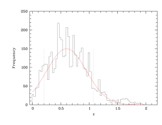
There has never before existed a sample of this depth and size, that includes redshift information. However, the redshift accuracy is not sufficient to calculate the three-dimensional two-point correlation function directly. Nevertheless, as we will demonstrate later, we can use the redshifts for our analysis. First of all it enables us to divide the catalogue into distinct redshift bins and we can analyse the clustering of the galaxies in each of them up to $z\approx 1.1$. Second, we are able to overcome the limitations of the angular correlation function. Instead we can use the projected correlation function, which makes direct use of redshifts, and is less sensitive to redshift errors than the three-dimensional calculation.

We can further divide our sample into different subsamples and investigate the clustering properties of galaxies of different $SED$ types, or different absolute restframe $B$ magnitudes.

3 Three- and two-dimensional correlation functions

The simplest statistic commonly used to describe structure is the two-point correlation function $\xi(r)$. It describes the excess probability of finding pairs of galaxies separated by a distance $r$ over the probability expected in a uniform, random distribution of galaxy locations. Thus, the number of pairs of galaxies ${\mathrm{d}}N_{pair}$ (with one galaxy in the volume element ${\mathrm{d}}V_{1}$ and the other in ${\mathrm{d}}V_{2}$) is given in the form:

$${\mathrm{d}}N_{pair}=N_{0}^{2}[1+\xi(\@vec{r})]{\mathrm{d}}V_{1}\leavevmode\nobreak\ {\mathrm{d}}V_{2}\leavevmode\nobreak\ .$$ (1)

On intermediate scales the correlation function of galaxies is featureless. On very small (kpc) scales a change in the slope is expected (Zehavi et al. 2002b), and on scales $20$ to $30$ Mpc a cutoff in the angular correlation function has been reported (Maddox et al. 1990; Collins et al. 1992; Connolly et al. 2002). However, the smooth, featureless behaviour at the intermediate scales investigated in the present analysis can be parametrised by a power law, as first proposed by Totsuji & Kihara (1969):

$$\xi(r)=\left(\frac{r}{r_{0}}\right)^{-\gamma}\leavevmode\nobreak\ .$$ (2)

The correlation length $r_{0}$ is a measure for the strength of the clustering: the probability of finding a galaxy separated by the distance $r=r_{0}$ from another galaxy is twice as large as for a random distribution of galaxies. Note that the parametrisation by $r_{0}$ is equivalent to determining the correlation amplitude at a specific linear scale.

Since CADIS is a pencil beam survey with a field of view of $11^{\prime}\times 11^{\prime}$, it is of little use to estimate the correlation length $r_{0}$ from the measurement, because it is well outside the measured range of distances. Instead we will deduce the amplitude of $\xi(r)$ at a comoving separation of $r=1h^{-1}$ Mpc.

Throughout this work correlation functions are determined by using the estimator invented by Landy & Szalay (1993):

$$\xi_{\mathrm{LS}} = \frac{\langle DD\rangle-2\langle RD\rangle+\langle RR\rangle}{\langle RR\rangle}\leavevmode\nobreak\ ,$$ (3)

where $\langle DD\rangle$ is the total number of pairs of galaxies in a given radial bin. $\langle RR\rangle$ is the histogram of the distances between pairs of randomly distributed data points that exhibit the same area on the sky, and suffer from the same selection effects as the real data, thus acting as a catalogue window, which is representing the geometrical properties of the survey. $\langle RD\rangle$ is the histogram of the distances between real and random data. Each of the histograms is normalised to the total number of pairs counted.

Random errors of $\xi$ can be calculated from Poisson statistics (Baugh 1996):

$$\sigma_{\mathrm{Poisson}}=\sqrt{\frac{(1+\xi(r))}{[DD]}}\leavevmode\nobreak\ ,$$ (4)

where $[DD]$ is the unnormalised histogram of the number of pairs of real galaxies in logarithmic distance bins. As Baugh (1996) claims, this may underestimate the errors, but they have found that the $2\sigma$ errors computed in this way are comparable to the errors obtained with bootstrap resampling methods (Barrow et al. 1984). As a test we calculated bootstrap errors for one cosmological model and one single redshift bin, and found the same result. Therefore throughout this paper the errors of all correlation functions are calculated following $\sigma_{\xi}=2\sigma_{Poisson}$.

The real space two-point correlation function can only be calculated directly, if redshift information is available with very high precision, and if peculiar velocities are negligible. This is definitely not the case for the multicolour data of CADIS. However, it is possible to derive the parameters by inverting two-dimensional distributions.

3.1 The angular correlation function

The angular correlation function $w(\theta)$ is related to the three dimensional correlation function $\xi(r)$ by Limber’s equation (Limber 1954). Limber’s equation only holds for local samples with $z\ll 1$. For deep samples, which cover a large range of redshifts, the expansion of the universe, curvature effects, and the possible evolution of the clustering have to be included. The redshift-dependent version of Limber’s equation has been derived by Groth & Peebles (1977), and Phillipps et al. (1978). The general distribution of redshifts (${\mathrm{d}}N/{\mathrm{d}}z$) has to be known or calculated from the selection function, which assembles all selection effects due to observation and data reduction.

If $\xi(r)$ is assumed to be a power law (equation (2)), the correlation length $r_{0}$ of the three-dimensional distribution can be calculated.

The disadvantage of this method is that the inversion is highly dependent on the redshift selection function assumed for the survey, which is not a direct observable. Any method which makes direct use of the measured redshifts, like the projected correlation function, gives much more robust results.

3.2 The projected correlation function

If the errors in the redshift measurement are not excessively large, but still too large to facilitate a direct computation, one can use the projected correlation function to derive the correlation length $r_{0}$ and the slope $\gamma$ (Davis & Peebles 1983). It makes use of the redshifts, but is much less sensitive to redshift errors than the three-dimensional correlation function.

For small angles $r^{2}=r_{p}^{2}+\pi^{2}$. The projected correlation function is defined as

$$w(r_{p}) = 2\int_{0}^{\infty}{\xi\left[(r_{p}^{2}+\pi^{2})^{1/2}\right]\leavevmode\nobreak\ {\mathrm{d}}\pi}$$ (5)

$$= 2\int_{r_{p}}^{\infty}{\xi(r)(r^{2}-r_{p}^{2})^{-1/2}r\leavevmode\nobreak\ {\mathrm{d}}r}\leavevmode\nobreak\ ,$$

where $\pi$ is the separation along the line of sight. The projected physical distance $r_{p}$ between galaxies $i$ and $j$ (the distance perpendicular to the line of sight) can – for a given cosmology – be measured very accurately:

$$r_{p}=[d_{A}(i)+d_{A}(j)]\tan(\theta_{ij}/2)\leavevmode\nobreak\ ,$$ (6)

where $d_{A}$ is the angular diameter distance and $\theta_{ij}$ is the apparent separation between galaxy i and galaxy j.

If $\xi(r)=(r/r_{0})^{-\gamma}$, then equation (5) yields

$$w(r_{p})=Cr_{0}^{\gamma}r_{p}^{1-\gamma}\leavevmode\nobreak\ ,$$ (7)

where $C$ is a numerical factor, which depends only on the slope $\gamma$:

$$C=\sqrt{\pi}\frac{\Gamma((\gamma-1)/2)}{\Gamma(\gamma/2)}\leavevmode\nobreak\ .$$ (8)

Thus computing $w(r_{p})$ provides a measurement of the parameters of the three-dimensional correlation function, namely $r_{0}$ and $\gamma$. From the amplitude of $w(r_{p})$ we can deduce the amplitude of the three-dimensional correlation function at $r=1h^{-1}$ Mpc:

With $\xi(r)=(r/r_{0})^{-\gamma}$

$$\xi(r=1h^{-1}\mathrm{Mpc})=r_{0}^{\gamma}$$ (9)

$$w(r_{p}) = Cr_{p}^{1-\gamma}r_{0}^{\gamma}$$ (10)

$$= Cr_{p}^{1-\gamma}\xi(r=1h^{-1}\mathrm{Mpc})$$

The expressions (5) to (10) refer to physical distances as would be measured by an observer at the epoch under consideration. To facilitate a direct comparison of the possible changes with respect to the global Hubble flow, we compute the amplitude for a comoving distance $r_{\rm com}=1h^{-1}$ Mpc. With

$$\xi(r_{\rm com}=1h^{-1}\mathrm{Mpc}) = (r_{0}(1+z))^{\gamma}\leavevmode\nobreak\ ,$$ (11)

which we will call $\xi_{1\mathrm{Mpc}}$ in the following, we find

$$\Rightarrow\xi_{1\mathrm{Mpc}}=\frac{w(r_{p})(1+z)^{\gamma}}{Cr_{p}^{1-\gamma}}\leavevmode\nobreak\ ,$$ (12)

with the numerical factor C from equation (8).
The errors are calculated following Gaussian error propagation:

$$\sigma_{\xi_{1\mathrm{Mpc}}}=\left[\left(\frac{\partial\xi_{1\mathrm{Mpc}}}{\partial w(r_{p})}\sigma_{w(r_{p})}\right)^{2}\!\!\!+\!\!\!\left(\frac{\partial\xi_{1\mathrm{Mpc}}}{\partial\gamma}\sigma_{\gamma}\right)^{2}\right]^{\frac{1}{2}}$$ (13)

In our case the error of $\gamma$ is negligible, as explained in the following section. The first term completely dominates the error of $\xi_{1\mathrm{Mpc}}$, thus the approximation $\sigma_{\log\xi_{1\mathrm{Mpc}}}=\sigma_{\log A}$ is valid within a fraction of the statistical error.

The mean galaxy density is determined from the observed galaxy counts in each field, which does not necessarily represent the the true density (Groth & Peebles 1977). The estimator will be on average biased low with respect to the true correlation by a constant amount

$${\cal I}\approx\frac{1}{S^{2}}\int{w_{\rm true}(r_{p})\mathrm{d}^{2}S_{1}\mathrm{d}^{2}S_{2}}\leavevmode\nobreak\ ,$$ (14)

where $w_{true}(r_{p})$ is the true projected correlation function and $S$ is the physical area corresponding to the solid angle of the field at the redshift under consideration. If the true correlation function is given by equation (10), the measurement yields

$$w_{m}(r_{p}) = Cr_{0}^{\gamma}r_{p}^{1-\gamma}-{\cal I}$$ (15)

$$= Cr_{0}^{\gamma}\left[r_{p}^{1-\gamma}-{\cal I}/(Cr_{0}^{\gamma})\right]\leavevmode\nobreak\ .$$ (16)

The true amplitude $Cr_{0}^{\gamma}$ is not known, but ${\cal I}/(Cr_{0}^{\gamma})$ can be estimated by performing a Monte Carlo integration (where we use the mean of the pair counts $\langle RR\rangle$ at a projected distance $r_{p}$ of the four fields):

$$\frac{{\cal I}}{Cr_{0}^{\gamma}}=\frac{\sum{\left[\langle RR\rangle\cdot r_{p}^{1-\gamma}\right]}}{\sum{\langle RR\rangle}}\leavevmode\nobreak\ .$$ (17)

The true value of $Cr_{0}^{\gamma}$ can be estimated by fitting equation (16) to the data, taking the value of ${\cal I}/(Cr_{0}^{\gamma})$ from equation (17). This value, multiplied by the fitted amplitude $Cr_{0}^{\gamma}$, yields the integral constraint ${\cal I}$. This constant will then be added to the measured amplitude $A$, and from the so corrected amplitude the value of $\xi_{1\mathrm{Mpc}}$ will be inferred by means of equation (12).

3.2.1 Estimation of the projected correlation function

Following Davis & Peebles (1983) one can calculate the projected correlation function from

$$w(r_{p})=\int_{-\delta\pi}^{+\delta\pi}{\xi(r_{p},\pi)\leavevmode\nobreak\ {\mathrm{d}}\pi}\leavevmode\nobreak\ .$$ (18)

Since the three-dimensional two-point correlation function has the form of a power law, it converges rapidly to zero with increasing pair separation. Therefore the integration limits do not have to be $\pm\infty$, they only have to be large enough to include all correlated pairs. Since the direct observable is the redshift $z$ instead of the physical separation along the line of sight, we make use of a coordinate transformation (Le Fèvre et al. 1996):

$$w(r_{p})=\int_{-\delta z}^{+\delta z}{\xi(r_{p},\pi)\frac{{\mathrm{d}}\pi}{{\mathrm{d}}z}\leavevmode\nobreak\ {\mathrm{d}}z}\leavevmode\nobreak\ ,$$ (19)

where

$$\frac{{\mathrm{d}}\pi}{{\mathrm{d}}z}=\frac{c}{H_{0}}\left[(1+z)\left[\Omega_{m}(1+z)^{3}\right.\right.$$

$$\left.\left.+(1-\Omega_{m}-\Omega_{\Lambda})(1+z)^{2}+\Omega_{\Lambda}\right]^{\frac{1}{2}}\right]^{-1}$$

is the increment in physical distance. We calculate the distance along the line of sight following Kayser et al. (1997).

In order to determine $w(r_{p})$ we use the two-dimensional correlation amplitude estimated according to Landy & Szalay (1993), $\zeta_{\mathrm{esti}}(r_{p})$ in the following:

$$\zeta_{\mathrm{esti}}(r_{p})=\frac{\langle DD(r_{p})\rangle_{\delta z}-2\langle RD(r_{p})\rangle_{\delta z}+\langle RR(r_{p})\rangle_{\delta z}}{\langle RR(r_{p})\rangle_{\delta z}}\leavevmode\nobreak\ ,$$ (21)

where the subscript $\delta z$ implies that projected distances between pairs of galaxies are only counted if their separation in redshift space ($\Delta z$) is less than $|\delta z|$. To derive $w(r_{p})$, $\zeta_{\mathrm{esti}}(r_{p})$ has to be multiplied with the ”effective depth” $\Delta r_{\parallel}$ in which galaxies are taken into account:

$$w(r_{p}) = \zeta_{\mathrm{esti}}(r_{p})\cdot\Delta r_{\parallel}$$ (22)

$$= \zeta_{\mathrm{esti}}\cdot\int_{-\delta z}^{+\delta z}{\frac{{\mathrm{d}}\pi}{{\mathrm{d}}z}\leavevmode\nobreak\ {\mathrm{d}}z}\leavevmode\nobreak\ .$$

In practice, when dealing with large $\delta z$, one has to cope with a survey selection function of some kind or another between $-\delta z$ and $+\delta z$, and not with a top-hat function (of probability unity to find a galaxy within the borders of the survey and zero otherwise). That is the survey selection function has to be taken into account when calculating $\Delta r_{\parallel}$. The varying probability of finding a second galaxy separated by a redshift $\Delta z$ from a randomly chosen galaxy can be included in the calculation by multiplying the integrand in equation (22) with the smoothed redshift distribution $N_{z}^{-1}\mathrm{d}N/\mathrm{d}z$, normalised to unity at its maximum ($N_{z}$ is the normalisation constant). Then the integral in equation (22) is modified to

$$\Delta r_{\parallel}=\int_{-\delta z}^{+\delta z}\frac{{\mathrm{d}}\pi}{{\mathrm{d}}z}\left[\frac{1}{N_{z}}\frac{{\mathrm{d}}N}{{\mathrm{d}}z}\right]{\mathrm{d}}z\leavevmode\nobreak\ .$$ (23)

With this correction for the selection function, the “depth” converges to a fixed value and does not grow infinitely, even if the integration limits cover more than the total depth of the survey. When comparing our results with those of other authors who used the projected correlation function to derive the clustering strength (see for example Le Fèvre et al. 1996 or Carlberg et al. 2000) it has to be kept in mind that they did not take the the influence of the survey selection function into account.

The choice of the integration limit $\delta z$ in equation (18) or equation (23) is somewhat arbitrary. To capture the bulk of the correlation signal, the integration limits should exceed the redshift separation corresponding to the correlation length $r_{0}$, i.e. be larger than the redshift corresponding to the pairwise velocity dispersion, and of course they have to be larger than the uncertainty in the redshift determination.

These requirements set lower limits to the value of $\delta z$. But how large a $\delta z$ should be chosen? Very large values of $\delta z$ might more completely integrate the correlation signal, but they do so at the cost of considerably increased noise, for two reasons: First, the larger the separation of two galaxies along the line of sight, the more meaningless (in terms of true distance) the projected separation perpendicular to the line of sight becomes. Second, in the extreme case that a pair of galaxies is separated by physical distances $s\gg r_{0}$ along the line of sight, it is most likely not correlated at all, since the correlation function decreases very fast with distance. Nevertheless, such pairs can display a very small projected separation and would therefore be regarded as strongly correlated.

In order to find the appropriate integration limits for our sample, we used the Las Campanas Redshift Survey, in the following LCRS. The LCRS is described in detail by Shectman et al. (1996). The survey has a median redshift of $\langle z\rangle\sim 0.1$, and therefore can be regarded as “local”; the mean error in redshift is $\sigma_{z}\approx 2.24\cdot 10^{-4}$, that is $\sigma_{cz}=67$ km s^-1.

We calculated the projected correlation function of the six LCRS stripes for increasing integration limits $\delta z$, fitted the amplitudes at $r_{p}=0.5h^{-1}\mathrm{Mpc}$ (the fit was done in the range $0.07\la r_{p}\la 2h^{-1}$ Mpc ($-1.15\leq\log r_{p}\leq 0.3$) to make sure we fit where the signal to noise is high) and then calculated the weighted mean of the six stripes. Also the choice of $r_{p}=500h^{-1}$ kpc allows the most direct comparison with the CADIS data, where we fit the amplitude at $r_{p}\approx 316h^{-1}$ kpc (at the mean redshift of the survey ($\bar{z}$) this corresponds to a comoving separation of $\approx 505h^{-1}$ kpc). Thus, differences in $\gamma$ have little influence on the comparison.

As can be seen in Figure 2, the estimated amplitude of the projected correlation function rises very steeply with increasing integration limits, and approaches a plateau when peculiar velocities become unimportant and the undistorted correlation signal is sampled. The maximum value is reached around $\delta z\approx 0.01$, corresponding to $3000\leavevmode\nobreak\ \mathrm{kms}^{-1}$. Obviously the amplitude of the projected correlation function reaches its asymptotic value at the point where the integration limits have about the same size as the typical velocity dispersion in clusters ($\Delta v\simeq 2.36\cdot\sigma_{v}\approx 2500$ km s^-1).

Adding errors in the redshift measurement basically lead to increasing noise in the correlation signal. If the clustering in redshift space is more and more washed out (the redshift distribution becomes more and more Poisson-like), the amplitude decreases, especially at small scales.

To prove this assumption and to estimate the size of the effect, we assigned artificial errors to the measured redshifts of the galaxies in the LCRS catalogue. The errors were randomly drawn out of a Gaussian error distribution:

$$\hat{z}=z+\Delta z\leavevmode\nobreak\ ,$$ (24)

where $\Delta z$ is randomly drawn from the distribution

$$p(\Delta z)=\frac{1}{\sqrt{2\pi}\leavevmode\nobreak\ \sigma}\exp\left[-\frac{1}{2}\left(\frac{\Delta z}{\sigma_{z}}\right)^{2}\right]\leavevmode\nobreak\ .$$ (25)

We calculated the estimate of the projected correlation function for the modified samples, one time with $\sigma_{z}=0.007$, and one time with $\sigma_{z}=0.017$ for increasing integration limits $\delta z$. For both cases the fitted amplitude of $w(r_{p}=500h^{-1}\mathrm{kpc})$ for increasing integration limits is also shown in Figure 2.

Figure 2: The influence of redshift measurement errors on the projected two-point correlation function. $w(r_{p})$ for increasing integration limits is calculated for $\sigma_{z}=0.007$ (dotted line), and for $\sigma_{z}=0.017$ (dashed line). The errors of the fits are not plotted here to avoid confusion. The marks indicate the integration limits which have been chosen for the calculation of $w(r_{p})$.

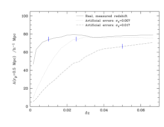
As expected, redshift errors require larger integration limits for a stable estimation. For the artificial redshift errors with $\sigma_{z}=0.007$, it can be located at around $\delta z\approx 0.025$, for the calculation with $\sigma_{z}=0.017$, the maximum is reached at $\delta z\approx 0.05$, that is in both cases at $\delta z\approx 3\sigma_{z}$. From these simulations we conclude that one starts to sample the correlation signal when the integration limits are larger than the Full Width at Half Maximum of the redshift error distribution ($\Delta z=2\sqrt{2\ln 2}\cdot\sigma_{z}\approx 2.3\sigma_{z}$). Thus we conclude that calculate the projected correlation function for the CADIS data, the appropriate choice of the integration limits appears to be $\delta z=\pm 0.05$.

Note that the estimate for the amplitude is systematically lowered in the presence of significant redshift errors. For errors of $\sigma_{z}=0.017$, we find that the maximum amplitude is a factor 1.2 lower than in the case of the unchanged data. For a differential comparison between various redshift intervals a diminished amplitude is in any case no problem, provided one uses the LCRS in its modified form (with artificial redshift errors simulated exaclty as those found in the CADIS survey) as local reference.

4 The evolution of galaxy clustering from $z=1$

4.1 Clustering properties of all galaxies

We calculated the projected correlation function for the CADIS data in three different redshift bins of similar size, $0.2\leq z<0.5$, $0.5\leq z<0.75$, $0.75\leq z\leq 1.07$.

A random catalogue consisting of 30000 randomly distributed “galaxies” was generated for each CADIS field with the same properties as the real data. The surroundings of bright stars in our fields were masked out. The same mask is applied to the random catalogue.

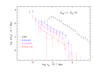
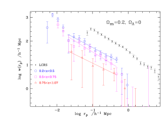
The calculation was carried out for a flat high-density model ($\Omega_{m}=1$, $\Omega_{\Lambda}=0$), a hyperbolic low-density model ($\Omega_{m}=0.2$, $\Omega_{\Lambda}=0$), and a flat low-density model with non-zero comological constant ($\Omega_{m}=0.3$, $\Omega_{\Lambda}=0.7$).

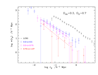
For the CADIS data the projected correlation function $w(r_{p})$ was fitted over the range $0.02\la r_{p}\la 0.5$ $h^{-1}$ Mpc ($-1.7\leq\log r_{p}\leq-0.3$), whereas the LCRS data was fitted in the range $0.07\la r_{p}\la 2h^{-1}$ Mpc ($-1.15\leq\log r_{p}\leq 0.3$), see Figure 3. The fitted amplitudes $A$ at $r_{p}=316h^{-1}$ kpc for CADIS and at $r_{p}=500h^{-1}$ kpc for the LCRS, respectively, and the amplitude of the three-dimensional correlation function at $r_{\mathrm{com}}=1$ Mpc derived from them, are listed in Table 2 (we have left $\gamma$ as a free parameter).

Figure 3: Measured projected correlation function in three redshift bins, for the flat standard model (top), an open model (middle), and for a flat universe with a non-zero cosmological constant (below). Note that the binning in the highest redshift bin is different. Note also that the calculation was carried out in proper coordinates as measured by an observer at the particular redshift under consideration. The lines are the best fits of the data in the indicated range.

Although we correct for the missing variance on large scales by adding the estimated integral constraint ${\cal I}$ to the measured amplitudes, cosmic variance may still play a rôle. However, as can be seen from Figure 4, the errors of the weighted mean of the correlation function (if at all) only slightly underestimate the varying clustering strength measured in each single field. In Figure 4 we show the amplitudes $A$ of the projected correlation function at $r_{p}=0.316h^{-1}$ Mpc measured in each individual field (no integral constraints are added yet), for the bright galaxies in the lowest redshift bin, for $\Omega_{m}=0.3$, $\Omega_{\Lambda}=0.7$.

Figure 4: The amplitudes of the projected correlation function at $r_{p}=0.316h^{-1}$ Mpc estimated in each individual field, for the bright galaxies in the lowest redshift bin, for $\Omega_{m}=0.3$, $\Omega_{\Lambda}=0.7$. The solid line is the amplitude measured from the weighted mean, the dotted lines are the $1\sigma$. levels

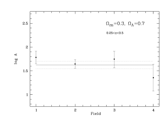
The solid line is the amplitude measured from the weighted mean, the dotted lines are the $1\sigma$ levels. The spread of the measured values around the mean is reasonably small, and within their errors they lie within the error of the weighted mean.

Although the projected distances at which the amplitudes are fitted are still close to the largest separations measured, the measured amplitude $A$ and the slope $\gamma$ are independent, the error $\sigma_{\gamma}$ is negligible, and therefore the second term in equation (13) is negligible. Then

$$\sigma_{\log\xi_{1\mathrm{Mpc}}}=\frac{\partial\log\xi_{1\mathrm{Mpc}}}{\partial\log w(r_{p})}\cdot\sigma_{\log w(r_{p})}\leavevmode\nobreak\ .$$ (26)

From equation (12) we find $\frac{\partial\log\xi_{1\mathrm{Mpc}}}{\partial\log w(r_{p})}=1$, so

$$\sigma_{\log\xi_{1\mathrm{Mpc}}}=\sigma_{\log w(r_{p})}\leavevmode\nobreak\ .$$ (27)

The values of the integral constraint, which are then added to the measured amplitudes of the projected correlation function, are listed in Table 2. The amplitudes of the three-dimensional correlation function at $r_{\rm com}=1$ Mpc are derived from the corrected amplitudes of $w(r_{p})$.

Table 2: The measured amplitude of the projected correlation function in different redshift intervals, at $r_{p}\approx 316h^{-1}$ kpc for CADIS and at $r_{p}\approx 500h^{-1}$ kpc for the LCRS (first lines), respectively, the integral constraint ${\cal I}$ and $\xi_{1\mathrm{Mpc}}$ as calculated from the ${\cal I}$-corrected amplitudes of $w(r_{p})$, for different world models. Numbers in italic indicate that this values are inferred from the LCRS.

Model	$z$ interval		$A$		$\gamma$	${\cal I}$	$\xi_{1\mathrm{Mpc}}$
	0.04$\leq$ $z$	$\leq$ 0.16	71.92$\pm$	${}^{1.83}_{1.79}$	1.92$\pm$0.03	$1.89$	14.06$\pm^{0.35}_{0.34}$
$\Omega_{m}=1.0$	$0.2\leq$ $z$	$<0.5$	$17.27$$\pm$	${}^{2.34}_{2.06}$	$1.83\pm 0.09$	$5.53$	$4.23\pm^{0.43}_{0.38}$
$\Omega_{\Lambda}=0$	$0.5\leq$ $z$	$<0.75$	$9.16$$\pm$	${}^{2.01}_{1.65}$	$1.89\pm 0.14$	$3.20$	$3.26\pm^{0.53}_{0.43}$
	$0.75\leq$ $z$	$<1.07$	$3.88$$\pm$	${}^{1.31}_{0.98}$	$2.03\pm 0.18$	$1.06$	$1.82\pm^{0.48}_{0.36}$
	0.04$\leq$ $z$	$\leq$ 0.1	73.12$\pm$	${}^{1.91}_{1.87}$	1.93$\pm$0.03	$1.88$	14.19$\pm^{0.36}_{0.35}$
$\Omega_{m}=0.2$	$0.2\leq$ $z$	$<0.5$	$21.44$$\pm$	${}^{2.79}_{2.47}$	$1.80\pm 0.09$	$6.66$	$5.39\pm^{0.52}_{0.45}$
$\Omega_{\Lambda}=0$	$0.5\leq$ $z$	$<0.75$	$12.20$$\pm$	${}^{2.55}_{2.11}$	$1.92\pm 0.14$	$3.69$	$4.20\pm^{0.67}_{0.56}$
	$0.75\leq$ $z$	$<1.07$	$5.01$$\pm$	${}^{1.81}_{1.33}$	$1.97\pm 0.22$	$1.30$	$2.31\pm^{0.66}_{0.48}$
	0.04$\leq$ $z$	$\leq$ 0.16	79.48$\pm$	${}^{2.00}_{1.95}$	1.91$\pm$0.03	$1.89$	15.49$\pm^{0.39}_{0.37}$
$\Omega_{m}=0.3$	$0.2\leq$ $z$	$<0.5$	$23.40$$\pm$	${}^{3.42}_{2.98}$	$1.85\pm 0.10$	$6.30$	$5.52\pm^{0.63}_{0.55}$
$\Omega_{\Lambda}=0.7$	$0.5\leq$ $z$	$<0.75$	$15.72$$\pm$	${}^{3.28}_{2.71}$	$1.97\pm 0.13$	$4.30$	$5.31\pm^{0.87}_{0.72}$
	$0.75\leq$ $z$	$<1.07$	$6.19$$\pm$	${}^{2.78}_{1.92}$	$2.11\pm 0.25$	$1.33$	$2.81\pm^{1.04}_{0.72}$

4.2 Clustering evolution of bright galaxies

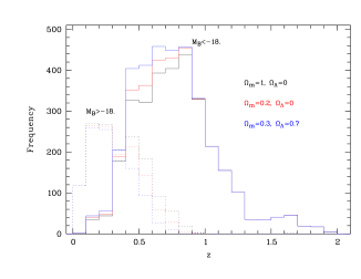
It is well known that in the local universe bright galaxies are much more strongly clustered than faint ones (Norberg et al. 2002), as expected if bright (massive) galaxies form in the high density peaks of the underlying dark matter density field (Kaiser 1984). For a reliable determination of clustering evolution galaxies with similar absolute luminosities have to be compared. Based on the photometry between $400$ and $1250$ nm the absolute $B$-band luminosities can be determined directly without any $K$-correction uncertainty. At redshifts up to $z\sim 0.3$ CADIS is dominated by faint ($M_{B}<-18+5\log h$) galaxies (see Figure 5), which supress the correlation signal and distort the measurement of the clustering evolution. A consistent comparison of galaxy clustering at different redshifts can be achieved, if we calculate the correlation function in the lowest two redshift bins only for galaxies brighter than $M_{B}=-18+5\log h$. For this purpose, the lowest redshift bin has to be confined to $z\geq 0.25$ instead of $z=0.2$, because there are only very few bright galaxies at redshifts smaller than 0.3. At $z=1.07$ the magnitude limit is slightly fainter ($M_{B}\la-18.6+5\log h$).

Figure 5: Redshift distribution of faint ($M_{B}>-18+5\log h$) and bright ($M_{B}\leq-18+5\log h$) galaxies, for the different cosmologies under consideration in this work.

The amplitudes of $w(r_{p})$ and $\xi_{1\mathrm{Mpc}}$ are given in Table 3.

Table 3: The measured amplitude of the projected correlation function at $r_{p}\approx 316h^{-1}$ kpc for the bright ($M_{B}\leq-18+5\log h$) galaxies, the integral constraint ${\cal I}$, and $\xi_{1\mathrm{Mpc}}$, calculated from the ${\cal I}$-corrected $A$, for different world models. Note that for the bright sample the calculation for the first redshift bin was started at $z=0.25$ instead of $z=0.2$, because there are only very few bright galaxies at redshifts smaller than 0.3.

Model	$z$ interval		$A$		$\gamma$	${\cal I}$	$\xi_{1\mathrm{Mpc}}$
	$0.25\leq$ $z$	$<0.5$	$27.38$$\pm$	${}^{5.31}_{4.45}$	$1.98\pm 0.14$	$8.26$	$6.80\pm^{1.02}_{0.85}$
$\Omega_{m}=1$	$0.5\leq$ $z$	$<0.75$	$11.14$$\pm$	${}^{3.27}_{2.53}$	$2.02\pm 0.19$	$4.12$	$4.05\pm^{0.87}_{0.67}$
$\Omega_{\Lambda}=0$	$0.75\leq$ $z$	$\leq 1.07$	$3.88$$\pm$	${}^{1.31}_{0.98}$	$2.03\pm 0.18$	$1.06$	$1.82\pm^{0.48}_{0.36}$
	$0.25\leq$ $z$	$<0.5$	$31.50$$\pm$	${}^{6.55}_{5.42}$	$1.85\pm 0.17$	$10.24$	$8.02\pm^{1.26}_{1.04}$
$\Omega_{m}=0.2$	$0.5\leq$ $z$	$<0.75$	$15.42$$\pm$	${}^{3.98}_{3.16}$	$2.02\pm 0.16$	$4.66$	$5.34\pm^{1.06}_{0.84}$
$\Omega_{\Lambda}=0$	$0.75\leq$ $z$	$\leq 1.07$	$5.01$$\pm$	${}^{1.81}_{1.33}$	$1.97\pm 0.22$	$1.30$	$2.31\pm^{0.66}_{0.48}$
	$0.25\leq$ $z$	$<0.5$	$39.46$$\pm$	${}^{8.15}_{6.76}$	$1.83\pm 0.18$	$12.74$	$10.01\pm^{1.57}_{1.29}$
$\Omega_{m}=0.3$	$0.5\leq$ $z$	$<0.75$	$22.21$$\pm$	${}^{5.27}_{4.26}$	$2.00\pm 0.16$	$5.85$	$7.23\pm^{1.40}_{1.13}$
$\Omega_{\Lambda}=0.7$	$0.75\leq$ $z$	$\leq 1.07$	$6.19$$\pm$	${}^{2.78}_{1.92}$	$2.11\pm 0.25$	$1.33$	$2.81\pm^{1.04}_{0.72}$

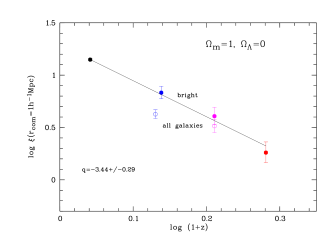
We parameterise the evolution of the clustering strength with redshift by a parameter $q$, which gives directly the deviation of the evolution from the global Hubble flow:

$$\xi_{1\mathrm{Mpc}}=\xi_{0}(1+z)^{q}\leavevmode\nobreak\ ,$$ (28)

thus the parameter $q$ can be deduced from a straight line fit in a $\log\xi$–$\log(1+z)$ plot (see Figure 6). $q=-2$ is expected in case of linear clustering growth. For the flat high-density model we find $q=-3.44\pm 0.29$, for the open model we find $-2.84\pm 0.30$, and for the model with non-zero cosmological constant $q=-2.28\pm 0.31$.

The data point of the LCRS is included in the fit for $q$. Its error is extremely small compared to the CADIS data, and thus it dominates the fit. If we exclude the LCRS from the fit, we get $q=3.86\pm 0.80$, $q=3.52\pm 0.84$, and $q=3.12\pm 0.90$ (cosmologies in the same order as above). The slopes are systematically steeper, although still the same within their errors. However, the reduced $\chi^{2}$ of the fits including the LCRS is smaller than that without. We regard this as a corroboration that the connection to the local universe indeed improves the determination of $q$.

Figure 6: The evolution of the clustering strength (the amplitude of the three-dimensional correlation function at at a comoving separation of $1h^{-1}$ Mpc) with redshift. The integral constraint ${\cal I}$ has been taken into account. Filled symbols are only bright galaxies, open symbols include the complete sample. The line is the fit to the bright galaxies, the first data point (from the LCRS) is included in the fit.

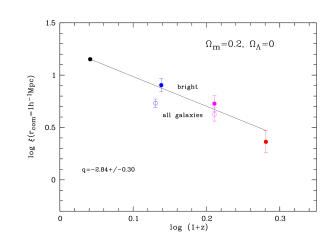
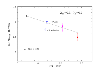
The dependency of the parameter $q$ on the cosmology chosen for the calculation is as follows: The estimate of $w(r_{p})$ as calculated from equation (22) is the product of $\zeta_{\mathrm{esti}}(r_{p})$ (as defined in equation (21)), and the integral given in equation (23). The physical distances $r_{p}$ are stretched (or compressed, respectively) corresponding to the cosmology, that means the individual histograms $\langle DD\rangle$, $\langle RR\rangle$ and $\langle RD\rangle$ are shifted along the $r_{p}$ axis. However, the estimator $\zeta_{\mathrm{esti}}(r_{p})$ is unaffected, because all histograms are shifted in the same way. The integral $\Delta r_{\parallel}$ of course changes with cosmology, thus the dependence of the amplitude of the projected correlation function on cosmology is due to the integration along the line of sight. Since we fit always at the same physical scale ($r_{p}=316h^{-1}$ kpc for CADIS), the values of $\xi_{1\mathrm{Mpc}}$ we deduce from $w(r_{p})$ show the same dependency on cosmology. The differences in $\Delta r_{\parallel}$ are increasing with increasing redshift. At our highest redshift bin ($\langle z\rangle=0.91$) we expect $\frac{\Delta r_{\parallel}(\Omega_{m}=0.3,\Omega_{\Lambda}=0.7)}{\Delta r_{\parallel}(\Omega_{m}=1,\Omega_{\Lambda}=0)}\approx 1.6$, hence we expect (and find) the amplitudes of the correlation function to differ by the same factor. The integral constraint only depends on the measured correlation function (see equations (15) to (17). It is, though estimated with large errors in the highest redshift bin, of the order of 25% of the measured amplitude at $316h^{-1}$ kpc in all cosmologies, thus this additional offset does not change the ratio of the amplitudes in different cosmologies. If we consider the “local” measurement not to change with cosmology, than we expect the parameter $q$ to change (due to the change in $\xi_{1\mathrm{Mpc}}$ at the highest redshift bin) by $\Delta q=\frac{\log 1.6}{\log 1.91-\log 1.1}=0.93$ between the matter-dominated flat cosmology and the flat cosmology with non-zero cosmological constant. We find $\Delta q=1.16$. The slightly larger difference measured by us is caused by the bin at $\langle z\rangle=0.625$ (see Figure 6.

4.3 Comparison with other work

Before analysing the $SED$ type dependent evolution of galaxy clustering, we compare our results with previous attempts to study the clustering evolution with redshift. In the literature there are essentially only two investigations of the evolution of galaxy clustering, that can be compared with the present work: one analysis by Le Fèvre et al. (1996) which has been carried out in the framework of the Canada France Redshift Survey (in the following CFRS), and one by Carlberg et al. (2000), done on the CNOC sample (Canadian Network for Observational Cosmology).

Le Fèvre et al. (1996) used the projected correlation function to investigate the spatial clustering of 591 galaxies between $0.2\leq z\la 1.1$, in five CFRS fields (for a description of the survey see Lilly et al. (1995) and Schade et al. (1995), respectively) of approximately the same size as our CADIS fields. The objects are primarily located in three parallel strips for each of the five fields, within which almost 100% spectroscopic sampling was obtained, separated by regions where few spectroscopic observations were carried out. The galaxies with spectroscopic redshifts have $I\leq 22.5^{\mathrm{mag}}$. They computed the projected correlation function in three redshift bins between $0.2\leq z\leq 0.5$, $0.5\leq z\leq 0.75$, and $0.75\leq z\leq 1.0$, with integration limits of $\delta_{z}=\pm 0.0075$. For the connection to $z=0$ they took values of $r_{0}(z=0)$ from Loveday et al. (1995) and Hudon & Lilly (1996).

Figure 7 shows the amplitude of the three dimensional correlation function at $r_{\rm com}=1h^{-1}$ Mpc, deduced from the projected correlation function, in comparison with our own data. Since they did not apply corrections for the missing variance, we calculated $\xi_{1\mathrm{Mpc}}$ without adding ${\cal I}$ to the measured amplitudes of $w(r_{p})$. For direct comparison, we have to multiply our measured amplitudes of the projected correlation function of the complete sample by $\frac{A(\delta z=0.01)}{A(\delta z=0.05)}=1.2$ in order to allow for the large errors of the CADIS multicolour redshifts (see Section 3).

Figure 7: The amplitudes of the three dimensional correlation function at $r_{\rm com}=1h^{-1}$ Mpc, deduced from the projected correlation function of the CFRS data (crosses), in comparison with our own data (open symbols). The amplitudes are calculated without taking the integral constraint into account, to allow for a direct comparison with the data of Le Fèvre et al. (1996). The data points with integral constraint correction can be seen in Figure 6 for comparison. The filled symbols are our data points corrected for the influence of the redshift errors on the amplitude of the projected correlation function (shifted by a factor of 1.2). The dotted line is the fit of the CFRS data points including the value of $r_{0}(z=0)$ from Loveday et al. (1995). It seems that they underestimated the errors, since from a sample of roughly six times fewer galaxies they derived errors of the same size as ours.

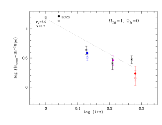
With this correction, the CFRS data points are consistent with our own measurement for the sample as a whole. However, it seems that they underestimated the errors, since from a sample of roughly six times less galaxies they derived errors of the same size as ours.

Le Fèvre et al. (1996) claim that if $r_{0}(z=0)=5h^{-1}$ Mpc, $0<\epsilon\la 2$. The fit of their data points, including a direct connection to $z=0$, that does not take the different properties of the samples into account, formally yields $q=-3.04\pm 0.21$. If the connection to $z=0$ is disregarded, we find $q=-1.18\pm 0.63$ from their data.

This exercise shows that the value of $q$ derived from the CFRS solely depends on the connection to the present epoch. To deduce a reliable result, it is indispensable to take into account that the catalogues to be compared have to consist of the same mix of Hubble types and luminosities, as we have seen, bright galaxies are more strongly clustered. It is not possible to estimate the evolution of the clustering strength by comparing a sample of intrinsically faint galaxies at redshifts $z\ga 0.3$ with the bright galaxies which dominate the local measurements. The comparison between different samples has to be carried out in a selfconsistent way. The integral constraint, which they did not take into account, is different in different redshift intervals (see Table 2), and thus alters the result. Also the measured amplitude of the projected correlation function depends on the redshift accuracy and the appropriate choice of the integration limits.

Thus we conclude that their measurement is consistent with ours, but they did not treat the local measurement selfconsistently.

Carlberg et al. (2000) carried out an analysis of the clustering evolution on a sample of 2300 bright galaxies from the CNOC survey. The survey itself is described in detail in Yee et al. (1996). The galaxies have $k$-corrected and evolution-compensated $R$ luminosities $M_{R}^{k,e}<-20^{\mathrm{mag}}$ ($H_{0}=100$ km s^-1). The redshift distribution extends to $z=0.65$. For comparison with $z=0$, they selected a comparable sample from the LCRS. They also do not apply corrections for the integral constraint, but since the survey area of the CNOC is large (extending over $1.55\leavevmode\nobreak\ \squareforqed\degr$ in total) ${\cal I}$ is expected to be negligible at the scales they investigate ($0.16\leq r_{p}\leq 5.0h^{-1}$ Mpc). The parameter $\epsilon$ (see Groth & Peebles 1977; Efstathiou et al. 1991) that they use for the parametrisation of the clustering evolution can of course be related to the parameter $q$

$$q=-(3+\epsilon-\gamma)\leavevmode\nobreak\ .$$ (29)

With equation (29) we can calculate the parameters $q$ which correspond to the $\epsilon$ values they give: They found $q=-2.00\pm 0.22$ for $\Omega_{m}=1$, $\Omega_{\Lambda}=0$, $q=-1.37\pm 0.18$ for $\Omega_{m}=0.2$, $\Omega_{\Lambda}=0$, and $q=-0.39\pm 0.19$ for $\Omega_{m}=0.2$, $\Omega_{\Lambda}=0.8$.

Their values indicate a much slower evolution of the clustering than our results. The reason for the descrepancy might be the different sample selection – the CNOC galaxies have been selected to be bright in the $R$ band, whereas the galaxies in our sample have bright blue luminosities. As we will show in the next section, the clustering growth of blue and red galaxies evolves differently, and in fact the $q$ values we derived for our subsample of early type galaxies are within the errors identical with the values estimated by Carlberg et al. (2000).

4.4 The evolution of the correlation function for different Hubble types

Various local surveys have established that the red galaxies are much more strongly clustered than the blue ones (Davis & Geller 1976; Lahav & Saslaw 1992; Santiago & Strauss 1992; Iovino et al. 1993; Hermit et al. 1996; Guzzo et al. 1997; Willmer et al. 1998).

Le Fèvre et al. (1996) separated their sample into red and blue galaxies (bluer and redder than the Coleman et al. (1980) Sbc spectral energy distribution), and found that they have comparable clustering amplitues at $z>0.5$. Here we show that this is not the case, at redshifts $z\ga 0.2$ red galaxies are more strongly clustered than blue ones.

The galaxy library used for the multicolour classification resembles regular grids in redshift and SED, thus the Hubble type can also be estimated from the observations. This enables us to investigate the evolution of the clustering of different populations of galaxies.

We devided the sample into two SED bins, with $SED\leq 60$, including galaxy types E to Sbc (1355 galaxies), and $SED>60$, including Sds to Starbursts (2311 galaxies), respectively. Galaxies with earlier $SED$s have smaller redshift errors, therefore we primarily concentrate on the investigation of the evolution of the large scale structure of the galaxies in the $SED\leq 60$ sample.

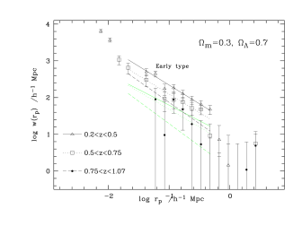
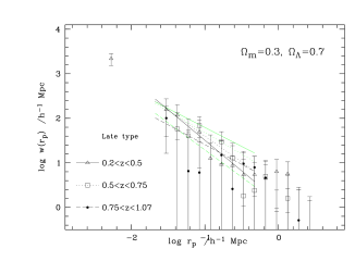
Figure 8 shows $w(r_{p})$ for the different redshift bins, in comparison with the projected correlation function of all galaxies, for a flat $\Omega_{\Lambda}=0.7$ model. The early type galaxies show significantly stronger clustering than the late types. Table 4 lists the amplitudes at $r_{p}=316h^{-1}$ kpc, fitted between $\sim 20h^{-1}$ kpc and $\sim 500h^{-1}$ kpc, and the integral constraint ${\cal I}$.

Figure 8: The projected correlation function in three different redshift bins; upper panel: early type galaxies in comparison with all galaxies (only the fits are shown as grey lines), lower panel: late type galaxies in comparison with all galaxies for $\Omega_{m}=0.3$, $\Omega_{\Lambda}=0.7$.

Table 4: The measured amplitude of the projected correlation function at $r_{p}=316h^{-1}$ kpc and the integral constraint ${\cal I}$, in different redshift intervals for two SED bins, for different world models.

Model	$z$ interval		$A(SED\leq 60)$		$\gamma$	${\cal I}$	$A(SED>60)$		$\gamma$	${\cal I}$
	$0.2\leq$ z	$<0.5$	$46.67$ $\pm$	${}^{6.11}_{5.40}$	$1.95\pm 0.09$	$14.33$	$7.80$ $\pm$	${}^{3.26}_{2,30}$	$1.96\pm 0.24$	$0.14$
$\Omega_{m}=1.0$	$0.5\leq$ z	$<0.75$	$21.33$ $\pm$	${}^{4.40}_{3.64}$	$2.13\pm 0.14$	$6.12$	$4.97$ $\pm$	${}^{2.94}_{1.85}$	$2.01\pm 0.33$	$0.66$
$\Omega_{\Lambda}=0$	$0.75\leq$ z	$<1.07$	$5.53$ $\pm$	${}^{9.00}_{3.42}$	$2.84\pm 0.93$	$1.01$	$4.78$ $\pm$	${}^{1.96}_{1.39}$	$1.98\pm 0.22$	$0.57$
	$0.2\leq$ z	$<0.5$	$59.17$ $\pm$	${}^{7.26}_{6.47}$	$1.97\pm 0.09$	$15.59$	$9.09$ $\pm$	${}^{4.01}_{2.78}$	$1.92\pm 0.27$	$2.13$
$\Omega_{m}=0.2$	$0.5\leq$ z	$<0.75$	$27.97$ $\pm$	${}^{5.39}_{4.52}$	$2.01\pm 0.16$	$9.18$	$5.89$ $\pm$	${}^{4.35}_{2.50}$	$2.20\pm 0.44$	$1.31$
$\Omega_{\Lambda}=0$	$0.75\leq$ z	$<1.07$	$11.03$ $\pm$	${}^{10.61}_{5.41}$	$2.69\pm 0.80$	$1.42$	$5.67$ $\pm$	${}^{2.63}_{1.80}$	$0.52\pm 0.86$	–
	$0.2\leq$ z	$<0.5$	$67.60$ $\pm$	${}^{8.47}_{7.53}$	$2.20\pm 0.10$	$15.14$	$6.62$ $\pm$	${}^{4.28}_{2.60}$	$2.37\pm 0.30$	$1.19$
$\Omega_{m}=0.3$	$0.5\leq$ z	$<0.75$	$39.22$ $\pm$	${}^{7.20}_{6.08}$	$2.00\pm 0.11$	$11.12$	$10.40$ $\pm$	${}^{7.13}_{4.23}$	$2.16\pm 0.44$	$2.30$
$\Omega_{\Lambda}=0.7$	$0.75\leq$ z	$<1.07$	$19.53$ $\pm$	${}^{17.36}_{9.19}$	$2.16\pm 0.64$	$3.35$	$9.25$ $\pm$	${}^{3.89}_{2.74}$	$1.89\pm 0.28$	$1.98$

The corresponding amplitudes of the three-dimensional correlation function $\xi(r)$ at a comoving distance of $r_{\rm com}=1h^{-1}$ Mpc, corrected for the missing variance ${\cal I}$, are given in Table 5.

Table 5: The amplitudes of the three-dimensional correlation function $\xi(r)$ at a comoving distance of $r=1$ Mpc, for red ($SED\leq 60$) and blue ($SED>60$) galaxies; the integral constraint has been taken into account in the calculation.

Model	$z$ interval		$\xi_{1\mathrm{Mpc}}$ $(SED\leq 60)$	$\xi_{1\mathrm{Mpc}}$ $(SED>60)$
	$0.2\leq$ z	$<0.5$	$11.26\pm^{1.13}_{1.00}$	$1.46\pm^{0.60}_{0.42}$
$\Omega_{m}=1.0$	$0.5\leq$ z	$<0.75$	$7.27\pm^{1.17}_{0.96}$	$1.49\pm^{0.78}_{0.49}$
$\Omega_{\Lambda}=0$	$0.75\leq$ z	$<1.07$	$2.34\pm^{3.24}_{1.22}$	$1.96\pm^{0.72}_{0.51}$
	$0.2\leq$ z	$<0.5$	$13.77\pm^{1.34}_{1.19}$	$2.08\pm^{0.74}_{0.51}$
$\Omega_{m}=0.2$	$0.5\leq$ z	$<0.75$	$9.87\pm^{1.43}_{1.20}$	$1.89\pm^{1.15}_{0.66}$
$\Omega_{\Lambda}=0$	$0.75\leq$ z	$<1.07$	$4.56\pm^{3.91}_{1.98}$	–
	$0.2\leq$ z	$<0.5$	$15.11\pm^{1.56}_{1.37}$	$1.29\pm^{0.72}_{0.43}$
$\Omega_{m}=0.3$	$0.5\leq$ z	$<0.75$	$13.37\pm^{1.91}_{1.61}$	$3.35\pm^{1.89}_{1.12}$
$\Omega_{\Lambda}=0.7$	$0.75\leq$ z	$<1.07$	$8.57\pm^{6.51}_{3.44}$	$4.01\pm^{1.42}_{0.98}$

Figure 9 shows the amplitudes of the three-dimensional correlation function $\xi(r)$ at a comoving distance of $r=1h^{-1}$ Mpc, for red galaxies ($SED\leq 60$), for $\Omega_{m}=0.3$, $\Omega_{\Lambda}=0.7$. For comparison the data points for the whole sample are also plotted. The amplitudes are corrected for the missing variance ${\cal I}$. The lines are the fits for the $q$-parameter (equation (28)).

Figure 9: The evolution of the clustering strength (at a comoving separation of $1h^{-1}$ Mpc) with redshift, for early type ($SED\leq 60$). The data for the bright galaxies and the complete sample are plotted for comparison. A correction for the integral constraint is included. The first data point (the weighted mean of the LCRS sectors) is not included in the fit for the early type galaxies. We also show the fit which does take it into account (dotted line), and the measurement for the late type sample for the $\Omega_{m}=0.3$, $\Omega_{\Lambda}=0.7$ case. Note that the errors of the late type galaxies are too large to measure the clustering evolution.

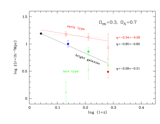
The late type galaxies have large redshift errors, and they are intrinsically only very weakly clustered. Although their number density is high, the large errors and the low correlation signal result in a highly uncertain measurement of their clustering amplitudes (the measurement is shown for the $\Omega_{m}=0.3$, $\Omega_{\Lambda}=0.7$ case), which would make a reliable estimate of the clustering evolution impossible. Also the late type sample is at high redshifts dominated by relatively bright galaxies, whereas at lower redshifts the rather low-mass, fainter galaxies, which are only very weakly clustered, are currently undergoing periods of high starformation rates. A galaxy classified as extreme late type at $z=1$ may have evolved into an Sa at $z=0$, thus we are not dealing with a homogeneous sample. A measurement of the clustering evolution of late type galaxies is therefore not meaningful at this point.

The LCRS measurement is not included in the fits for the early type galaxies. Table 6 lists the parameter $q$ for the early type sample, and compares them to the values found for the bright sample. The evolution of the amplitude of the correlation function is clearly differential, the clustering strength of early type galaxies grows much slower. However, it looks as if the clustering evolution of the CADIS early type sample converges to the same value. In Table 6 we list also the parameter $q$ for the early type sample which was determined when taking the LCRS point into account.

Table 6: The parameter $q$ for early type ($SED\leq 60$) galaxies, for a fit done without taking the the LCRS point into account, and for a fit including it. The evolution of the bright sample is shown for comparison.

Cosmology	$q(SED\leq 60)$, without LCRS	$q(SED\leq 60)$, with LCRS	$q_{\rm bright}$
$\Omega_{m}=1.0$, $\Omega_{\Lambda}=0.0$	$-2.60\pm 0.91$	$-1.52\pm 0.30$	$-3.44\pm 0.29$
$\Omega_{m}=0.2$, $\Omega_{\Lambda}=0.0$	$-2.03\pm 0.82$	$-0.74\pm 0.28$	$-2.84\pm 0.30$
$\Omega_{m}=0.3$, $\Omega_{\Lambda}=0.7$	$-0.85\pm 0.82$	$-0.34\pm 0.28$	$-2.28\pm 0.31$

When the LCRS point (at $z=0.1$) is included in the fit, the CADIS points still lie well on the fitted line, which indicates that the clustering strength of bright and early type galaxies indeed seems to converge to the same point at $z\la 0$.

These values of $q$, $-1.47\pm 0.37$, $-0.71\pm 0.31$, $-0.34\pm 0.32$ (see Table 6 for the corresponding cosmological models) are within their errors identical to the values deduced by Carlberg et al. (2000) from the red CNOC galaxies (they found $q=-2.00\pm 0.22$, $q=-1.37\pm 0.18$, $q=-0.39\pm 0.19$ for the cosmologies in the same order as above, see previous section).

5 Discussion

We now want to discuss the most important results of our present analysis in turn:

(1.) Bright galaxies are more strongly clustered than faint galaxies and show significant growth in clustering since $z\simeq 1$.

At redshifts around $z\approx 0.3$ the CADIS data are dominated by rather faint galaxies, which show smaller clustering amplitudes than brighter ones. On the other hand, the LCRS sample consists mainly of intrinsically bright galaxies. In order to be able to compare our high redshift data self-consistently with the local measurement from the LCRS, we measured the amplitude of the correlation function from a subsample of bright galaxies ($M_{B}\leq-18+5\log h$). We find a significant growth of the clustering strength for this bright subsample:

For the $\Omega_{m},\Omega_{\Lambda}=0.3,0.7$ cosmology we find $q=-2.2$ that is ${\xi_{\rm 1Mpc}(z=0)\over\xi_{\rm 1Mpc}(z=1)}=5.5$. This might be compared with the theoretical predictions by Kauffmann et al. (1999a). They use N-body simulations of dark matter (DM) to derive the clustering of DM halos at $0<z<5$ and semi-analytic models in order to assign a galaxy of certain type and luminosity to each DM halo. Although many properties of their mock galaxies population are only in loose accordance with observations, their result seems robust: the clustering strength of bright galaxies ($M_{B}\leq-19+5\log h$) on 2 Mpc scales follows closely that of the DM halos they are imbedded out to $z\simeq 1$ (bias parameter $\simeq 1$). They find a 3.5-fold increase of $\xi_{\rm 2Mpc}$ between $z=1$ and $z=0$. If one takes into account that the increase should be higher on 1 Mpc scales and that our limit for “bright galaxies” is 1 magnitude fainter (i.e. it includes less massive halos) it seems that the the clustering evolution predicted by $\Lambda$CDM models is in agreement with our measurements.

(2.) At high redshifts, early type galaxies are more strongly clustered than the bright galaxies and the clustering strength of the early type galaxies evolves much more slowly than that of the bright galaxies.

A plausible explanation for the different evolution of the clustering properties of the early type galaxies arises in the context of biased galaxy formation (Bardeen et al. 1986; Brainerd & Villumsen 1994). The first galaxies are born in a highly clustered state, because they form in the bumps and wiggles which are superimposed on the very large-scale density enhancements. The next generations of galaxies form later in the wings of the large-scale enhancements, and are therefore less and less clustered. While the universe expands, the galaxies evolve, age, and eventually merge to form larger, brighter galaxies and ellipticals, and generally add to the population of earlier type galaxies, while new galaxies form at later times in less and less clustered environments. Merging creates galaxies, which suddenly” add to the old population. A merger event also reduces not only the number of galaxies, but also the number of small pair separations in a sample, which reduces the probability of finding pairs of galaxies at small distances – and thus supresses the amplitude of the correlation function. Fried et al. (2001) found the density evolution of the early type and the late type galaxy population in the CADIS galaxy sample suggestive of merging.

Although the clustering strength of the underlying dark matter density field increases with redshift, the biasing decreases. The net effect is a very slowly rising clustering amplitude of the early type (old) galaxies.

Thus, the measured rate of the clustering growth depends on the mixture of galaxy types one observes at different redshifts.

(3.) The evolution of the clustering amplitude of early and bright galaxies converges to the same value at $z\approx 0$.

The convergence of the evolution of the clustering of bright galaxies and galaxies with $SED$s earlier than Sbc towards the same local measurement can also be understood if one takes into account that galaxies evolve and hence the population mix one observes changes with redshifts. The comoving number density of weakly clustered starburst galaxies increases with increasing redshifts, whereas the space density of the highly clustered very early type (E-Sa) galaxies decreases by a factor of $\sim 1.6$ from $z=0$ to $z=1$ (Fried et al. 2001). In our highest redshift bins the clustering signal of the bright subsample is presumably dominated by a weakly clustered population of galaxies, which at that time were bright, and blue. At $z=0$ these weakly clustered blue galaxies have vanished, and now the majority of the early type galaxies (which had later, bluer $SED$s at higher redshifts), are also bright, thus at the present epoch there is a large overlap between the bright and the early type samples. Thus we conclude that the apparent strong growth of clustering of the bright galaxies is dominated by the fading of the unclustered, blue population.

To understand exactly how galaxy evolution influences the measurement of the growth of structure, and the evolution of the large scale structure influences the evolution of galaxies, we need detailed investigations of the evolution of both the correlation function and the luminosity function of galaxies with different $SED$s.

Larger, wide angle deep surveys have only recently become available, and one of them is the COMBO 17 survey (Classifying Objects by Medium-Band Observations in 17 filters, Wolf et al. (2001a)), in some respect the successor of CADIS. The complete catalogue will include $\sim 40000$ galaxies with $I\leq 23$, in 1 ^∘, with $SED$ and morphological information. This amazing data base can be used for various investigations, using the projected correlation function. The higher statistic allows for a more detailed analysis of the evolution of the clustering of different galaxie types and their relation to the underlying dark matter density field.

The clustering properties of starburst galaxies at higher redshifts can be investigated using the emission line galaxies observed by the CADIS emission-line survey using an imaging Fabry-Perot interferometer (Hippelein et al. 2002).These galaxies, which have been detected and classified by their emission lines, have redshifts with an accuracy of 120 km s^-1 – good enough to calculate the three-dimensional correlation function directly. The special observing technique samples galaxies in distinct narrow redshift bins, which allows for the investigation of the evolution of the clustering properties of emission line galaxies between a redshift of $z\approx 1.4$ and $z\approx 0.24$.

The observations have to be compared to theoretical predictions. We plan to carry out a large cosmological simulation including starformation and feedback. The individual galaxies will be assigned an $SED$ according to their stellar masses and starformation histories, so we can perform synthetic photometry applying our CADIS or COMBO 17 filter set to the synthetic spectra. Thus we will be able to “observe” the mock galaxies at different redshifts, and directly compare the simulations to our observations.

References

- Bardeen et al. (1986) Bardeen, J. M., Bond, J. R., Kaiser, N., & Szalay, A. S. 1986, ApJ, 304, 15
- Barrow et al. (1984) Barrow, J. D., Sonoda, D. H., & Bhavsar, S. P. 1984, MNRAS, 210, 19P
- Baugh (1996) Baugh, C. M. 1996, MNRAS, 280, 267
- Bertin & Arnouts (1996) Bertin, E. & Arnouts, S. 1996, A&AS, 117, 393
- Brainerd & Villumsen (1994) Brainerd, T. G. & Villumsen, J. V. 1994, ApJ, 431, 477
- Carlberg et al. (2000) Carlberg, R. G., Yee, H. K. C., Morris, S. L., et al. 2000, ApJ, 542, 57
- Coleman et al. (1980) Coleman, G. D., Wu, C.-C., & Weedman, D. W. 1980, ApJS, 43, 393
- Colless et al. (2001) Colless, M., Dalton, G., Maddox, S., et al. 2001, MNRAS, 328, 1039
- Collins et al. (1992) Collins, C. A., Nichol, R. C., & Lumsden, S. L. 1992, MNRAS, 254, 295
- Connolly et al. (2002) Connolly, A. J., Scranton, R., Johnston, D., et al. 2002, ApJ, 579, 42
- Davis & Geller (1976) Davis, M. & Geller, M. J. 1976, ApJ, 208, 13
- Davis et al. (1982) Davis, M., Huchra, J., Latham, D. W., & Tonry, J. 1982, ApJ, 253, 423
- Davis & Peebles (1983) Davis, M. & Peebles, P. J. E. 1983, ApJ, 267, 465
- Efstathiou et al. (1991) Efstathiou, G., Bernstein, G., Tyson, J. A., Katz, N., & Guhathakurta, P. 1991, ApJ, 380, L47
- Fried et al. (2001) Fried, J. W., von Kuhlmann, B., Meisenheimer, K., et al. 2001, A&A, 367, 788
- Groth & Peebles (1977) Groth, E. J. & Peebles, P. J. E. 1977, ApJ, 217, 385
- Guzzo et al. (1997) Guzzo, L., Strauss, M. A., Fisher, K. B., Giovanelli, R., & Haynes, M. P. 1997, ApJ, 489, 37
- Hauser & Peebles (1973) Hauser, M. G. & Peebles, P. J. E. 1973, ApJ, 185, 757
- Hermit et al. (1996) Hermit, S., Santiago, B. X., Lahav, O., et al. 1996, MNRAS, 283, 709
- Hudon & Lilly (1996) Hudon, J. D. & Lilly, S. J. 1996, ApJ, 469, 519
- Iovino et al. (1993) Iovino, A., Giovanelli, R., Haynes, M., Chincarini, G., & Guzzo, L. 1993, MNRAS, 265, 21
- Kaiser (1984) Kaiser, N. 1984, ApJ, 284, L9
- Kauffmann et al. (1999a) Kauffmann, G., Colberg, J. . M., Diaferio, A., & White, S. D. M. 1999a, MNRAS, 307, 529
- Kauffmann et al. (1999b) Kauffmann, G., Colberg, J. M., Diaferio, A., & White, S. D. M. 1999b, MNRAS, 303, 188
- Kayser et al. (1997) Kayser, R., Helbig, P., & Schramm, T. 1997, A&A, 318, 680
- Kinney et al. (1996) Kinney, A. L., Calzetti, D., Bohlin, R. C., et al. 1996, ApJ, 467, 38
- Lahav & Saslaw (1992) Lahav, O. & Saslaw, W. C. 1992, ApJ, 396, 430
- Landy & Szalay (1993) Landy, S. D. & Szalay, A. S. 1993, ApJ, 412, 64
- Le Fèvre et al. (1996) Le Fèvre, O., Hudon, D., Lilly, S. J., et al. 1996, ApJ, 461, 534
- Lilly et al. (1995) Lilly, S. J., Le Fevre, O., Crampton, D., Hammer, F., & Tresse, L. 1995, ApJ, 455, 50
- Limber (1954) Limber, D. N. 1954, ApJ, 119, 655
- Loveday et al. (1995) Loveday, J., Maddox, S. J., Efstathiou, G., & Peterson, B. A. 1995, ApJ, 442, 457
- Maddox et al. (1990) Maddox, S. J., Efstathiou, G., Sutherland, W. J., & Loveday, J. 1990, MNRAS, 242, 43P
- Meisenheimer et al. (2002) Meisenheimer, K., Fried, J., Hippelein, H., et al. 2002, A&A, 00, 000
- Meisenheimer & Röser (1986) Meisenheimer, K. & Röser, H.-J. 1986, in Use of CCD Detectors in Astronomy, Baluteau J.-P. and D’Odorico S., (eds.), 227
- Norberg et al. (2002) Norberg, P., Baugh, C. M., Hawkins, E., et al. 2002, MNRAS, 332, 827
- Oke (1990) Oke, J. B. 1990, AJ, 99, 1621
- Peebles (1973) Peebles, P. J. E. 1973, ApJ, 185, 413
- Peebles (1974) —. 1974, ApJS, 28, 37
- Peebles (1975) —. 1975, ApJ, 196, 647
- Peebles & Groth (1975) Peebles, P. J. E. & Groth, E. J. 1975, ApJ, 196, 1
- Peebles & Hauser (1974) Peebles, P. J. E. & Hauser, M. G. 1974, ApJS, 28, 19
- Phillipps et al. (1978) Phillipps, S., Fong, R., Fall, R. S. E. S. M., & MacGillivray, H. T. 1978, MNRAS, 182, 673
- Röser & Meisenheimer (1991) Röser, H. . & Meisenheimer, K. 1991, A&A, 252, 458
- Santiago & Strauss (1992) Santiago, B. X. & Strauss, M. A. 1992, ApJ, 387, 9
- Schade et al. (1995) Schade, D., Lilly, S. J., Crampton, D., et al. 1995, ApJ, 451, L1
- Shectman et al. (1996) Shectman, S. A., Landy, S. D., Oemler, A., et al. 1996, ApJ, 470, 172
- Stoughton et al. (2002) Stoughton, C., Lupton, R. H., Bernardi, M., Blanton, M. R., & Burles, S. 2002, AJ, 123, 485
- Totsuji & Kihara (1969) Totsuji, H. & Kihara, T. 1969, PASJ, 21, 221
- Walsh (1995) Walsh, J. 1995, http://www.eso.org/observing/standards/spectra
- Willmer et al. (1998) Willmer, C. N. A., da Costa, L. N., & Pellegrini, P. S. 1998, AJ, 115, 869
- Wolf et al. (2001a) Wolf, C., Dye, S., Kleinheinrich, M., et al. 2001a, A&A, 377, 442
- Wolf et al. (2001b) Wolf, C., Meisenheimer, K., & Röser, H. . 2001b, A&A, 365, 660
- Wolf et al. (2001c) Wolf, C., Meisenheimer, K., Röser, H. ., et al. 2001c, A&A, 365, 681
- Yee et al. (1996) Yee, H. K. C., Ellingson, E., & Carlberg, R. G. 1996, ApJS, 102, 269
- York et al. (2000) York, D. G., Adelman, J., Anderson, J. E., et al. 2000, AJ, 120, 1579
- Zehavi et al. (2002a) Zehavi, I., Blanton, M. R., Frieman, J. A., et al. 2002a, ApJ, 571, 172
- Zehavi et al. (2002b) Zehavi, I., Weinberg, D. H., Zheng, Z., et al. 2002b, astro-ph/0301280, 000, 00