The X-ray and extreme-ultraviolet flux evolution of SS Cygni throughout outburst

Abstract

We present the most complete multiwavelength coverage of any dwarf nova outburst: simultaneous optical, Extreme Ultraviolet Explorer, and Rossi X-ray Timing Explorer observations of SS Cygni throughout a narrow asymmetric outburst. Our data show that the high-energy outburst begins in the X-ray waveband 0.9–1.4 d after the beginning of the optical rise and 0.6 d before the extreme-ultraviolet rise. The X-ray flux drops suddenly, immediately before the extreme-ultraviolet flux rise, supporting the view that both components arise in the boundary layer between the accretion disc and white dwarf surface. The early rise of the X-ray flux shows the propagation time of the outburst heating wave may have been previously overestimated.

The transitions between X-ray and extreme-ultraviolet dominated emission are accompanied by intense variability in the X-ray flux, with timescales of minutes. As detailed by Mauche & Robinson, dwarf nova oscillations are detected throughout the extreme-ultraviolet outburst, but we find they are absent from the X-ray lightcurve.

X-ray and extreme-ultraviolet luminosities imply accretion rates of $3\times 10^{15}\,\rm g\,s^{-1}$ in quiescence, $1\times 10^{16}\,\rm g\,s^{-1}$ when the boundary layer becomes optically thick, and $\sim 10^{18}\,\rm g\,s^{-1}$ at the peak of the outburst. The quiescent accretion rate is two and a half orders of magnitude higher than predicted by the standard disc instability model, and we suggest this may be because the inner accretion disc in SS Cyg is in a permanent outburst state.

1 Introduction

Dwarf novae are remarkable binary stars that exhibit frequent large-amplitude optical outbursts. They are relatively bright objects and their optical lightcurves have been studied in detail by amateur astronomers for more than a century. Figure 1 shows a fragment of this coverage of the brightest dwarf nova, SS Cygni.

Figure 1: Two-and-a-half year portion of the AAVSO visual lightcurve of SS Cygni. The outburst discussed in this paper is centred on JD 2 450 370.

The outburst behaviour of dwarf novae has been interpreted as the result of a thermal-viscous instability in the accretion disc surrounding the white dwarf primary star [Osaki¡1974¿, Meyer & Meyer-Hofmeister¡1981¿, Bath & Pringle¡1982¿]. The disc instability model has been developed over many years (e.g. ?; ?; ?) and though it has tended to lack predictive power, the model now accounts reasonably well for the observed optical lightcurves. A recent review of its strengths and weaknesses is given by ?.

Optical lightcurves of dwarf novae provide a reasonably good indicator of the behaviour of the outer accretion disc, which has temperatures in the range $10^{3}$–$10^{4}$ K. They tell us little, however, about the inner disc and boundary layer where most of the gravitational energy is believed to be released. The boundary layer is the region between the disc and the star where disc material loses kinetic energy and settles onto the white dwarf surface. Temperatures of $10^{5}$-$10^{8}$ K are generated in this region, so it must be studied in the extreme-ultraviolet and X-ray wavebands. Observations in these wavebands allow us to investigate the energetics of dwarf nova outbursts and, in principle, can provide a clean probe of the mass transfer rate through the boundary layer onto the white dwarf. This is a key measurement for comparison with accretion disc models.

Unfortunately, high-energy observations are rare because the unpredictable nature of dwarf nova outbursts make them difficult targets for space-based observatories, which tend to be scheduled weeks or months in advance. The duration of dwarf nova outbursts is also a problem because, lasting typically for a week, they are too long to be covered by a normal pointed observation and too short for repeated monitoring observations to be efficient.

Some of the best high-energy coverage of dwarf nova outbursts to date is that obtained with the early scanning X-ray experiments. Despite poor signal-to-noise ratio, these instruments scanned the same regions of sky many times over long baselines and the resulting coverage was well suited to the outbursts of dwarf novae. In particular, SS Cyg was well observed with Ariel V [Ricketts, King & Raine¡1979¿] and U Gem with HEAO 1 [Mason et al.¡1978¿, Swank et al.¡1978¿]. EXOSAT observations with higher signal-to-noise ratio but worse temporal coverage were made of SS Cyg [Jones & Watson¡1992¿], VW Hyi [Pringle et al.¡1987¿] and U Gem [Mason et al.¡1988¿]. More recently, the ROSAT all-sky survey provided the first combination of good sensitivity and temporal coverage, resulting in relatively well-sampled outburst observations of SS Cyg [Ponman et al.¡1995¿], VW Hyi [Wheatley et al.¡1996b¿], and Z Cam [Wheatley et al.¡1996a¿]. ROSAT was also used to monitor the dwarf nova YZ Cnc [Verbunt, Wheatley & Mattei¡1999¿].

EXOSAT and ROSAT had some sensitivity to the extreme-ultraviolet waveband, but more recently the Extreme Ultraviolet Explorer (EUVE) has provided the first detailed view of dwarf nova outbursts in the extreme-ultraviolet. Rapid-response target-of-opportunity observations allowed EUVE to observe the earliest moments of the extreme-ultraviolet outburst. Observations were made of SS Cyg [Mauche, Raymond & Mattei¡1995¿], U Gem [Long et al.¡1996¿], VW Hyi [Mauche¡1996¿] and OY Car [Mauche & Raymond¡2000¿]. ? discuss all these observations and find that extreme-ultraviolet flux rises dramatically 0.7–1.5 d after the initial optical rise. It peaks with or slightly after the optical, declines gradually for a few days, and then declines more steeply than the optical emission.

While the extreme-ultraviolet behaviour of dwarf nova outbursts is now well documented, the X-ray picture remains fragmentary and the individual observations listed above yield only a sketchy picture of the X-ray behaviour of dwarf novae through outburst. The overall picture that emerges is that hard X-rays are present in quiescence, but strongly suppressed during outburst (with the exception of U Gem; ?). The X-ray suppression is approximately coincident with the sharp rise in the extreme-ultraviolet, and the X-ray flux remains low (but non-zero) throughout outburst until it recovers suddenly at the very end of the optical outburst.

? and ? suggest the transition from X-ray to extreme-ultraviolet emission occurs when the rising accretion rate causes the boundary layer to become optically-thick to its own radiation. It then cools efficiently and the optically-thin hard X-ray emission (kT$\sim$10 keV) is replaced by intense optically-thick extreme-ultraviolet emission (kT$\sim$10 eV).

This overall picture is consistent with most of the existing observations, but the various individual features have never been observed together in a single dwarf nova outburst. In this paper we present very long observations, in both the X-ray and extreme-ultraviolet wavebands, covering a full dwarf nova outburst of SS Cyg. We employ simultaneous target-of-opportunity observations with EUVE and the Rossi X-ray Timing Explorer (RXTE), triggered by amateur astronomers, to provide the most complete multiwavelength coverage of any dwarf nova outburst.

2 Observations

2.1 Optical

The American Association of Variable Star Observers (AAVSO) routinely monitor a large number of variable stars, mainly visually with small telescopes. In May 1996 we issued a request in AAVSO Alert Notice 221 [Mattei¡1996a¿] to monitor SS Cyg particularly intensely in preparation for our pre-approved target-of-opportunity observations with RXTE  and EUVE. We issued further requests in June and September in AAVSO Alert Notices 222, and 229 [Mattei¡1996b¿, Mattei¡1996c¿] and finally on 1996 October 9 we were able to trigger our satellite observations. At 03:45 UT an AAVSO observer in California, Tom Burrows, warned us that SS Cyg was probably on the rise at $\rm m_{vis}$=11.5 and this was confirmed at 06:45 UT by an observer in Hawaii, Bill Albrecht, at which point it had reached $\rm m_{vis}$=10.9. We triggered our RXTE and EUVE observations at around 07:15 UT.

The AAVSO lightcurve of SS Cyg [Mattei, Saladyga & Waagen¡1985¿] is an invaluable resource, with a continuous record of observations dating back to the discovery of the system in 1896 [Pickering & Fleming¡1896¿]. Figure 1 shows the AAVSO lightcurve of SS Cyg for 2.5 yrs around the time of our RXTE and EUVE observations.

The outburst properties of SS Cyg are analysed and discussed by ? and ?. They find the outburst durations of SS Cyg form a bimodal distribution with peaks at one and two weeks. The decay timescales of all outbursts are similar, around 2.4 d mag^-1, but rise timescales range from 0.5–3.5 d mag^-1. The outburst covered by our X-ray and extreme-ultraviolet observations is narrow with a fast rise.

2.2 X-ray

RXTE observations of SS Cyg began at 1996 October 9 16:47 UT, less than ten hours after our trigger. We observed continuously for two days in an attempt to cover the expected transition from dominant X-ray to extreme-ultraviolet emission, and for three days at the end of the outburst in an attempt to cover the reverse transition. Total exposure times were 118 ks and 175 ks respectively, with gaps due only to Earth occultations and passage of the spacecraft through the South Atlantic Anomaly.

We use data from the proportional counter array (PCA), which consists of five xenon-filled proportional counter units (PCUs) labeled 0 to 4. PCUs 3 and 4 are often switched off due to discharge problems and so we use only PCUs 0–2 for the lightcurves presented here. All RXTE count rates in this paper are for three PCUs. For hardness ratios we use all five PCUs where available in order to maximise the signal-to-noise ratio. We extract data only from the top xenon layer of each PCU and accumulate lightcurves in the energy range 2.3–15.2 keV corresponding to PCA pulse height analysis (PHA) channels 5–41. For hardness ratios we split the lightcurves at PHA channel 15 (5.8 keV).

For lightcurves we exclude data only if the elevation about the Earth’s limb is less than 3 deg. For spectra we exclude data where the elevation is less than 10 deg, and also for 30 min after passage through the South Atlantic Anomaly and whenever the electron contamination is $>$10%. We background subtract our data using the faint source (L7/240) background model.

2.3 Extreme ultraviolet

EUVE [Bowyer & Malina¡1991¿, Bowyer et al.¡1994¿] observations of SS Cyg began on 1996 October 9 21:39 UT and were performed continuously for 13 days. EUVE data are acquired only during satellite night, which comes around every 95 min and lasted during our observation for between 23 min and 32 min. Valid data are collected during intervals when various satellite housekeeping monitors (including detector background and primbsch/deadtime corrections) are within certain bounds. After discarding numerous short ($\Delta t\leq 10$ min) data intervals comprising less than 10% of the total exposure, we were left with a net exposure of 208 ks. Unfortunately, the Deep Survey (DS) photometer was switched off between October 11 8:46 UT and October 14 16:53 UT because the count rate was rising so rapidly on October 11 that the EUVE Science Planner feared that the DS instrument would be damaged while the satellite was left unattended over the October 12–13 weekend. We constructed an extreme-ultraviolet light curve of the outburst from the background-subtracted count rates registered by the DS photometer and the Short Wavelength (SW) spectrometer. We used a 72–130 Å wavelength cut for the SW spectrometer data (minus the 76–80 Å region, which is contaminated by scattered light from an off-axis source) and applied an empirically-derived scale factor of 14.93 to the SW count rates to match the DS count rates. The resulting extreme-ultraviolet light curve is shown in the middle panel of Figure 2. We typically plot one point per valid data interval, although seven valid intervals between October 10 15:13 UT and October 11 8:35 UT were split to better define the rise of the extreme-ultraviolet light curve, and data after October 18 4:45 UT were binned to 0.25 days (3–4 satellite orbits) to increase the signal-to-noise ratio. Photometric aspects of the EUVE data have been reported previously by ?, and we refer the reader to that paper for additional details.

Figure 2: Simultaneous AAVSO, EUVE and RXTE observations of SS Cygni throughout outburst. The EUVE lightcurve is a combination of DS and SW lightcurves plotted on a log intensity scale (scaled to the DS count rate). The AAVSO lightcurve is also plotted on a log scale (visual magnitude), but the RXTE lightcurve is plotted on a linear scale in order to emphasize the timing of the sharp transitions.

3 Time Series Analysis

3.1 Outburst lightcurves

Figure 2 shows the optical, EUVE, and RXTE light curves of SS Cyg throughout outburst. The early alert from the AAVSO and the timely response of the satellite schedulers allowed us to get on target exceptionally early: within a day of the beginning of the optical rise at JD 2 450 365.0–2 450 365.5. As is typical of fast-rise outbursts of SS Cyg, the optical light curve rose gradually at first and then rapidly, crossing $\rm m_{vis}$=11 at about JD 2 450 365.9, and reaching maximum ($\rm m_{vis}$$\sim$8.5) about a day later (the uneven spacing of the optical observations limit the precision of these time estimates). SS Cyg remained at maximum optical light for at most one day, then declined gradually for a few days ($\sim$0.08 mag d^-1), and then more rapidly ($\sim$0.45 mag d^-1), returning to minimum on about JD 2 450 378.

The rise at high energies began in the hard X-ray band at JD 2 450 366.4, about 0.9–1.4 d after the beginning of the rise in the optical. A rise in the hard X-ray flux at the beginning of an outburst has been previously suspected [Swank¡1979¿, Ricketts, King & Raine¡1979¿], but this is the first time it has been observed unambiguously. The RXTE count rate rose by a factor of 4 over half a day, but was then suddenly quenched to near zero in less than 3 h. This sudden suppression of the hard X-ray flux was followed immediately by a rapid rise in the extreme-ultraviolet flux. The transition from X-ray to extreme-ultraviolet emission has previously been inferred from fragmentary data (e.g. ?), but it is resolved here for the first time. The temporal coincidence of the hard X-ray suppression and the extreme-ultraviolet rise leaves no doubt that both components arise from the same source, presumably the boundary layer between the accretion disc and the surface of the white dwarf (see also Sect. 5.2).

The dramatic rise of the EUVE lightcurve began at JD 2 450 367.0, about 1.5–2 d after the beginning of the rise in the optical, and 0.6 d after the beginning of the rise in X-rays. In contrast to the optical lightcurve, the rise of the extreme-ultraviolet lightcurve was rapid at first, then gradual: the EUVE count rate rose by two orders of magnitude in the first 0.5 d, then by a factor of 3 in the next 0.5 d. After reaching maximum at JD 2 450 368.0, the EUVE lightcurve began to decline almost immediately, first gradually and then more rapidly. The decline of the EUVE count rate is nearly exponential, with an e-folding time 2.3 d during the first few days of the decline, steepening to 0.52 d during the last few days of the decline, and reaching minimum at about JD 2 450 375.5. After that time, both the extreme-ultraviolet and hard X-ray count rates increased again to a peak at about JD 2 450 377.0 before declining again, presumably to their quiescent levels.

The extreme-ultraviolet lightcurve at the very beginning (before JD 2 450 367) and end (after JD 2 450 376) of the observation exactly follows the hard X-ray lightcurve, suggesting that the photons detected by EUVE at those times are dominated by the soft tail of the optically-thin, hard X-ray emission component. This reminds us that the EUVE and RXTE count rate lightcurves are driven in general by both flux and spectral variations.

3.2 Hardness ratios

Figure 3: The EUVE SW lightcurve and hardness ratio of SS Cyg in outburst. The hardness ratio is defined as H/S where S is the count rate in the 95–130 Å band and H is the count rate in the 72–95 Å band, minus the 76–80 Å band which is contaminated by scattered light from an off-axis source.

Figure 4: The RXTE 2–15 keV lightcurve and hardness ratio of SS Cyg in outburst. The hardness ratio is defined as H/S where H is the count rate in the 6–15 keV band and S is the count rate in the 2–6 keV band.

Figure 5: The RXTE 2–15 keV lightcurve of SS Cyg binned at 64 s. The top panels show the observations at the beginning of outburst; the bottom panels show those at the end of outburst. The smaller panels show the RMS variability measured within each observing interval. It can be seen that the X-ray suppression and recovery are accompanied by intense variability. The letters correspond to intervals of the 16 s-binned lightcurves in Figs. 7 & 9.

Figure 6: The variation of RXTE hardness ratio (top) and fractional variability amplitude (bottom) plotted against RXTE count rate. It can be seen that the first block of RXTE data (left) and the second block (right) follow the same paths but in opposite directions. Labels correspond to those defined in Fig. 5. The dotted lines in the lower panels indicated the variability expected due to counting statistics alone.

To investigate the spectral variations in the extreme-ultraviolet and hard X-ray flux of SS Cyg, we divided the EUVE SW and RXTE PCA counts into soft ($S$) and hard ($H$) spectral bands, and formed the hardness ratio $H/S$ for each. For the EUVE SW we follow ? and defined $S$ to be the count rate in the 95–130 Å band, and $H$ to be the count rate in the 72–95 Å band (but excluding the 76–80 Å band, which is contaminated by scattered light from an off-axis source). For the RXTE PCA, $S$ is the count rate in the 2.3–5.8 keV band and $H$ is the count rate in the 5.8–15.2 keV band. In each case, the bandpasses were chosen to produce roughly equal number of counts in the two bands.

3.2.1 Extreme-ultraviolet hardness ratio

Figure 3 shows the EUVE SW count rate (H+S) and hardness ratio (H/S) as a function of time. Unfortunately, because of the small effective area and the effectively high background of the SW spectrometer, useful SW data exists for only the bright portion of the outburst between JD 2 450 337.2–2 450 374.4. The figure shows that there is in general a correlation between the SW count rate and hardness ratio, with hardness ratios of 1.0 on the rise to outburst, 1.3 at the peak of the outburst, a gradual decline to 1.1, a possible increase to 1.5, and then a more rapid decline to 0 at the end of the interval. Although the signal-to-noise ratio is low, a constant hardness ratio is ruled out at the 97% confidence level ($\chi^{2}$ of 20.7 with 10 degrees of freedom) and a linear fit is only marginally acceptable ($\chi^{2}$ of 13.1 with 9 d.o.f.).

The observed range of hardness ratio variations is far broader than that seen by ? during the rise of the slow-rise 1993 August outburst of SS Cyg, where the hardness ratio remained at 1.4 (1.7 after similarly omitting the 76–80 Å band) during an increase of two orders of magnitude in the SW count rate.

As discussed by ? and in Sect. 4.1, SW hardness ratio variations can be due to changes in the effective temperature of the boundary layer spectrum and/or changes in the absorbing column density. The higher hardness ratios near the peak of the outburst imply that at those times the boundary layer emission of SS Cyg is hotter and/or more strongly absorbed.

An increase in the boundary layer temperature during outburst is expected from the blackbody relation $T=(L_{\rm bb}/4\pi\sigma fR_{\rm wd}^{2})^{1/4}$, where $L_{\rm bb}\approx GM_{\rm wd}\dot{M}/2R_{\rm wd}$ is the blackbody luminosity, $M_{\rm wd}$ and $R_{\rm wd}$ are the white dwarf mass and radius respectively, $\dot{M}$ is the mass-accretion rate, and $f$ is the fractional emitting area: assuming that $f$ remains constant, $T\propto\dot{M}^{1/4}$. An increase in the effective absorbing column density is expected if the boundary layer is viewed through the high-velocity wind driven off the accretion disc during outburst.

Whatever the cause, Fig. 3 demonstrates that the EUVE count rate evolution during the outburst is driven to some degree by changes in the shape of the spectrum. We provide more details in Sect. 4.1.

3.2.2 X-ray hardness ratio

Figure 4 shows the RXTE X-ray hardness ratio of SS Cyg through the outburst. It can be seen that the sharp X-ray suppression at the beginning of outburst is accompanied by a rapid softening of the X-ray spectrum from H/S=1.2 to 0.9. The softening begins around two RXTE orbits before the rapid count-rate suppression: at the same time as the RXTE rise begins to slow.

The X-ray suppression is followed by a secondary X-ray peak that follows the extreme-ultraviolet brightness. During this secondary peak there is a corresponding re-hardening of the X-ray spectrum.

In the second block of RXTE observations, the hardness ratio first seems to drop from 1.0 to 0.8 before returning to the quiescent value of 1.2. The return to the quiescent value occurs much more slowly than at the time of the X-ray suppression, proceeding gradually throughout the X-ray recovery, peak and subsequent decline to quiescence.

The timing of the sudden X-ray softening in the first block of RXTE observations is clearly associated with the suppression of the X-ray emission, presumably occurring as the boundary layer becomes optically thick to its own radiation. The gradual hardening at the end of the outburst (in the second block of observations) shows that the reverse transition occurs more slowly, presumably because the accretion rate is changing more slowly on decline.

It seems then that the X-ray hardness correlates with the accretion rate during the boundary layer transitions. It may be the best indicator of accretion rate at these times, as the X-ray and extreme-ultraviolet count rate lightcurves are probably both dominated by the changing spectrum. These spectral variations are investigated in more detail in Sect. 4.2 and by Wheatley (in preparation).

The symmetry of the X-ray transitions at the beginning and end of outburst is underlined by the top panels of Fig. 6 where we plot the hardness ratio against count rate for the two blocks of RXTE observations. The labels A–T correspond to those in Fig. 5. Despite the differing timescales, it can be seen that the two blocks follow the same path in hardness-intensity space (but in opposite directions). During the X-ray suppression (intervals E–G), outburst (G–K) and recovery (K–R), the X-ray hardness ratio is strongly correlated with count rate. In early outburst (A–E) and late outburst (after interval R) the hardness ratio is weakly anti-correlated with the count rate.

3.3 Rapid X-ray variability

Figure 7: RXTE 2–15 keV lightcurves of SS Cyg binned at 16 s, with labels corresponding to those in Fig. 5. The intense variability at X-ray suppression and recovery is clearly resolved and appears to take the form of high-amplitude quasi-periodic oscillations. The tick marks in panels M and Q correspond to the characteristic periods found in Sect. 3.3 and plotted in Fig. 8.

Figure 5 shows the RXTE lightcurve rebinned at 64 s. It is clear that there are large-amplitude rapid variations in addition to the overall flux evolution. The variations are strongest at the time of the hard X-ray suppression around JD 2 450 367.0, and at the time of the X-ray recovery on JD 2 450 376. It is particularly striking that the variations during the recovery are much stronger than those seen at the same mean count rate during the subsequent decline to quiescence on JD 2 450 377.

The periods of strong variability coincide with the changes in the X-ray hardness ratio and are presumably associated with the transition of the boundary layer between its optically-thin and optically-thick states. It seems these transitions do not occur smoothly.

The bottom panels of Fig. 6 show the fractional variability amplitude in each of the intervals of the 16 s binned lightcurve plotted against count rate. The labels A–T correspond to those in Fig. 5. Once again, the two blocks of the RXTE data follow the same paths but in opposite directions. It can be seen that the variability amplitude peaks at 45 per cent during the X-ray suppression (interval F) and at the beginning of the X-ray recovery (intervals K and L). During the two X-ray transitions (intervals E–F and K–S) the variability decreases with count rate to a minimum of around 12 per cent. At all other times, i.e. before the X-ray suppression, during the outburst and after the X-ray recovery, the variability is weakly anti-correlated with count rate, ranging between 15 and 20 per cent. At times of very low count rate (less than about 10 $\rm s^{-1}$) the variability is dominated by counting statistics.

Figure 7 shows a close-up view of the variability during various intervals in the RXTE lightcurve, which has been binned at 16 s. The variability during X-ray suppression and recovery seems to take the form of sharp dips and peaks with in some cases factors of two or more variability in less than a 16 s bin. At times these dips and peaks seem to take the form of quasi-periodic oscillations, perhaps oscillations in the state of the boundary layer.

We calculated power spectra for each lightcurve interval using the Lomb-Scargle algorithm as implemented by ? and with a slight modification of the normalisation of the power spectrum (using the expected variance rather than the measured variance). These spectra show that the oscillations apparent in Fig. 7 are not strictly periodic. They do, however, allow us to identify characteristic periods, for instance, 155 s in interval M and 245 s in interval Q. The power spectra for these two intervals are plotted in Fig. 8 and tick marks corresponding to these periods have been included in Fig. 7. The imperfect match between peaks and tick marks emphasises the quasi-periodic nature of the oscillations.

Remarkably, Figs. 9 & 10 show that these strong variations/oscillations are not associated with any significant hardness variations. This rules out temperature changes and photoelectric absorption as the source of the variability (although occultation by sufficiently optically-thick “bricks” cannot be ruled out). Instead the rapid X-ray variability must be due to changes in the emission measure of the X-ray emitting plasma: either oscillations in the density of the emitting region or changes in the accretion rate through the optically-thin portion of the boundary layer.

Figure 8: Power spectra of two portions of the RXTE lightcurve of SS Cyg. The labels M and Q refer to the intervals labeled in Figs. 5 & 7. This is described and discussed in Sect. 3.3.

Figure 9: The RXTE 2–15 keV lightcurve and hardness ratio of SS Cyg at the times of X-ray suppression and recovery. The labels correspond to those in Figs. 5 & 7. The lightcurve and hardness ratio are binned at 16 s. Remarkably the rapid X-ray variability is not associated with hardness variations.

Figure 10: Close-up of the RXTE 4 s-binned lightcurve at the time of the X-ray suppression (interval F in Fig. 5). The lack of hardness ratio variations rule out temperature or absorption column density changes as the source of the large peaks. In Sect. 3.3.1 we use the resulting limit on the cooling timescale to measure a lower limit to the density of the X-ray emitting gas.

3.3.1 X-ray cooling time-scale and gas density

Resolving X-ray variability allows us to constrain the density of the X-ray emitting plasma. This is because the flux cannot drop faster than the cooling timescale of the gas, which is a strong function of density.

X-ray emission from dwarf novae is thought to arise in a cooling flow, in which we see gas in pressure equilibrium cooling from a post-shock maximum temperature all the way down to the white dwarf photosphere temperature (e.g. ?; ?; ?). A sudden change in accretion rate results in an adjustment of the cooling flow on the timescale of the slowest cooling gas. As long as the shock temperature remains unchanged the cooling flow spectrum will not change, but the emitted flux will increase or decrease to the new equilibrium value.

Figure 10 shows a close-up view of the RXTE lightcurve with 4 s bins at the time of the X-ray suppression (interval F in Figs. 5, 7 & 9). There are a series of large amplitude peaks in the X-ray emission, none of which are accompanied by changes in the hardness ratio. The cooling timescale of the X-ray plasma must be shorter than the decline from these peaks, allowing us to place a limits on the density of the hottest plasma (which is the slowest to cool).

Our spectral analysis (Sect 4.2) shows that the hard X-rays detected by RXTE  are dominated by emission at temperatures around 10 keV. At such temperatures the dominant cooling mechanism is bremsstrahlung radiation which is emitted proportionally with the square of the electron density.

The thermal energy of the X-ray emitting gas, E, is given by $E=\frac{3}{2}kTn_{e}V\rm\,erg$ and its bremsstrahlung luminosity, $L$, by $L=1.64\times 10^{-27}T^{1/2}g(T)n_{e}^{2}V\rm\,erg\,s^{-1}$, where $k$ is the Boltzmann constant, $T$ is temperature of the gas, $n_{e}$ is the electron density, $V$ is the volume, and $g(T)$ is the Gaunt factor. Taking the ratio $E/L$ gives a characteristic time-scale for the cooling of the X-ray emitting gas, $\tau_{\rm cool}=1.3\times 10^{11}T^{1/2}g(T)^{-1}n_{e}^{-1}\rm\,s$. For a given temperature this is simply inversely proportional to the electron density. For a 10 keV gas $\tau_{cool}n_{e}=1.0\times 10^{15}\rm\,s\,cm^{-3}$.

Inspecting the lightcurve in Fig. 10 we see the X-ray flux can drop by a factor two in 20 s without variations in the hardness ratio. The cooling timescale of the X-ray emitting plasma must then be less than 20 sec, limiting the electron number density to $n_{e}\geq 5\times 10^{13}\rm\,cm^{-3}$.

Taking the appropriate emission measure from our spectral fitting (Sect. 4.2; $8\times 10^{54}\,d_{\rm 100pc}^{2}\rm\,cm^{-3}$) this gives an upper limit to the emitting volume of the $\sim$10 keV plasma of $V\leq 3\times 10^{27}\rm\,cm^{3}$. For comparison the volume of the white dwarf in SS Cyg is approximately $7\times 10^{26}\rm\,cm^{3}$ ($\rm R_{wd}\sim 5.5\times 10^{8}\,cm$).

3.4 Dwarf nova oscillations

Dwarf nova oscillations are detected in our EUVE lightcurve of SS Cyg and are discussed in detail by ?. They are first detected on the rise of the extreme-ultraviolet outburst and are detected well into the fast-decline phase. The oscillation period is anti-correlated with the EUVE DS count rate dropping from 7.81 s to 6.59 s on the rise, before jumping to 2.91 s and continuing to drop to 2.85 s when the DS was turned off. When the DS was turned back on the period was seen to increase again on the decline from 6.73 s to 8.23 s.

Since extreme-ultraviolet oscillations are seen on the rise, we might expect to see corresponding oscillations in the RXTE X-ray lightcurve, particularly on the initial X-ray rise and perhaps in the secondary peak after the X-ray suppression.

In order to search for X-ray oscillations we divided our RXTE data into 103 individual lightcurves, binned at 1 s, and each with no data gaps longer than 1.5 ks. We calculated the power spectrum of each lightcurve using the Lomb-Scargle algorithm as in Sect. 3.3. As an example, the top panel of Figure 11 shows the power spectrum of the 1 s lightcurve of interval H (labeled in Figs. 5 & 7). This interval coincides with the detection of dwarf nova oscillations near 2.9 s with EUVE [Mauche & Robinson¡2001¿].

Low frequencies in our power spectra are dominated by the presence of strong and non-stationary red noise. We therefore search for dwarf nova oscillations only in the period range 2–20 s where individual inspection shows the power spectra to be dominated by white noise (e.g.  the top panel of Fig. 11). We tested the significance of peaks in this range using the method described in ?. The 99% confidence limit for detection of period signals is plotted as a horizontal dotted line in Fig. 11.

No significant periodicities are found in any of our 103 RXTE lightcurves in the period range 2-20 s. In four power spectra we do find peaks that exceed our significance threshold, but in all four cases the selected periods are at the low-frequency end of our search range (18.6, 18.9, 18.8 & 15.7 s) and we attribute these to red noise. The periods detected with EUVE are in the range 2.8–8.2 s, and as the RXTE count rate in the initial X-ray peak is more than an order of magnitude higher than that detected in the EUVE DS instrument, we would certainly have expected to detect the equivalent oscillations in the X-ray band if present.

In order to define an upper limit to such oscillations in the RXTE lightcurve we simulated lightcurves with the same duration, time resolution and statistical quality as the RXTE interval H, but with a 2.9 s sine modulation added. We simulated lightcurves for sine amplitudes of 5%, 7% and 10% of the source count rate, 12 s^-1. In each case we simulated five lightcurves (fifteen in all). The lower panels of Fig. 11 show example power spectra for the 7% and 5% cases. The 7% modulation was clearly detected in all five simulations. The 5% modulation was detected in three of the five simulations. We thus take 7% to be a conservative upper limit to the amplitude of dwarf nova oscillations in the hard X-ray emission of SS Cyg. The observed amplitude in the EUVE lightcurve around this time is 25–30%.

Figure 11: Top: power spectrum of interval H of the RXTE lightcurve of SS Cyg (see also Figs. 5 & 7). No dwarf nova oscillations are detected. The horizontal dotted line represents the 99% confidence limits for detection of a period in the presence of white noise only. The vertical line represents the limit of the frequency range searched for periodic modulations. Middle and bottom: power spectra of simulated lightcurves of interval H containing 2.9 s sine modulations of 7% and 5% amplitude respectively. See text for details of simulations.

The absence of oscillations in the X-ray lightcurve suggests that dwarf nova oscillations are a property only of the optically-thick thermally-collapsed boundary layer. Whatever mechanism drives dwarf nova oscillations, it does not seem to operate in the optically-thin boundary layer prior to the the X-ray suppression, or in the source of the residual X-rays emitted during outburst (which may arise from a site other than the boundary layer, see Sect. 5.3).

A second interpretation is that the oscillations are present in the heating of the X-ray gas but that its cooling timescale is sufficiently long to smooth out the oscillations. Using the timescale calculated in Sect. 3.3.1 we find an electron number density of $\rm n_{e}\leq 1\times 10^{14}\,cm^{-3}$ would hide the slowest observed EUVE oscillation period of 8.23 s. As variations only a little longer than this are readily apparent in the X-ray lightcurve (Sect. 3.3.1; Fig. 9), we regard this interpretation as unlikely.

4 Spectral analysis

To gain an understanding of the spectra of the hard and soft components of the X-ray spectrum of SS Cyg, to move beyond the hardness ratio variations discussed in Sect. 3.2, we studied the EUVE SW and RXTE PCA spectra. The PCA spectra are discussed in more detail by Wheatley (in preparation).

4.1 Extreme-ultraviolet spectra

The mean extreme-ultraviolet spectrum of SS Cyg in outburst was derived from EUVE SW event data collected between JD 2 450 367.2 and 2 450 372.5. After discarding numerous short ($\Delta t<$10 min) data intervals comprising less than 10% of the total exposure, we were left with a deadtime and primbsch-corrected exposure of 75.1 ks. As before, we excluded events between 76–80 Å to avoid contamination by scattered light from an off-axis source, and binned the counts to $\Delta\lambda$ =0.2 Å, roughly half the FWHM (=0.5 Å) spectral resolution of the spectrometer [Abbott et al.¡1996¿].

The resulting spectrum is shown in Fig. 12, where the jagged upper curve is the background-subtracted count spectrum and the lower curve is the associated $1\,\sigma$ error vector. Comparing that figure with Fig. 6 of ? reveals that the extreme-ultraviolet spectrum of SS Cyg differs little from one outburst (or one type of outburst) to the next. As before, the spectrum appears to consist of a continuum significantly modified by a forest of emission and absorption features, possibly even P Cygni profiles.

Guided by our analysis of the EUVE spectra of U Gem [Long et al.¡1996¿] and OY Car [Mauche & Raymond¡2000¿], we searched for identifications for the apparent emission features in the extreme-ultraviolet spectrum of SS Cyg among the ? list of permitted resonance lines. This is an appropriate lamp post to look under if the lines in the extreme-ultraviolet spectrum of SS Cyg are formed predominantly by scattering in a photoionized plasma. Identifications were established with the criteria that the lines lie within $\Delta\lambda\approx 0.2$ Å of the peaks in the SW count spectrum, that they have large products of elemental abundance times oscillator strength, and that they arise from a consistent range of ionization stages. The identifications include transitions of O VI, Ne V–Ne VIII, Mg V–Mg VII, Si VI–Si VII and Fe VII–Fe X: intermediate charge stages of the abundant elements. A detailed analysis of this spectrum is beyond the scope of this paper, but we are pursuing a detailed study of the soft X-ray spectrum of SS Cyg with our $\lambda=40$–130 Å Chandra LETG spectrum (Mauche 2003, in preparation).

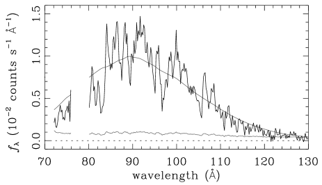
Figure 12: EUVE SW count spectrum accumulated between JD 2450367.2 and 2450372.5. The trace at the bottom of the figure is the $1\,\sigma$ error vector and the smooth curve is an absorbed blackbody model. Exposure time is 75.1 ks, the bin width $\Delta\lambda=0.2$ Å, and the observed SW count rate is 0.28 counts s^-1.

Although Fig. 12 demonstrates that the extreme-ultraviolet spectrum of SS Cyg is not well described by an absorbed blackbody, it is useful to parameterize it in that way in order to obtain an estimate of flux emitted outside of the EUVE bandpass. For the absorption cross section, we used the parameterization of ? for H I, He I and He II with abundance ratios of 1:0.1:0.01, as is typical of the diffuse interstellar medium. We “fitted” the observed spectrum to this model using the SW hardness ratio $H/S$ and a fiducial count rate $H+S=0.5~{}\rm counts~{}s^{-1}$ to constrain $kT$, $N_{\rm H}$, and $f$ assuming $M_{\rm wd}=1~{}\rm M_{\odot}$ (hence $R_{\rm wd}=5.5\times 10^{8}~{}\rm cm$), and $d=100$ pc. The count spectrum of one such model (with $kT=20$ eV, $N_{\rm H}=7.6\times 10^{19}~{}\rm cm^{-2}$, $f=4.5\times 10^{-3}$, and $L_{\rm bb}=2.7\times 10^{33}~{}\rm erg~{}s^{-1}$ for the observed SW count rate $H+S=0.28~{}\rm counts~{}s^{-1}$) is shown by the smooth curve in Fig. 12.

As discussed by ?, it is possible to trade off $kT$ and $N_{\rm H}$ to produce acceptable fits to EUVE spectra of SS Cyg, and Figure 13 shows the parameter contours for $H/S$, $f$, and $L_{\rm bb}$ for $kT=10$–40 eV. A stringent upper bound on the parameter space is set by the observed hardness ratio $H/S\leq$1.5, while a weaker lower bound is set by the interstellar column density, which ? estimated to be $N_{\rm H}\approx 3.5\times 10^{19}~{}\rm cm^{-2}$ based on the curve-of-growth of ultraviolet interstellar absorption lines. ? mooted solutions with $kT=20$ eV and 30 eV for the 1993 EUVE SW spectrum of SS Cyg, ? found that solutions with $kT\approx 20$–25 eV described the ROSAT PSPC spectra, and we find that our Chandra LETG spectrum is consistent with $kT\approx 25$ eV. Consequently, at the peak of the outburst we favour solutions with $kT\approx 20$–25 eV, which Fig. 13 shows require $N_{\rm H}\approx 5.9$–$7.3\times 10^{19}~{}\rm cm^{-2}$ and $L_{\rm bb}\approx 1.7$–$4.3\times 10^{33}\rm\,(d/100\,pc)^{2}\,erg\,s^{-1}$.

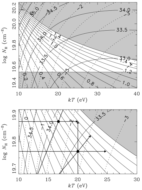
Figure 13: Constraints on the EUVE SW spectrum of SS Cyg. Contours of $H/S$ (solid curves 0.2–1.5), $\log f$ (dotted curves $-4$–1.5), and $\log L_{\rm bb}$ (solid curves 33–36) are plotted as a function of $kT$ and $N_{\rm H}$. The region of parameter space shaded gray is excluded by the conditions $H/S\leq 1.5$ and $N_{\rm H}{\lower 3.22916pt\hbox{ $>$ }\atop\raise 1.50694pt\hbox{ $\sim$}}3.5\times 10^{19}~{}\rm cm^{-2}$. The lower panel shows a detail of the parameter space with five example trajectories of SS Cyg during the course of the 1996 October outburst; the tracks start at the filled circle and move left and/or up, then to the right and/or down.

To investigate the temporal evolution of the extreme-ultraviolet spectrum of SS Cyg during its 1996 October outburst, we show in the lower panel of Fig. 13 five representative trajectories through the ($kT$, $N_{\rm H}$) parameter space. In the first set of examples, $N_{\rm H}$ is assumed to be constant throughout the outburst, so the trajectories follow the horizontal tracks. In the first case, $kT$ starts out at $\approx 20$ eV ($H/S\approx 1.0$) at the beginning of the outburst, rises to $\approx 25$ eV ($H/S\approx 1.3$) at the peak of the outburst, then falls to ${\lower 3.22916pt\hbox{ $<$ }\atop\raise 1.50694pt\hbox{ $\sim$}}17$ eV ($H/S{\lower 3.22916pt\hbox{ $<$ }\atop\raise 1.50694pt\hbox{ $\sim$}}0.8$) at the end of the outburst. In the second case, $kT$ starts out at $\approx 17$ eV at the beginning of the outburst, rises to $\approx 20$ eV at the peak of the outburst, and then falls to ${\lower 3.22916pt\hbox{ $<$ }\atop\raise 1.50694pt\hbox{ $\sim$}}15$ eV at the end of the outburst. In the third example, $kT$ is assumed to be constant at 20 eV throughout the outburst, so the trajectory follows the vertical track. In that case, $N_{\rm H}$ starts out at $\approx 5.9\times 10^{19}~{}\rm cm^{-2}$ at the beginning of the outburst, rises to $\approx 7.3\times 10^{19}~{}\rm cm^{-2}$ at the peak of the outburst, and then falls to ${\lower 3.22916pt\hbox{ $<$ }\atop\raise 1.50694pt\hbox{ $\sim$}}3.4\times 10^{19}~{}\rm cm^{-2}$ at the end of the outburst. In the second set of examples, both $N_{\rm H}$ and $kT$ are assumed to increase during outburst, so the trajectories move along the diagonal tracks in the figure. For the five examples, the parameters at the peak of the outburst are: $kT\approx(17$, 20, 22, 25) eV, $N_{\rm H}\approx(10$, 7.3, 6.6, $5.9)\times 10^{19}~{}\rm cm^{-2}$, $f\approx(53$, 6.9, 3.0, $1.2)\times 10^{-3}$, and $L_{\rm bb}\approx(17$, 4.3, 2.7, $1.7)\times 10^{33}\,\rm(d/100\,pc)^{2}\,erg\,s^{-1}$.

Figs. 3 & 13 show that during the rise to and decline from outburst, the EUVE DS and SW count rate evolution can be driven by variations in $kT$, $N_{\rm H}$, and/or $f$ (hence $L_{\rm bb}$). At one extreme, it is possible that $N_{\rm H}$ is fixed, and that the dramatic increase in the count rates at the beginning of the outburst is caused mostly by an increase in $kT$ from ${\lower 3.22916pt\hbox{ $<$ }\atop\raise 1.50694pt\hbox{ $\sim$}}10$ eV to $\approx 25$ eV. At the other extreme, it is possible that $kT$ is fixed, and that the rapid increase in the count rates at the beginning of the outburst is caused mostly by an increase in $f$, hence $L_{\rm bb}$. These two extreme possibilities imply very different bolometric corrections to convert from the observed SW count rate to luminosity, but unfortunately we do not have the data to determine which applies (however, see Sect. 4.3).

4.2 X-ray spectra

The RXTE PCA provides low-resolution X-ray spectroscopy throughout our observations, allowing us to convert the RXTE count rate to X-ray energy flux. The detailed analysis of the X-ray spectrum is beyond the scope of this paper, and is presented by Wheatley (in preparation). We find that the RXTE spectrum throughout outburst is well represented by a single-temperature thermal-plasma model with the addition of a 6.4 keV line and 8 keV absorption edge ($\chi^{2}$ of 670 with 819 degrees of freedom). Figure 14 shows the best-fitting temperatures and fluxes.

Figure 14: The results of fitting a thermal plasma model to our X-ray spectra of SS Cyg. This model consists of a mekal plasma model, a 6.4 keV emission line, and an 8 keV absorption edge. A full description and motivation is given by Wheatley (2003); the fitted fluxes are discussed in Sect. 4.2. All errors are 68% confidence for one parameter of interest ($\Delta\chi^{2}=1.0$).

Our fitted fluxes provide an estimate of the accretion rate through the boundary layer onto the white dwarf. In contrast to the EUVE band, bolometric corrections are not a serious problem in hard X-rays because the bremsstrahlung spectrum is relatively flat, the RXTE bandpass is so wide, and photoelectric absorption is much less strong.

We are most interested in the accretion rates before the X-ray rise and immediately before the sharp X-ray suppression. The first provides an estimate of the accretion rate in quiescence, the second provides an estimate of the accretion rate at which the boundary layer becomes optically-thick to its own emission. A simple inspection of Fig. 14 shows that the flux after the X-ray recovery (at the end of outburst) is the same as that immediately before the sharp X-ray suppression. We can thus be confident that this represents the maximum luminosity of the optically-thin boundary layer in SS Cyg.

The 3–20 keV fluxes are $\rm 6.1\times 10^{-11}\,erg\,cm^{-2}\,s^{-1}$ (from our first spectrum) and $\rm 20\times 10^{-11}\,erg\,cm^{-2}\,s^{-1}$ (from our third spectrum). Including bolometric corrections of 1.8 to account for flux lost outside our bandpass we find luminosities of $\rm 1.3\times 10^{32}\,(d/100\,pc)^{2}\,erg\,s^{-1}$ and $\rm 4.4\times 10^{32}\,(d/100\,pc)^{2}\,erg\,s^{-1}$, which scale to luminosities of $\rm 3.6\times 10^{32}\,erg\,s^{-1}$ and $\rm 12\times 10^{32}\,erg\,s^{-1}$ using the HST/FGS parallax distance of 166 pc [Harrison et al.¡1999¿]. Using the relation $L=GM_{\rm wd}\dot{M}/2R_{\rm wd}$, and assuming $M_{\rm wd}=1\,\rm M_{\odot}$ (hence $R_{\rm wd}=5.5\times 10^{8}~{}\rm cm$), these luminosities correspond to accretion rates of $\rm 3\times 10^{15}\,g\,s^{-1}$ and $\rm 1\times 10^{16}\,g\,s^{-1}$.

Assuming the flux measured in our first spectrum represents the true quiescent flux, then the derived accretion rates are uncomfortably high for disc-instability models. Predicted accretion rates in quiescence are in the region $\rm 10^{13}\,g\,s^{-1}$ (e.g. ?), two and a half orders of magnitude less than that observed in SS Cyg. This difference has not been satisfactorily explained, and remains one of the main deficiencies of the disc instability model.

In SS Cyg the transition of the boundary layer to its optically-thick state happens at an accretion rate only a factor three above the quiescent rate. This is precisely the rate predicted by ? and ?, though it should be pointed out that these models were developed in response to the discovery of hard X-rays from SS Cyg itself.

4.3 Combination of RXTE and EUVE spectral results

In Sect. 3.1 we point out that the early and late EUVE lightcurve follows the RXTE lightcurve closely, and we conclude that at those times the EUVE count rate is dominated by photons from the soft tail of the hard X-ray emission component. We can test this conclusion by extrapolating our RXTE spectral fits to the EUVE bandpass.

Taking our fitted model for the third RXTE spectrum (Fig. 14) and folding it through the response of the EUVE DS instrument we find a predicted count rate of 0.2 s^-1. Remarkably this is substantially above the measured DS count rate at this time, 0.03 s^-1. To reduce the model-predicted count rate to this level we need to increase the absorption column density from the interstellar value of $N_{\rm H}=3\times 10^{19}\rm\,cm^{-2}$ to $13\times 10^{19}\rm\,cm^{-2}$. This increase is acceptable since the higher absorption still results in negligible absorption in the RXTE bandpass. Assuming the absorption does not vary during outburst, this high $N_{\rm H}$ points to the higher luminosity fits to the EUVE spectrum in Sect. 4.1: around $\rm 10^{35}\,erg\,s^{-1}$ at maximum, corresponding to accretion rates around $\rm 10^{18}\,g\,s^{-1}$ (assuming $M_{\rm wd}=1\,M_{\odot}$ and d=166 pc).

A second constraint on the EUVE spectrum from our RXTE fitting is the boundary layer flux at the time of the transition from dominant X-ray to extreme-ultraviolet emission. Our RXTE fitting shows that the X-ray emission reaches a maximum flux of $\rm 2\times 10^{-10}\,erg\,cm^{-2}\,s^{-1}$. Assuming that the accretion rate continues to rise during this transition, the extreme-ultraviolet spectrum must be capable of radiating at the same rate, but with a measured count rate of just 0.01 s^-1 (see Fig. 2). At $N_{\rm H}=3\times 10^{19}\rm\,cm^{-2}$ this implies a blackbody temperature of just 6 eV. Even with the higher absorption implied by the extrapolation of the RXTE spectrum to the EUVE band ($N_{\rm H}=1.3\times 10^{20}\rm\,cm^{-2}$) the blackbody temperature can rise only to 9 eV. Thus looking again at the possible evolutionary tracks of the extreme-ultraviolet section outlined in Sect. 4.1 and Fig. 13, we find that the blackbody temperature must begin low and increase during the extreme-ultraviolet rise. We can thus rule out spectral evolution in which only the absorption varies.

5 Discussion

5.1 The X-ray delay

For the first time we have resolved the very beginning of the high-energy rise in a dwarf nova outburst. The rise begins in hard X-rays 0.9–1.4 d after the beginning of the rise in the optical, and 0.5 d after the optical brightness crosses $\rm m_{vis}$=11 (which is better defined). The extreme-ultraviolet emission does not begin to rise for another 0.6 d.

We interpret the beginning of the X-ray rise as the moment at which outburst material first reaches the boundary layer. It thus provides a precise measurement of the time the outburst heating wave reaches the boundary layer. Unfortunately the optical observations are not sufficiently evenly spaced to allow us to determine the precise timing of the beginning of the progression of the heating wave, but the propagation time must be in the range 0.9–1.4 d.

The first measurements of a delay between the rise at long and short wavelengths was made with the International Ultraviolet Explorer (e.g. ?), and it has thus been known as the “ultraviolet delay”. However, we believe that the X-ray delay is a better measure of the propagation time of disc heating wave. This is because X-rays are emitted from a precisely known location at the inner edge of the accretion disc, as determined by eclipse studies [Mukai et al.¡1997¿, Wheatley & West¡2003¿].

Target-of-opportunity observations with EUVE have yielded precise rise times for three dwarf novae [Mauche, Mattei & Bateson¡2001¿] and several authors have used these as a measure of the heating wave propagation times (e.g. ?; ?; ?; ?; ?). Our result indicates that the heating wave must propagate even faster than inferred by these authors.

5.2 Boundary layer emission

At the beginning of the high-energy outburst the X-ray emission rises sharply, but with no change in the X-ray spectrum. We take this as evidence that the quiescent and early-outburst X-ray emission arise from the same source, presumably the boundary layer. Furthermore, the precise co-incidence of the timing of the EUV rise and the X-ray suppression shows that the EUV component must also arise in the boundary layer.

Our measured X-ray luminosities (Sect. 4.2) translate to accretion rates of $\rm 3\times 10^{15}\,g\,s^{-1}$ in quiescence and $\rm 1\times 10^{16}\,g\,s^{-1}$ immediately before the boundary layer becomes optically-thick. This quiescent rate is two and a half orders of magnitude higher than that predicted by the standard disc instability model (e.g. ?). Somehow the models need to allow the quiescent disc to transfer more material.

One way to increase the accretion rate of dwarf novae in quiescence is to truncate the accretion disc. Several mechanisms have been proposed including the weak magnetic field of the white dwarf [Livio & Pringle¡1992¿], some kind of heating mechanism leading to disc evaporation [Meyer & Meyer-Hofmeister¡1994¿], and irradiation by the hot white dwarf [King¡1997¿]. ? claim to see the effects of this truncation in the X-ray spectrum of SS Cyg (but see also Wheatley & Mauche, in prep.).

Rather than truly truncating the quiescent accretion disc, the scheme of ? forces in the inner disc to remain in the outburst state permanently. Since material is transferred efficiently in this state, the resulting accretion rate is the same as that of a truncated disc. The calculations of ? suggest that the inner accretion disc can remain in the outburst state through quiescence, even without the need for irradiation. This would naturally explain the high X-ray luminosity of SS Cyg in quiescence.

5.3 Origin of the residual X-ray emission during outburst

Although we are confident that the hard X-ray emission during quiescence and the rise at the beginning of outburst are due to the boundary layer, we are less sure of the origin of the X-ray emission during outburst. This emission has a much lower temperature, which is puzzling if one believes the temperature is set by the depth of the potential well and not the accretion rate. It is also a much smaller fraction of the bolometric luminosity.

? suggest that the outburst emission is due to a density gradient in the outburst boundary layer, such that the upper levels of this region are optically thin. Their Figure 8 shows a schematic in which an optically-thin hard X-ray emitting region sits above the optically-thick extreme-ultraviolet-emitting boundary layer. Their interpretation is attractive because it does not require a second source of the X-rays.

On the other hand, eclipse observations of OY Car do provide evidence for a second source of X-ray emission during outburst. X-ray observations [Naylor et al.¡1988¿, Pratt et al.¡1999a¿] and extreme-ultraviolet [Mauche & Raymond¡2000¿] observations of OY Car in superoutburst show that the X-ray and extreme-ultraviolet emitting regions must be much larger during outburst than in quiescence. ? argue that the EUVE extreme-ultraviolet spectrum of OY Car in superoutburst is due to scattering of optically-thick boundary layer emission in an extended photo-ionised accretion-disc wind. The direct boundary layer emission must by obscured from view, probably by the disc itself.

In contrast, scattering is unlikely to account for the extended source of X-rays in OY Car in superoutburst because of the relative absence of strong resonance lines in the X-ray band. Any scattered component must therefore be much weaker even than the direct flux visible in low-inclination systems such as SS Cyg. ROSAT observations, however, show that OY Car is actually brighter in outburst than quiescence. ? find a ROSAT HRI count rate of 0.016 s^-1 in quiescence and ? find an outburst count rate of 0.028 s^-1 (note that the quiescent count rates in their Table 1 refer to the PSPC detector). We conclude that the relative brightness of the outburst X-ray emission of OY Car points to a second source of X-ray emission that must be inherently larger than the boundary layer.

A candidate is a magnetically-heated accretion-disc corona. This is plausible because the accretion disc is believed to be more magnetically active in outburst than in quiescence, and indeed it is a magneto-rotational instability that is believed to drive the enhanced effective viscosity during outburst [Balbus & Hawley¡1991¿].

6 Conclusions

In this paper we present simultaneous optical, extreme-ultraviolet and X-ray observations of SS Cyg throughout outburst. For the first time we resolve the beginning of the high-energy outburst, which starts in the hard X-ray band 0.9–1.4 d after the beginning of the optical rise (Sect. 3.1). The X-ray rise continues for 0.6 d with the luminosity increasing from $\rm 3.6\times 10^{32}\,erg\,s^{-1}$ to $\rm 1.2\times 10^{33}\,erg\,s^{-1}$. The implied accretion rate in quiescence is two and a half orders of magnitude higher than predicted by the standard disc instability model, and this remains one of the main deficiencies of that model (Sects. 4.2 & 5.2). This discrepancy may be resolved if one allows the inner accretion disc to remain in the outburst state throughout quiescence (e.g. ?). After 0.6 d the X-ray flux drops to near zero in less than three hours, and is replaced immediately with extreme-ultraviolet emission. This is the first time this transition has been resolved, and the coincidence of the X-ray fall and extreme-ultraviolet rise leaves no doubt that both components originate in the boundary layer between accretion disc and white dwarf. The boundary layer may also account for the residual hard X-ray emission in quiescence, but we argue that some form of magnetic heating of a disc corona is more likely (Sect. 5.3).

The X-ray rise defines the moment at which outburst material first reaches the boundary layer, and so authors who have used the extreme-ultraviolet rise to infer the propagation time of the outburst heating wave may have over-estimated the propagation time by 0.6 d in SS Cyg (Sect. 5.1).

The extreme-ultraviolet band dominates during most of the outburst, peaking at a luminosity around $\rm 5\times 10^{34}\,erg\,s^{-1}$ (Sects. 4.1 & 4.3). Dwarf nova oscillations are seen with high amplitude throughout the extreme-ultraviolet outburst, but are not present in our X-ray lightcurves. This suggests that the source of the oscillations operates only in the optically-thick boundary layer, though it is also possible that the X-ray oscillations are smeared out by a long X-ray cooling timescale (Sect. 3.4).

At the end of outburst the boundary layer emission switches back to the X-ray band, this time more slowly, but at the same luminosity/accretion rate as before (Fig. 14). The instrumental count rates clearly depend strongly on the changing spectrum during these transitions, and the X-ray hardness ratio appears to be the best indicator of the accretion rate at these times (Sect. 3.2.2). The transitions between X-ray and extreme-ultraviolet emission are accompanied by intense variability, that (sometimes at least) takes the form of quasi-periodic oscillations with periods around 200 s (Sect. 3.3). These variations are not associated with hardness variations and by inferring that the X-ray cooling timescale must be shorter than these variations we were able to limit the density of the X-ray emitting plasma to be greater than $5\times 10^{13}\,\rm cm^{-3}$ (Sect. 3.3.1).

References

- [Abbott et al.¡1996¿] Abbott, M. J., Boyd, W. T., Jelinsky, P., Christian, C., Miller-Bagwell, A., Lampton, M., Malina, R. F. & Vallerga, J. V., 1996, ApJS, 107, 451.
- [Balbus & Hawley¡1991¿] Balbus, S. A. & Hawley, J. F., 1991, ApJ, 376, 214.
- [Bath & Pringle¡1982¿] Bath, G. T. & Pringle, J. E., 1982, MNRAS, 199, 267.
- [Bowyer & Malina¡1991¿] Bowyer, S. & Malina, R. F., 1991, In: Extreme Ultraviolet Astronomy, 397, eds Malina, R. F. & Bowyer, S., New York: Pergamon.
- [Bowyer et al.¡1994¿] Bowyer, S. et al., 1994, ApJS, 93, 569.
- [Cannizzo & Mattei¡1992¿] Cannizzo, J. K. & Mattei, J. A., 1992, ApJ, 401, 642.
- [Cannizzo & Mattei¡1998¿] Cannizzo, J. K. & Mattei, J. A., 1998, ApJ, 505, 344.
- [Cannizzo¡1993¿] Cannizzo, J. K. In: ed. Wheeler, J. C., Accretion Disks in Compact Stellar Systems, 6, World Scientific, Singapore, 1993.
- [Cannizzo¡2001¿] Cannizzo, J. K., 2001, ApJ, 556, 847.
- [Done & Osborne¡1997¿] Done, C. & Osborne, J. P., 1997, MNRAS, 288, 649.
- [Hameury, Lasota & Dubus¡1999¿] Hameury, J., Lasota, J. & Dubus, G., 1999, MNRAS, 303, 39.
- [Hameury, Lasota & Warner¡2000¿] Hameury, J., Lasota, J. & Warner, B., 2000, A&A, 353, 244.
- [Harrison et al.¡1999¿] Harrison, T. E., McNamara, B. J., Szkody, P., McArthur, B. E., Benedict, G. F., Klemola, A. R. & Gilliland, R. L., 1999, ApJ, 515, L93.
- [Hassall et al.¡1983¿] Hassall, B. J. M., Pringle, J. E., Schwarzenberg-Czerny, A., Wade, R. A., Whelan, J. A. J. & Hill, P. W., 1983, MNRAS, 203, 865.
- [Jones & Watson¡1992¿] Jones, M. H. & Watson, M. G., 1992, MNRAS, 257, 633.
- [King¡1997¿] King, A. R., 1997, MNRAS, 288, L16.
- [Lasota¡2001¿] Lasota, J. P., 2001, New Astron. Rev., 45, 449.
- [Livio & Pringle¡1992¿] Livio, M. & Pringle, J. E., 1992, MNRAS, 259, L23.
- [Long et al.¡1996¿] Long, K. S., Mauche, C. W., Raymond, J. C., Szkody, P. & Mattei, J. A., 1996, ApJ, 469, 841.
- [Mason et al.¡1978¿] Mason, K. O., Lampton, M., Charles, P. & Bowyer, S., 1978, ApJ, 226, 129.
- [Mason et al.¡1988¿] Mason, K. O., Córdova, F., Watson, M. G. & King, A. R., 1988, MNRAS, 232, 779.
- [Mattei, Saladyga & Waagen¡1985¿] Mattei, J. A., Saladyga, M. & Waagen, E. O., 1985, SS Cygni light curves 1896-1985, AAVSO Monograph, Cambridge: American Association of Variable Star Observers (AAVSO), —c1985, edited by Mattei, Janet A.; Saladyga, Michael; Waagen, Elizabeth O.
- [Mattei¡1996a¿] Mattei, J. A., 1996a, AAVSO Alert Notice, 221.
- [Mattei¡1996b¿] Mattei, J. A., 1996b, AAVSO Alert Notice, 222.
- [Mattei¡1996c¿] Mattei, J. A., 1996c, AAVSO Alert Notice, 229.
- [Mauche & Raymond¡2000¿] Mauche, C. W. & Raymond, J. C., 2000, ApJ, 541, 924.
- [Mauche & Robinson¡2001¿] Mauche, C. W. & Robinson, E. L., 2001, ApJ, 562, 508.
- [Mauche, Mattei & Bateson¡2001¿] Mauche, C. W., Mattei, J. A. & Bateson, F. M., 2001, In: ASP Conf. Ser. 229: Evolution of Binary and Multiple Star Systems, 367, eds Podsiadlowski, P., Rappaport, S., King, A. R., D’Antona, F. & Burder, L., ASP, San Francisco.
- [Mauche, Raymond & Córdova¡1988¿] Mauche, C. W., Raymond, J. C. & Córdova, F. A., 1988, ApJ, 335, 829.
- [Mauche, Raymond & Mattei¡1995¿] Mauche, C. W., Raymond, J. C. & Mattei, J. A., 1995, ApJ, 446, 842.
- [Mauche¡1996¿] Mauche, C. W., 1996, In: ASSL Vol. 208: IAU Colloq. 158: Cataclysmic Variables and Related Objects, 243, eds Evans, A. & Wood, J. H., Kluwer, Dordrecht.
- [Meyer & Meyer-Hofmeister¡1981¿] Meyer, F. & Meyer-Hofmeister, E., 1981, A&A, 104, L10.
- [Meyer & Meyer-Hofmeister¡1994¿] Meyer, F. & Meyer-Hofmeister, E., 1994, A&A, 288, 175.
- [Mukai et al.¡1997¿] Mukai, K., Wood, J. H., Naylor, T., Schlegel, E. M. & Swank, J. H., 1997, ApJ, 475, 812.
- [Mukai et al.¡2003¿] Mukai, K., Kinkhabwala, A., Peterson, J. R., Kahn, S. M. & Paerels, F., 2003, ApJ, 586, L77.
- [Naylor et al.¡1988¿] Naylor, T., Bath, G. T., Charles, P. A., Hassall, B. J. M., Sonneborn, G., van der Woerd, H. & van Paradijs, J., 1988, MNRAS, 231, 237.
- [Osaki¡1974¿] Osaki, Y., 1974, PASP, 26, 429.
- [Osaki¡1996¿] Osaki, Y., 1996, PASP, 108, 39.
- [Patterson & Raymond¡1985¿] Patterson, J. & Raymond, J. C., 1985, ApJ, 292, 535.
- [Pickering & Fleming¡1896¿] Pickering, E. C. & Fleming, W., 1896, ApJ, 4, 369.
- [Ponman et al.¡1995¿] Ponman, T. J., Belloni, T., Duck, S. R., Verbunt, F., Watson, M. G. & Wheatley, P. J., 1995, MNRAS, 276, 495.
- [Pratt et al.¡1999a¿] Pratt, G. W., Hassall, B. J. M., Naylor, T., Wood, J. H. & Patterson, J., 1999a, MNRAS, 309, 847.
- [Pratt et al.¡1999b¿] Pratt, G. W., Hassall, B. J. M., Naylor, T. & Wood, J. H., 1999b, MNRAS, 307, 413.
- [Press et al.¡1992¿] Press, W. H., Teulolsky, S. A., Vetterling, W. T. & Flannery, B. P., 1992, Numerical recipes: The art of scientific computing, Cambridge University Press, Second edition.
- [Pringle & Savonije¡1979¿] Pringle, J. E. & Savonije, G. J., 1979, MNRAS, 187, 777.
- [Pringle et al.¡1987¿] Pringle, J. E., Bateson, F. M., Hassall, B. J. M., Heise, J., Van der Woerd, H., Holberg, J. B., Polidan, R. S., Van Amerongen, S., Van Paradijs, J. & Verbunt, F., 1987, MNRAS, 225, 73.
- [Ricketts, King & Raine¡1979¿] Ricketts, M. J., King, A. R. & Raine, D. J., 1979, MNRAS, 186, 233.
- [Rumph, Bowyer & Vennes¡1994¿] Rumph, T., Bowyer, S. & Vennes, S., 1994, AJ, 107, 2108.
- [Smak¡1984¿] Smak, J., 1984, PASP, 96, 5.
- [Smak¡1998¿] Smak, J. I., 1998, Acta Astronomica, 48, 677.
- [Stehle & King¡1999¿] Stehle, R. & King, A. R., 1999, MNRAS, 304, 698.
- [Swank et al.¡1978¿] Swank, J. H., Boldt, E. A., Holt, S. S., Rothschild, R. E. & Serlemitsos, P. J., 1978, ApJ, 226, L133.
- [Swank¡1979¿] Swank, J. H., 1979, In: White dwarfs and variable degenerate stars, 135, eds Van Horn, H. M. & Weidemann, V., Rochester University Press.
- [Truss et al.¡2000¿] Truss, M. R., Murray, J. R., Wynn, G. A. & Edgar, R. G., 2000, MNRAS, 319, 467.
- [Verbunt, Wheatley & Mattei¡1999¿] Verbunt, F., Wheatley, P. J. & Mattei, J. A., 1999, A&A, 346, 146.
- [Verner, Verner & Ferland¡1996¿] Verner, D. A., Verner, E. M. & Ferland, G. J., 1996, Atomic Data and Nuclear Data Tables, 64, 1.
- [Wheatley & West¡2003¿] Wheatley, P. J. & West, R. G., 2003, MNRAS, submitted.
- [Wheatley et al.¡1996a¿] Wheatley, P. J., Van Teeseling, A., Watson, M. G., Verbunt, F. & Pfeffermann, E., 1996a, MNRAS, 283, 101.
- [Wheatley et al.¡1996b¿] Wheatley, P. J., Verbunt, F., Belloni, T., Watson, M. G., Naylor, T. & Ishida, M., 1996b, A&A, 307, 137.