Branch, Spur, and Feather Formation in Spiral Galaxies

Abstract

We use hydrodynamical simulations to investigate the response of geometrically thin, self-gravitating, singular isothermal disks of gas to imposed rigidly rotating spiral potentials. By minimizing reflection-induced feedback from boundaries, and by restricting our attention to models where the swing parameter $X\sim 10$, we minimize the swing amplification of global normal modes even in models where Toomre’s $Q_{g}\sim 1-2$ in the gas disk. We perform two classes of simulations: short-term ones over a few galactic revolutions where the background spiral forcing is large, and long-term ones over many galactic revolutions where the spiral forcing is considerably smaller. In both classes of simulations, the initial response of the gas disk is smooth and mimics the driving spiral field. At late times, many of the models evince substructure akin to the so-called branches, spurs, and feathers observed in real spiral galaxies. We comment on the parts played respectively by ultraharmonic resonances, reflection off internal features produced by nonlinear dredging, and local, transient, gravitational instabilites within spiral arms in the generation of such features. Our simulations reinforce the idea that spiral structure in the gaseous component becomes increasingly flocculent and disordered with the passage of time, even when the background population of old disk stars is a grand-design spiral. We speculate that truly chaotic behavior arises when many overlapping ultraharmonic resonances develop in reaction to an imposed spiral forcing that has itself a nonlinear, yet smooth, wave profile.

1 Introduction

Nearly all spiral galaxies, even the grand designs in blue light, display intricate features superimposed on the main spiral arms. Unruly branches, spurs, and feathers invariably lend a ragged appearance to the overall spiral structure. Roberts (1969) showed that two-armed galactic shocks can arise from the nonlinear response of the gas to an ordered and steady spiral potential associated with a background of disk stars. Shu, Milione, & Roberts (1973, hereafter SMR) demonstrated that additional prominent, azimuthally nonsinusoidal, features could appear as a consequence of ultraharmonic resonances with the two-armed driving potential, and they suggested that self-gravity, not included in their formal calculations, may enhance the intrinsically nonlinear response of the gas. Their suggestion is particularly attractive after the discovery that many spiral galaxies possess grand-design spirals in infrared light despite looking quite flocculent in their gas distributions and Population I stars (Block & Wainscoat 1991; Block et al. 1994; Block, Elmegreen, & Wainscoat 1996). Block & coworkers, however, give a quite different interpretation to their findings, and we shall return in § 7 to contrast their views with ours.

Woodward (1975) carried out one-dimensional time-dependent numerical calculations which studied the azimuthal flow of gas in both steady as well as time-varying spiral potentials. He did not include the self-gravity the gas, and he found only the strongest (4:1) ultraharmonic resonance discussed by SMR. Moreover, he found that numerical viscosity inhibited the development of secondary shocks. Woodward concluded that unless self-gravity of the gas is significant, spiral substructure could not be explained in terms of ultraharmonic resonances. Fortunately, gravitation is universal, and the self-gravity of the cold component of the interstellar gas cannot be ignored in real disk galaxies on the scale of the spiral arms.

Given the dissipative nature of interstellar gas, it is natural to associate some of the fragmented features in the overall spiral structure with corotating but sheared disturbances that arise from local gravitational instability (Goldreich & Lynden-Bell 1965) or as a steady response to an imposed point mass (Julian & Toomre 1966). Piddington (1973) noted that feathers and spurs are often seen in combination, as if they are manifestations of a single phenomenon. By examining the pitch angles and widths of spurs and feathers in conjunction with kinematic arguments, Elmegreen (1980) argued that they can be identified as density waves. The detailed analysis of the morphology of NGC 1566 by Elmegreen & Elmegreen (1990) led to the association of several optical features with resonances, including two ultraharmonic resonances (see also Visser’s 1980 use of SMR’s code to identify the long spiral branches seen between the main spiral arms of M81 with the 4:1 ultraharmonic resonance). Thus, the substructure that we observe in real galaxies may be a hybrid phenomenon, i.e., a mixture of the transient swing-amplification of “shearing bits and pieces” (Toomre 1981, 1990, 1991), especially near the corotation circle, and nonlinear structures produced by the processes discussed in this paper.

Balbus & Cowie (1985) studied the transient gravitational instability of local quasi-axisymmetric disturbances in the linear regime, but against a background of nonlinear flow represented by the Robert’s (1969) shock solutions for the steady (non-self-gravitating) response of gas to the forcing of a background spiral potential. (The linear studies of Goldreich & Lynden-Bell 1965 and Julian & Toomre 1966 have base states that are time-independent and axisymmetric.) Balbus & Cowie considered the expanding shear flow as the gas leaves an arm region well-displaced from the corotation circle (another difference with the earlier studies), and they proposed a simple modification of Toomre’s (1964) $Q_{g}\rightarrow Q_{\rm sp}$ criterion as applied to gas disks to characterize the onset of local Jeans instability behind spiral arms. We return to this modified value of $Q_{\rm sp}$ in our discussion of feathers in § 7.

Balbus (1988) extended the study by investigating all wavenumber directions in the disk plane, and discovered two preferred directions for initial wavenumbers for the temporary growth of gravitational instabilities: roughly parallel and perpendicular to the main spiral arm. He suggested that periodic, closely spaced, spurs may develop in the former, while the latter favors nonperiodic spur formation. We shall henceforth use the name “feathers” for both types of features produced by local gravitational instability of a transient kind. We reserve the name “spurs” for distinctly leading spiral features, which do not form by this mechanism according to our interpretation. These spurs protrude from the main arms and have shorter azimuthal extent than the “branches”, which in our interpretation are due to the ultraharmonic resonances.

Kim & Ostriker (2002, hereafter KO) carried out local magnetohydrodynamic (MHD) simulations and found that magnetic fields are crucial for the formation of feathers (called by them as “spurs”) when the Toomre $Q_{g}$ parameter for the gas is not small. The magneto-Jeans instability arises more easily than the purely hydrodynamic calculations (for which the $Q_{\rm sp}$ criterion works reasonably well) because magnetic fields destroy the stabilizing effects of potential-vorticity conservation behind galactic shocks (see also Lynden-Bell 1966 and Elmegreen 1993). The net result is to form a wing of feathers that jut out individually, more-or-less perpendicularly, on the downstream side of the shock front at the main spiral arms.

In this paper, we carry out two-dimensional, global, hydrodynamic simulations that incorporate the self-gravity of the gas. We work within the context of the singular isothermal disk (SID) to understand the dynamical formation of spiral substructure in self-gravitating, purely hydrodynamical systems. However, in our physical interpretations, we shall identify the formation of feathers in low Toomre-$Q_{g}$ systems as the equivalent (inside spiral arms) of an MHD system with high effective $Q_{g}$ values. This is important because we shall find that low $Q_{g}$ gas-disks with relatively high forcing cannot be evolved for many galactic rotations in hydrodynamic simulations without developing catastrophic increases in the surface density in many regions. In high $Q_{g}$ disks, we can carry the hydrodynamic simulations forward for the much longer times that are necessary to accumulate resonant influences and to see the side-effects of nonlinear dredging. The result is a much richer variety of nonlinear substructure, including spurs and hints of chaotic behavior akin to flocculence – but no feathers. Thus, we speculate that more complete, whole-disk, MHD simulations of moderately high effective $Q_{g}$ gas disks will find branches, spurs, and feathers as possible substructures within a single self-consistent simulation, with flocculence a possible end-product if the system becomes chaotic through the effects of overlapping ultraharmonic resonances.

The dynamics of SIDs, with their self-similar surface density ($\Sigma\propto 1/\varpi$) and flat rotation curves ($v_{\rm rot}={\rm constant}$) have been intensively studied in the forty years following Mestel’s (1963) groundbreaking article. They are reasonable analogs for disk galaxies, while their self-similarity and overall simplicity lend them to detailed analytic and semi-analytic investigations. The properties of SIDs in the context of spiral galaxies have been reviewed and explored by Shu et al (2000, hereafter S00), who studied their linear stability properties, both in the context of their susceptibility to nonaxisymmetric bifurcations, as well as their ability to promote swing over-reflection of wave trains impinging on the corotation circle. In the current work, we extend the S00 analysis to investigate the nonlinear response of gaseous SID structures to spiral gravitational perturbations arising from an imposed rigidly rotating spiral pattern present in the stellar component of a disk galaxy.

2 Partial SIDs

A massive spiral disturbance sliding through unperturbed gas is bound to cause complicated unrest. Numerical simulations are thus an ideal tool for investigating the nonlinear response of a self-gravitating, differentially rotating, razor-thin, gas disk to a steady spiral forcing potential. The simulations presented here adopt a so-called partial SID as the equilibrium reference state. We define the partial fraction of the disk, $F$, as the amount of mass in the gas disk, with the remainder, $1-F$, approximated as a rigid stellar component. Our imposed two-armed trailing-spiral potential, rotating uniformly at a pattern angular speed $\Omega_{p}$, can be thought of as arising from this stellar component. Therefore, in our gas-dynamical models, the stellar disk manifests itself both through a time-independent, axisymmetric, gravitational field, and through the non-axisymmetric perturbing potential. One is equally free to imagine that the radial gravitational field arises from the more realistic combination of a true stellar disk and a nonreactive, spherically symmetric, dark-matter halo, whereas the spiral forcing arises from a normal-mode structure endemic to the true stellar disk. In the latter, more realistic, scenario, the spiral forcing may have relatively small amplitude relative to the total axisymmetric, radial gravitational field, and yet represent a nonlinear perturbation in the infrared surface brightness of the true stellar disk. Thus, we are motivated to consider both linear and nonlinear wave profiles for the planform of the spiral force field.

2.1 Basic Equations

In polar coordinates $(\varpi,\phi)$ and time $t$, we denote the mass per unit area of the gas and stellar components of a completely flattened distribution of matter as $\Sigma_{g}(\varpi,\phi,t)$ and $\Sigma_{*}(\varpi,\phi,t)$ respectively. We model both as isothermal fluids, with the constant stellar dispersive speed being $c_{*}$ and the gaseous isothermal sound speed being $c_{g}$. We denote $u$ and $j$ with the appropriate subscripts as the $\varpi$ component of the fluid velocity and the $z$ component of the specific angular momentum. With these definitions, the equations of continuity and momentum for the gas are written

$$\partial\Sigma_{g}/\partial t+\frac{1}{\varpi}\frac{\partial(\varpi\Sigma_{g}{u_{g}})}{\partial\varpi}+\frac{1}{\varpi^{2}}\frac{\partial(\Sigma_{g}j_{g})}{\partial\phi}=0\,,$$ (1)

$$\partial u_{g}/\partial t+u_{g}\frac{\partial u_{g}}{\partial\varpi}+\frac{j_{g}}{\varpi^{2}}\frac{\partial u_{g}}{\partial\phi}-\frac{j_{g}^{2}}{\varpi^{3}}=-\frac{c_{g}^{2}}{\Sigma_{g}}\frac{\partial\Sigma_{g}}{\partial\varpi}-\frac{\partial{\cal V}}{\partial\varpi}\,,$$ (2)

$$\partial j_{g}/\partial t+u_{g}\frac{\partial j_{g}}{\partial\varpi}+\frac{j_{g}}{\varpi^{2}}\frac{\partial j_{g}}{\partial\phi}=-\frac{c_{g}^{2}}{\Sigma_{g}}\frac{\partial\Sigma_{g}}{\partial\phi}-\frac{\partial{\cal V}}{\partial\phi}\,.$$ (3)

A similar set holds for the disk of stars if we were to allow them actively to respond to the collective gravitational field. For the purposes of the present paper, however, we consider both the axisymmetric and spiral distributions of the stellar component to be rigidly given by external considerations.

In equation (4), ${\cal V}$ is the combined gravitational potential of the gas and the stellar component. It is given by Poisson’s integral:

$${\cal V}(\varpi,\phi,t)=-G\oint d\psi\int_{0}^{\infty}\frac{\Sigma(r,\psi,t)\,rdr}{[r^{2}+\varpi^{2}-2r\varpi\cos(\psi-\phi)]^{1/2}}\,,$$ (4)

where $\Sigma(r,\psi,t)$ is the sum of the gaseous and stellar surface densities at the source point in the disk.

According to S00, the surface density, rotation angular velocity, and epicyclic frequency, of a full, single component, axisymmetric SID have the following properties:

$$\Sigma=\frac{c^{2}}{2\pi G\varpi}(1+D^{2})\,,$$ (5)

$$\Omega=\frac{cD}{\varpi}\,,$$ (6)

$$\kappa=\sqrt{2}\frac{cD}{\varpi}\,,$$ (7)

where $c$ is a dispersive velocity or isothermal sound speed, and $D$ is a dimensionless rotation parameter. S00’s formalism is easily extended to two partial disks in which we attribute the fraction $(1-F)$ of the full gravity in the axisymmetric state to a rigid stellar component and another fraction $F$ to an active gaseous disk:

$$\Sigma_{*}=\frac{(1-F)c^{2}(1+D^{2})}{2\pi G\varpi},\qquad\Sigma_{g}=\frac{Fc^{2}(1+D^{2})}{2\pi G\varpi}.$$ (8)

The coefficients in the above relations are chosen so that the surface density (and gravitational field) remains the same as for the full disk in equation (5).

We denote the angular velocity of the stars and gas, respectively, by $\Omega_{*}=cD_{*}/\varpi$ and $\Omega_{g}=cD_{g}/\varpi$, with associated epicyclic frequencies that are $\surd 2$ larger. Then radial force balance for the stellar and gas disks in their equilibrium states can be expressed by

$$c_{*}^{2}+c^{2}D_{*}^{2}=c_{g}^{2}+c^{2}D_{g}^{2}=c^{2}(1+D^{2}).$$ (9)

Since the full disk has no independent meaning, we are free to choose $c\equiv c_{*}$ and $D\equiv D_{*}$. Expressing $c_{g}$ as a fraction $f$ of $c_{*}$ now, we get from the above, with $c_{g}=fc_{*}$, that

$$D_{g}^{2}=1+D_{*}^{2}-f^{2}.$$ (10)

Since the rotation and epicyclic frequencies of the gas disk are $\Omega_{g}=c_{*}D_{g}/{\varpi}$ and $\kappa_{g}=\sqrt{2}\Omega_{g}$, Toomre’s (1964) axisymmetric-stability parameter, $Q_{g}$ for the gas becomes

$$Q_{g}\equiv\frac{\kappa_{g}c_{g}}{\pi G\Sigma_{g}}=Q_{*}(D_{g}/D_{*})\frac{(1-F)f}{F}\,,$$ (11)

whereas the corresponding value for the dynamically inactive $(1-F)$ fraction of the disk reads,

$$Q_{*}\equiv\frac{\kappa_{*}c_{*}}{\pi G\Sigma_{*}}=2\sqrt{2}\frac{D_{*}}{(1-F)(1+D_{*}^{2})}\,.$$ (12)

For comparison, the full disk has an associated $Q$:

$$Q=2\sqrt{2}\frac{D_{*}}{1+D_{*}^{2}}.$$ (13)

Thus, for a full SID, $Q$ reaches a maximum of $\sqrt{2}$ at a model $D_{*}=1$ and decreases on either side to unity for models where $D_{*}=\sqrt{2}\pm 1$. These values of $D_{*}$ do not corrrespond to very rapidly rotating fiducial systems, so one might think Toomre’s asymptotic stability analysis that depends on $D_{*}\gg 1$ might be called into question. The situation can be partially saved by invoking a rigid massive dark-matter halo to provide some of the radial gravity attributed above to a flat disk of stars. But it also turns out that an exact stability analysis, even for a full disk, yields remarkable agreement with the Toomre criterion, insofar as its predictions concerning fragmentation into rings go (see S00). On the other hand, overall radial collapse occurs in a fundamental way because a disk rotates too slowly (small $D_{*}$), so it cannot be well described by looking only at the $Q$ parameter. In § 2.2 therefore, we re-examine the question of the radial collapse of a partial gas disk from the formal perspective of an exact stability analysis (but keeping the “stellar” disk fixed).

In any case, $Q_{g}$ yields an accurate measure of the response of the active gas to less-than-galactic scale perturbations, whether axisymmetric or nonaxisymmetric. Since the partial gas disk derives much of its support from the rigid stellar component (which can include here a massive dark-matter halo), its $Q_{g}$ surpasses that of the full disk unless $f$ is too small or $F$ is too close to unity. Indeed, it is well known that the addition of a such a rigid component or halo will serve to stabilize the response of the active component of a disk (e.g. Ostriker & Peebles 1973). Increasing the fraction of support from the rigid halo also increases the ratio

$$X={2\over{m}}{D_{g}^{2}\over{F(1+D_{*}^{2})}}\,,$$ (14)

of the azimuthal wavelength to the critical wavelength at which ring fragmentation first occurs. For $X>3$, the swing amplification mechanism (Toomre 1981) loses its effectiveness. In the partial-disk evolutionary simulations presented in this paper, we adopt $F=0.1$, leading to values of the swing parameter $X\sim 10$. The swing amplification of corotating disturbances is therefore effectively minimized in our simulation models.

2.2 Stability of Partial Disk

The Toomre-$Q$ values for a full (as given by equation 13) and a partial SID (as given by equation 11) as functions of $D_{\star}$ are depicted in Figure 1. The full and partial SIDs shown in this figure correspond, respectively, to $F=f=1$ and $F=f=0.1$. Note that since the Q-values for SIDs (both full and partial) are constrained by the rotation parameter $D_{\star}$, it is not possible to get arbitrarily large values for $Q$.

As we have already remarked, Toomre’s stability analysis gives only asymptotically accurate results for a single active component. For completeness, we repeat the exact analysis of S00 for a partial disk when it is the only active component in the system. The more complex, linear stability analysis needed when both the gas and star disks are active has been treated by Lou & Shen (2003). We refer the interested reader to their paper for details.

When an active gas disk is perturbed by a small disturbance, we can linearize the fluid equations (1) - (3) around the basic underlying state. We can then look for perturbation solutions that are periodic in $t$ and $\phi$, e.g.

$$\Sigma_{1}=S(\varpi)e^{im(\omega t-m\varphi)}\,,$$ (15)

and similarly for $u_{1}$, $j_{1}$, and ${\cal V}_{1}$. The pattern speed of the disturbance is given by $\Omega_{p}=\omega/m$. Upon substituting these trial solutions into the linearized fluid equations, and eliminating $u_{1}$ and $j_{1}$, one arrives at a second-order integro-differential equation which describes a global, self-consistent, self-gravitating, spiral density perturbation of the disk (Lin & Lau 1979):

$$(\omega-m\Omega)S+{1\over\varpi}{d\over d\varpi}\left\{{\varpi\Sigma_{g}\over(\omega-m\Omega)^{2}-\kappa^{2}}\left[-2\Omega{m\over\varpi}+(\omega-m\Omega){d\over d\varpi}\right]\Phi\right\}$$

$$-{m\Sigma_{0}\over\varpi[(\omega-m\Omega)^{2}-\kappa^{2}]}\left[(\omega-m\Omega){m\over\varpi}-{\kappa^{2}\over 2\Omega}{d\over d\varpi}\right]\Phi=0.$$ (16)

If we set $\omega=0$ in order to find the marginal conditions for the swing over-reflection of spiral density waves when $m\neq 0$, or for axisymmetric collapse and fragmentation into rings when $m=0$ (see S00), substitution of the reference state values for the partial SID for the surface density, angular and epicyclic frequencies into the above equation leads to:

$$\left[-S+{F\over{D_{g}^{2}(m^{2}-2)}}\left({m^{2}\over{\varpi}}-2{d\over{d\varpi}}-\varpi{d^{2}\over{d\varpi^{2}}}\right)\left({f^{2}\varpi\over{F}}S+{(D_{g}^{2}+f^{2})\over{2\pi G}}V\right)\right]=0\,$$ (17)

where $V$ and $S$ are related through the linearized version of Poisson’s equation

$$V(\varpi)=-G\oint d\chi\int_{0}^{\infty}{S(r)\cos(m\chi)\,rdr\over[r^{2}+\varpi^{2}-2r\varpi\cos\chi]^{1/2}}.$$ (18)

The above two equations admit scale-free solutions of the form (Syer & Tremaine 1996, Lynden-Bell & Lemos 1993)

$$S(\varpi)=s\varpi^{-3/2}e^{i\alpha\ln\varpi}\,$$ (19)

$$V(\varpi)=v\varpi^{-1/2}e^{i\alpha\ln\varpi}\,$$ (20)

with $s$, $v$, and $\alpha$ equal to constants. The pitch angle $i$ of such logarithmic spirals is a constant and given by the formula $\tan i=m/\alpha$. While the perturbation solutions are scale free, they have radial amplitudes which decline more rapidly with $\varpi$ than the underlying equilibrium. Hence, all but infinitesimally small disturbances of the form given by equations (19) and (20) will achieve arbitrary amplitudes sufficiently near the origin, leading to a formal breakdown of the perturbative analysis. This breakdown is generally averted by cutting out a hole in the center of the disk to represent an inactive central bulge (Zang 1976, Evans & Read 1998).

Substituting the scale-free solutions into equations (17) and (18), we obtain the conditions of marginal stability from the solutions of

$$-1+{1\over{D_{g}^{2}(m^{2}-2)}}\left(m^{2}+\alpha^{2}+{1\over{4}}\right)\left(f^{2}-F(f^{2}+D_{g}^{2}){\cal N}_{m}(\alpha)\right)=0\ \,.$$ (21)

Rearranging, we find

$$D_{g}^{2}={(m^{2}+\alpha^{2}+{1\over{4}})(Ff^{2}{\cal N}_{m}(\alpha)-1)\over{2-m^{2}-(m^{2}+\alpha^{2}+{1\over{4}})F{\cal N}_{m}(\alpha)}}\,,$$ (22)

where ${\cal N}_{m}(\alpha)$ is the Kalnajs (1971) proportionality relation for the logarithmic spiral potential-density pairs:

$$v=-2\pi G{\cal N}_{m}(\alpha)s\,,$$ (23)

with

$${\cal N}_{m}={1\over{2}}{\Gamma[(m+1/2+i\alpha)/2]\Gamma[(m+1/2-i\alpha)/2]\over{\Gamma[(m+3/2+i\alpha)/2]\Gamma[(m+3/2-i\alpha)/2]}}\,.$$ (24)

The curves of marginal axisymmetric stability are then calculated by setting $m=0$, and choosing values for $f$ and $F$. Figure 2a shows cases where $F=f$, in increments of 0.1 from $F=f=0.1$ to $F=f=0.9$. For reference, the full disk branches with $F=f=1.0$ are also shown. As the stellar and dark-matter components of the potential become increasingly dominant within the sequence of partial SIDs, the axisymmetric collapse branch disappears rapidly. Thus, we only have to worry about the fragmentation branch for all practical purposes, and the condition of marginal stability for that branch is quite accurately approximated by Toomre’s $Q_{g}$ criterion because increasingly wavy planforms are required to trigger such instabilities in low $F$ systems. We also show the self-consistency curves in Figure 2b for $m=2$ disturbances in increments of 0.1 from $F=f=0.1$ to $F=f=1.0$. Our high $Q_{g}$ disks (with associated rotation parameters cited in § 5) will not support zero frequency spiral waves of any $\alpha$. However, our low $Q_{g}$ disks will support $m=2$ disturbances in the range of $\alpha=0-2$. As described in § 3, we consider two types of spiral planforms in our simulations, namely, the linear logarithmic spiral planform, and the nonlinear SYL planform. The logarithmic spiral planform has associated $\alpha=6.15$, which lies outside the range that would be swing amplified even if it were to propagate into the central regions undamped with similar wavenumber. However, since the SYL planform does have contributions from wavenumbers in the range of $\alpha=0-2$, these wavenumbers could have been amplified had they penetrated and reflected from the central regions. We effectively reduce feedback from the potential amplification of disturbances with these wavenumbers by our implementation of sponge boundary conditions as described in § 5. Thus, we have minimized SWING amplification not only as described by Toomre’s local $X$ criterion, but also global amplification which would have been possible had we allowed disturbances with suspect wavenumbers (those that are prone to amplification) to travel unimpeded into the central regions.

3 Model Parameters

We have performed a number of numerical simulations to investigate the disk gas response to an imposed spiral field. In these simulations, we denote the strength of the spiral forcing as $\mathcal{F}$. This is the maximum amplitude of the perturbing spiral field as a fraction of the equilibrium centrifugal acceleration. The dimensionless model parameters for the short-term and long term simulations are summarized in Table 1 and 2 respectively. Column 1 labels each run, and Column 2 gives the $Q_{g}$ for the unperturbed gas disk. Column 3 lists the partial disk fraction $F$. We adopt $F=f$ in all of the runs. Column 4 lists the values of the spiral forcing, $\mathcal{F}$, as a percentage of $v_{\rm rot}^{2}/\varpi$. The quantity $c_{g}/v_{\rm rot}$ is expressed as a percentage in column 5. We fix the geometric planform of the imposed spiral forcing by one of the two fixed methods discussed below. For each planform, then, only the four parameters listed in columns 2-5 are varied for our models over the restricted range listed in Table 1. We note, however, that the quantity $Q_{g}\equiv\kappa_{g}c_{g}/\pi G\Sigma_{g}$ is uniform only at the initial instant of time. Later, it varies spatially because of the induced spiral structure, and temporally because of the nonlinear dredging of $\Sigma_{g}$ produced by systematic radial drifts in the presence of galactic shocks. Henceforth, when we cite values for $Q_{g}$, we are referring to the value for the unperturbed gas disk.

Models H1-Hn are steadily forced by a two-armed logarithmic spiral, with pitch angle $i=18^{\circ}$. Model HSYL is steadily forced by a two-armed spiral planform adopted from Shu, Yuan, & Lissauer (1985; hereafter SYL). These authors reported the development of an inviscid theory for nonlinear, self-gravitating, “long,” spiral density waves that utilizes the asymptotic assumption of tightly wound disturbances, but which allows for large amplitude density waves in the true stellar disk with $\Sigma_{*1}/\Sigma_{*0}\sim 1$. After employing this ordering, they derived a nonlinear integral equation which describes self-consistent large-amplitude spiral disturbances in the underlying equilibrium disk of “stars.” In the linear regime, their integral equation can be rigorously reduced to an ordinary differential equation for the planform of the disturbance.

SYL derived a nonlinear dispersion relation and an angular momentum conservation relation in the far wave zone where the WKBJ approximation is valid. Since a direct attack on the full integral equation did not yield a solution, SYL invented a heuristic ordinary differential equation (ODE) that reduces to the linear limit when forcing amplitudes are small, and which produces the proper nonlinear dispersion and amplitude relations in the far wave zones. The ODE pragmatically captures the essential properties of the intractable integral equation. SYL further demonstrated that when numerical solutions of their ODE are back-substituted into the full integral equation, the equation is satisfied fairly accurately, even in the region of resonant coupling near the inner Lindblad resonance. We obtain our so-called “SYL profile” for the rigidly rotating disturbance in the “stellar” component of our partial SIDs by numerically integrating SYL85’s heuristic ODE (SYL85.82) Gray-scale images of the resulting spiral planform are shown in Figure 3, with the x and y axes in terms of the radial coordinate $\xi$.

The SYL profile is a more open spiral than the logarithmic spiral because it is formally derived for “long” waves (relevant for the Saturn’s rings application of interest to SYL), whereas the pitch angle of $i$ = 18^∘ has been chosen arbitrarily to correspond more to the “short” waves that are believed to dominate the structure of most normal-spiral galaxies. But this is not the most important difference between the two planforms in the present context. The wavy logarithmic radial profile is combined with an angular dependence (see eqs. [15] and [19]) that makes it a pure sinusoid in the azimuthal direction. The same is not true of the SYL planform; by construction, it contains angular harmonics above the fundamental (SYL). Thus, our use of both types of planforms allows us to contrast nonlinear response due to linear forcing (as in the case of the logarithmic planform), and nonlinear response due to nonlinear forcing (as in the case of the SYL planform). We will discuss the relevance of the nonlinear SYL planform to ultraharmonic resonance phenomena in Section 4.

The self-similarity of SIDs implies that physical scales are fixed only after we specify dimensional values for the rotation speed $v_{\rm rot}$ of the gas and the pattern speed $\Omega_{p}$ for the imposed spiral forcing. For definiteness, we choose $v_{\rm rot}=$246 km s^-1, and $\Omega_{p}$ equal to 21.5 and 11.5 km $\mbox{s}^{-1}$ $\mbox{kpc}^{-1}$, respectively, for the $Q_{g}$=1.3 and 2.48 disks. (Note: 11.5 km $\mbox{s}^{-1}$ $\mbox{kpc}^{-1}$ is the pattern speed recommended by Lin, Yuan, & Shu 1969 for the spiral structure of our own Galaxy.) For $F=f=0.1$, we then get $\Sigma_{g}$ = 22 $M_{\odot}$ pc^-2 (10 kpc/$\varpi$). To be representative of published observational data (e.g., Wong & Blitz 2002, and Helfer et al 2003), a coefficient for $\Sigma_{g}$ half as large might have been better. This suggests that we should have chosen $F=f=0.05$. The $F=0.1$ ratio applies as a rough summary of observed gas to observed stars in many galaxies. But we are really comparing gas to stars plus dark-matter halo. The latter, projected into a disk, typically equals the contribution of the observed stars in supporting the rotation curve within the optical spiral structure. Thus, we might have more realistically set $F=f=0.05$. With the latter choice, we get $c_{g}=$ 5.6 km s^-1 and 11 km s^-1, repectively, for the $Q_{g}$ = 1.3 and 2.48 disks of Table 1. These values are roughly compatible with the 1D velocity dispersion $\sim 7$ km s^-1 of H I clouds (Heiles 2001), while the random motions of molecular clouds are somewhat smaller. However, we used the higher values of gas surface density and sound speeds, with the same mean stability measure $Q_{g}$, to hasten the development of self-gravitating substructure in the simulations. Alternatively, we may imagine that these faster time scales refer to an earlier epoch in the universe when galaxies were more gas rich than at the present epoch. For future detailed comparisons of time scales and length scales with observed features in nearby galaxies, we would recommend pairs more like $F=f=0.05$ rather than the adopted $F=f=0.1$ of this paper.

With the above understanding, the short-term (H-series) simulations were run for a total of 2.5 revolutions at 10 kpc (637 Myr), and the long-term (L-series) simulations were run for a total of 15 revolutions (3.8 billion years). L1, L2, and L3 are forced by the $i=18^{\rm o}$ logarithmic spiral, whereas the long-term simulations LSYL1, LSYL2, and LSYL3 are forced by the spiral planform adopted from SYL.

4 Ultraharmonic Resonances: Resonance Conditions

We follow the slightly nonlinear part of the analysis of SMR to locate the positions of resonances. In such an analysis, SMR found the $n$-th harmonic response to an $m$-armed logarithmic spiral to formally diverge when

$${{\Omega_{p}-\Omega}\over\kappa}=\pm{1\over m}\sqrt{n^{-2}+x},$$ (25)

where

$$x\equiv m^{2}c_{g}^{2}/\varpi^{2}\kappa^{2}\sin^{2}i.$$ (26)

For the zero pressure case ($x=0$), these resonances occur where the gas meets the $m$-armed stellar wave at $1/n$ times the epicyclic frequency. A nonzero sound speed for the gas shifts the radial position of formal resonance. The case $n$ = 1 corresponds to the inner and outer Lindblad resonances (for $\Omega$ greater than and less than $\Omega_{p}$, respectively). The case $n$ = 2 is the first ultrahamonic, etc. The first ultraharmonic lies closest in radial distance to the Lindblad resonance; as $n$ is increased beyond 2. higher ultraharmonic resonances approach closer to the corotation radius where $\Omega=\Omega_{p}$.

The prevailing nomenclature in the literature (not one that we particularly like) of the “4:1 resonance” refers to case $m=2$ and $n=2$. The 4 refers to $mn$ (this combination appears togther in eq. [25] if $x=0$) and the 1 refers to the forcing by a pure sinusoid, the only case considered by SMR. Whenever the forcing waveform itself contains a $j$-th harmonic above the fundamental, however, resonances are possible where $mj$ replaces $m$ in equation (25), with $m$, $n$, and $j$ all positive integers. The SYL planform allows for such additional resonances, since by construction it contains a full Fourier decomposition of forcing harmonics above the fundamental (SYL). Thus, for a given forcing amplitude relative to the axisymmetric gravitational field, the SYL planform is nonlinear whereas the logarithmic spiral planform is linear. Our use of the SYL planform allows us examine the nonlinear response of the gas due to a nonlinear forcing.

At small amplitudes, resonances are sharply located at unique radii. However, at finite forcing amplitudes, resonances acquire finite widths (Artymowicz & Lubow 1992), and resonance overlap can take place (see Figure 9 of SMR). In particular, SMR found that (their version of) the Robert’s (1969) equations failed to yield steady solutions at forcing amplitudes slightly larger than when resonance overlap occurs, but they failed to realize that this might signal the onset of chaos (because chaos theory was not well developed then). We note that the nonlinear nature of the SYL forcing planform allows for potentially more opportunities of resonance overlap, and therefore a greater tendency to chaotic behavior. We speculate that such a condition could lead to greater flocculence in the resulting gaseous spiral structure.

At finite forcing amplitudes, SMR found a relatively extended radial region of secondary compression corresponding to the $n=2$ ultraharmonic resonance. This bifurcates the main ($m=2$) spiral arms, which makes the 4:1 resonance especially suitable for producing branches. The more restricted spatial response of the higher ultraharmonic resonances suggested that they would generate only relatively short spurs or feathers. SMR suggested that the inclusion of the self-gravity of the gas may enhance the formation of spiral substructure via these resonances. One of the primary objectives of this paper is to test this suggestion by SMR.

We obtain the resonance radii (for linear forcing) for our models from equation (27) and present them in Tables 3 and 4. In particular, these resonance radii are the same for models H1-H3, L1, and LSYL1 i.e., the low-$Q$ models. They are also the same for models H4-H6, and L2-LSYL3, i.e., the high-Q models.

5 Numerical Procedure

Our numerical simulations use a two-dimensional hydrodynamics code based on the second-order van Leer advection scheme described by Stone & Norman (1992). We use a grid of 256 evenly spaced azimuthal zones and 256 logarithmically spaced radial zones which run from an inner radius $\xi_{\rm in}=0.2$ to an outer radius $\xi_{\rm out}=5.0$. The calculations are performed in the non-rotating frame. We have re-run several of our simulations with 512x512 zones and find no significant changes in the resulting dynamics unless highly chaotic nonlinear phases are reached. The simulations are reported in terms of a radial coordinate $\xi$, in which $\xi$=1 is understood to correspond to 10 Kpc.

The gravitational potential ${\cal V}_{g}$ arising from the gas within the computational domain is computed using the cylindrical grid FFT algorithm described in Binney & Tremaine (1987). We do not apply an artificial viscosity. We find that when shocks develop in the simulations, the intrinsic viscosity of the numerical method smooths out post-shock oscillations.

In our numerical computations, we work in a system of units with $G=1$. In these units, all of our equilibrium models have constant $v_{\rm rot}=0.16$, and $\Sigma_{g}=0.0004/\xi$. The isothermal gas sound speed, $c_{g}$ is taken to be either $c_{g}=0.046\,v_{\rm rot}$, which yields $Q_{g}=1.3$, or, alternately, $c_{g}=0.088\,v_{\rm rot}$, which yields $Q_{g}=2.48$ (see Tables 1 and 2). The stellar and gas rotational parameters, $D_{\star}$ and $D_{g}$ for the $Q_{g}=2.48$ disk are 0.53 and 1.13 respectively. For the $Q_{g}=1.3$ disk, $D_{\star}$ and $D_{g}$ are 1.89 and 2.13 respectively. To convert to physical coordinates, we take 10 kpc to correspond to $\xi=1$ and one revolution at that distance to correspond to 250 Myr.

The initial equilibrium is established by balancing the analytically prescribed centrifugal force $v_{\rm rot}^{2}/\xi$, the pressure gradient $-dP/d\xi$, and the FFT-estimated gravitational force $-dV_{\rm gasdisk}/d\xi$, with an additional radial force, $F_{\rm ext}$,

$$F_{\rm ext}(\xi)=\frac{v_{\rm rot}^{2}}{\xi}+\frac{dP}{d\xi}+\frac{dV_{\rm gasdisk}}{d\xi}\,,$$ (27)

that is subsequently maintained at a constant value for the entire simulation. $F_{\rm ext}(\xi)$ is understood to arise from (1) the potential gradient due to the underlying axisymmetric stellar disk component, and (2) additional radial force to account for the gravitational attraction of gas interior and exterior to the computational grid, and for the systematic softening introduced by the FFT gravity solver.

As shown by Zang (1976, and summarized by Toomre 1977), the imposition of a sharp cut-out at the inner disk edge causes reflection of incoming trailing wave trains into leading wave trains and the possible excitation of unstable global modes. We thus strive to minimize radial reflection by implementing sponge boundary conditions at the radial edges of the computational domain. In the ${n_{d}}_{i}=18$ radial zones interior to $\xi=0.25$, and in the ${n_{d}}_{o}=4$ radial zones exterior to $\xi=4.7$, we smoothly impose an admixture of the equilibrium solution $x_{\rm equil}(\xi)$ (derived from equations 5-7) into the hydrodynamically computed variables $x_{\rm hydro}(\xi)$. That is, at the inner edge we have,

$$x(\xi_{j})=({j-1\over{{n_{d}}_{i}-1}})x_{\rm hydro}(\xi_{j})+({{{n_{d}}_{i}-j}\over{{n_{d}}_{i}-1}})x_{\rm equil}(\xi_{j})\,.$$ (28)

This damping is applied at a cadence ${t_{d}}_{i}=\Delta\xi({n_{d}}_{i})/c_{g}$ at the inner edge, and ${t_{d}}_{o}=\Delta\xi({n_{d}}_{o})/c_{g}$ at the outer edge, where $\Delta\xi(j)$ is the radial width of zone $j$. This cadencing was not used in S00, where wave packet simulations were run for much shorter times to study over-reflection at the co-rotation radius.

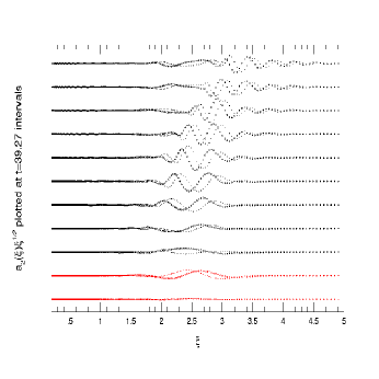
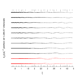
Figure 4: (a) Response of the gas disk upon applying a transient leading spiral perturbation in the $Q_{g}=1.3$ disk. Times are given in machine units (at $\xi=1$, one full revolution requires $t=39.2$) (b) Response of the gas disk upon applying a trasient leading spiral perturbation in the $Q_{g}=2.48$ disk

The effectiveness of the radial boundary conditions and the minimization of SWING amplification is shown in Figure 4a and Figure 4b which chart the progress of a simulation in which the $Q_{g}=1.3$ and $Q_{g}=2.48$ equilibrium disks are perturbed with a transient leading spiral potential (which is shut off after time $t=t_{0}$).

$${\cal V}_{1_{\rm ext}}(\xi,\varphi,t)=v_{o}\,{\rm ln}({\xi\over{10}})e^{-(\xi-\xi_{0})^{2}/h^{2}}\sin{(\pi t/t_{0})}e^{i(a{\rm ln}\xi+\omega t-m\varphi)}\,,$$ (29)

with $v_{0}=7\times 10^{-5}$, $\xi_{0}=2.5$, $h=0.5$, $t_{0}=78.4.$, and $a=6.0$. The five panels on the left show the real and imaginary components of the $m=2$ response to the the transient perturbation (scaled by $\xi^{1/2}$). Time increases from bottom to top. The entire sequence covers $n\approx 11$ full rotations at $\xi=1$. The bottom two plots show the disturbance in the disk while the perturbation is still active. In the $Q_{g}=1.3$ disk, the leading spiral propagates radially in both directions, but is only minimally amplified relative to the initial disturbance, and is largely absorbed, as desired, at the grid edges (see S00’s study of overreflection of leading disturbances in $Q_{g}\sim 1.3$ disks, which do show significant amplification, as a comparative example). In the $Q_{g}=2.48$ disk, the initial disturbance undergoes even less amplification than in the $Q_{g}=1.3$ disk, and is largely absorbed at the edges. However, we begin to see a minimal amount of numerical noise at the inner boundary after about 9 revolutions. Note that 9 revolutions at $\xi=1.0$ corresponds to $n\approx 45$ revolutions at the inner boundary. Thus, signals at the inner boundary have been transmitted more frequently than at $\xi=1.0$. Since the numerical noise is more evident at the inner boundary than at the outer boundary, and more apparent in the $Q_{g}=2.48$ disk relative to the $Q_{g}=1.3$ disk, we hypothesize that this numerical artifact scales with the frequency of signal transmissions, which is higher both at the inner boundary and in the $Q_{g}=2.48$ disk (due to its faster signal speed). This numerical noise saturates at the levels seen in Figure 4a and 4b for the $Q_{g}=1.3$ disk and $Q_{g}=2.48$ disks, respectively. Simulations run out to $n\approx 15$ revolutions at $\xi=1.0$ show no increase in the level of noise at the inner boundary, but a continued presence of this numerical artifact, which is slightly more heightened in the $Q_{g}=2.48$ disk.

6 Results

Our results divide naturally into two categories: the short-term evolution (over several hundred Myr) of the models in Table 1, and the long-term evolution (over a few Gyr) of the models in Table 2. We will use the terms branches, spurs, and feathers to describe the substructure that forms during the simulations. Our use of these terms is primarily visually motivated, but knowing the conditions in the numerical simulations that give rise to these features allows us to give the physical interpretations for their origin mentioned in § 1. By branch formation visually, we refer to the emergence of arm-like structure that spans an azimuthal range comparable to the spiral arm itself. Branches wind in the same sense as the main arms, and appear as a bifurcation of the main spiral arms. By spur formation, we refer to the appearance of structures protruding from the arms that wind in the sense opposite to that of the main arms, i.e., spurs are leading structures. These spurs are often short and stubby in appearance, as in the short-term simulations, and generally shorter in azimuthal extent than the branches. Feathers look like branches, but are shorter in length and have density contrasts only of order unity. Figures 5-16 display the surface density, along with azimuthal cuts, of the logarithm of the density response. The images shown are in terms of the radial coordinate $\xi$, as defined in the numerical procedure section. For both the short and long-term simulations, we applied the spiral potential steadily throughout the duration of the simulation. The spiral potential is turned on to full strength over a third of a revolution and held steady after reaching maximum strength. For the low $Q_{g}$ disk, corotation (CR) is at $\xi$=1.14, and the inner Lindblad resonance (ILR) and outer Lindblad resonance (OLR) are at $\xi$=0.33 and $\xi$=1.93 respectively; for the high-$Q_{g}$ disk, CR is at $\xi$=2.13, and the ILR and OLR are at $\xi$=0.623 and $\xi$=3.63 respectively. Both the logarithmic and SYL spiral planforms are applied between the ILR and OLR, while smoothed with a gaussian of the form $e^{{-(\xi-2})^{2}/0.5}$.

6.1 Short-Term Evolution: Formation of Substructure

The top panels in Figures 5-10 depict the density response at successive times in the x-y plane, where $x=\xi\cos(\phi)$ and $y=\xi\sin(\phi)$. The second panel shows corresponding azimuthal cuts of the fractional density response, i.e, $\Sigma_{\rm frac}=\Sigma(\xi,\phi,t)/\Sigma_{o}(\xi)$. Azimuthal cuts are shown at the 4:1 ultraharmonic resonance radius, along with cuts close to the resonance condition.

The third time snapshot of Model H1 shows clear branch formation. The branch appears as a bifurcation of the main spiral arms and has a smaller pitch angle than the main arms. The tighter winding of this emergent branch is in accord with the predicted effect of the second ultraharmonic as described in the Artymowicz & Lubow’s (1992) semi-analytical study, and with results from SPH simulations carried out by Patsis, Grosbæl, & Hiotelis (1997). The second time snapshot shows that when the secondary compression emerges, it is strongest relative to the main spiral arms at the $n=2$ resonance radius. Figure 1e shows that the amplitude of the secondary compression is nearly equal to the main spiral peak at $\xi=1.56$. The off-resonance $\xi=1.7$ cut indicates the presence of a secondary disturbance, but it is not as pronounced relative to the main spiral peaks at that radius. The final time snapshot shows that the bifurcation has become most pronounced at $\xi=1.7$, although a secondary compression continues to be seen at the 4:1 resonance radius. Possible reasons for the amplitude evolution of the secondary peaks at the resonant radius will be explored in the discussion section.

The second time snapshot of model H2 shows a secondary compression which is slightly more pronounced at the 4:1 ultraharmonic radius than at $\xi=1.7$. In the final time snapshot, H2 is deluged by the growth of substructure. Along with the pair of branches that is associated with the 4:1 resonance, we see a second bifurcation corresponding to the 6:1 ultraharmonic ($n=3$). The azimuthal cuts also hint at a pair of smaller compressions. H3, the non-self-gravitating analogue of model H2, develops a pair of clear branches at late times, but the density contrasts are smaller than H2’s by an order of magnitude. As before, when the branch forms, the azimuthal cut at the 4:1 resonance radius has a stronger secondary peak than the cut at $\xi=1.7$. Model HSYL, is stable to spur and branch formation and reaches arm-interarm contrasts of $\sim 4$ late in the simulation. After 2 pattern rotations, model H5 develops two, clear bisymmetric spurs with amplitudes $10\%$ those of the main spiral arms. At the last time snapshot, the spurs are most pronounced at $\xi=1.3$, which is slightly displaced from 4:1 resonant radius, $\xi=1.17$ (note that the high-$Q_{g}$ models have different resonant radii). H6, which is the non-self-gravitating analogue of H5, does not develop substructure.

In summary, the non-self-gravitating and self-gravitating models with low $Q_{g}$, namely models H1-H3, showed the development of branch-like secondary compressions. In contrast, model H5, with self-gravity and high $Q_{g}$, formed spur-like structures. The high-$Q_{g}$ model (H6) with no self-gravity showed no secondary structure. The high-$Q_{g}$ SYL model (HSYL) with self-gravity did not develop substructure during the extent of the short-term simulation. However, as the next section on long-term evolution shows, high-$Q_{g}$ models with self-gravity will not remain viable over many revolutions if the spiral forcing $\cal F$ is higher than 5%. While a secondary compression did result in the low $Q_{g}$, non-self- gravitating model, only the self-gravitating models displayed more than one secondary compression.

Some of the models in Table 1 reached extremely high density contrasts near the end of the 2.5 revolution simulations. For example, H2 and H5 attained $\Sigma_{1}/\Sigma_{0}>100.$, which is remarkable, given the decidedly small amplitude of the background forcing. In order for a disk to remain viable over the long term with an isothermal equation of state, lower forcing amplitudes are required. We note that our short and long term simulations can alternately be described as the strong and weak forcing simulations, respectively. The short term simulations have higher forcing amplitudes and evince the growth of substructure on shorter timescales, whereas the weak forcing simulations require several revolutions to display the growth of substructure.

6.2 Long-Term Evolution

Figures 11-16 show the time evolution of simulations run for 15 revolutions. The main arms of L1 can be seen to bifurcate at the second time snapshot; this arm splitting is more pronounced at $\xi=1.7$ than at the 4:1 ultraharmonic radius. At the last time snapshot, a secondary compression continues to be seen at the 4:1 resonant radius, and although the final structure is disorganized, L1 remained stable, with density contrasts $\Sigma_{1}/\Sigma_{0}\sim 1$. Model LSYL1 has developed a pair of branches in the second time snapshot, and has a flocculent appearance at the end of the simulation. LSYL1 maintained $\Sigma_{1}/\Sigma_{0}\sim 1$. Model L2 did not show branch formation and remained stable throughout. Model LSYL2, which differs from L2 only in the shape of the forcing spiral also remained stable. An incipient branch is seen in the last time snapshot. The growth of leading structures protruding from the main arms can be seen in the last timesnap for Model L3. These structures are more pronounced at radii slightly displaced from the 4:1 resonant radius. L3 remained stable for nearly the entire simulation, reaching $\Sigma_{1}/\Sigma_{0}=100$ after 14 revolutions. Model LSYL3 developed strong spurs. They are pronounced at $\xi=1.3$ in the second time snapshot. The last snapshot shows LSYL3 to have been inundated by the growth of substructure. By the time $\Sigma_{1}/\Sigma_{0}$ reached 100, nonlinear dredging had removed much of the gas from the resonant region.

In summary, spiral forcing amplitudes of 1.3-1.5$\%$ maintain a steady-state response in the $Q_{g}$=1.3 disks. The resulting spiral structure shows less organization than when the forcing amplitudes are high. The branches are strongest at radii slightly displaced from the 4:1 ultraharmonic radius. For the $Q_{g}$=2.48 disk, a 5$\%$ forcing admitted stability when the logarithmic spiral planform was used, whereas the gas became unstable when forced with the SYL spiral. As in the case of the short term simulations, the high-$Q_{g}$ disks display the development of leading structures, i.e., spurs, in contrast to the low-$Q_{g}$ disks which manifest the growth of branches. A 3.5$\%$ forcing for the $Q_{g}=2.48$ disk results in a smooth, steady-state response for both spiral planforms. It is apparent that the SYL spiral, in contrast to the logarithmic spiral, produces somewhat higher density contrasts and causes the growth of more substructure.

7 Discussion of Results

Subsequent to the identification of the ultraharmonic resonances by SMR, Artimowicz & Lubow 1992 (AL), studied the nature of these resonances in finer detail. AL’s insightful semi-analytical treatment of the dynamics of ultraharmonic resonances in the non-self-gravitating case showed that ultraharmonic waves of order $n$, which have $n$ times the wavenumber as the main arms, arise due to quadratic velocity stress terms and produce an angular momentum flux that is fourth-order in the perturbing potential, in contrast to the second-order flux that arises for the Lindblad resonances. These results demonstrate that the first ($n=2$) ultraharmonic resonance produces a bifurcation of the main spiral arms with a smaller pitch angle than the main arms. AL also gave a clear description of the higher order resonances. They found that the characteristic wavelength of the driving decreases as $\propto 1/n$ for the higher order resonances, and that resonances of high $n$ are weakened due to a combination of several effects, namely, the dependence of the response on a higher power of the driving force (assumed small), and the increasing importance of torque-cutoff effects. Finally, AL’s analysis revealed that the ultraharmonic wave acquires amplitude in a region that is centered about the location of the resonant radius, and not precisely at the resonant radius.

The azimuthal cuts presented in Figures 5-16 were made at the 4:1 ($n=2$) ultraharmonic radius along with a cut close to the resonant radius. By inspection, we find that the growth of branches and spurs, while initiated at the 4:1 resonant radius, acquired pronounced amplitude at radii slightly displaced from the resonance. This displacement agrees with AL’s analysis. AL’s semi-analytical analysis cannot however show the time development of the resonant response. This task is best accomplished by simulations. Toomre (1969) showed that linear spiral disturbances propagate radially at the usual group velocity of the wave. It is likely that the nonlinear analog of this radial propagation is responsible for the time variation we observe in the amplitude of the secondary compressions near the resonant radii. The radial spreading of the secondary compressions in model H1, for instance, between the second and last time snapshot, occurs approximately over the sound crossing time between the 4:1 ultraharmonic radius and $\xi=1.7$. Our results also differ from AL’s semi-analytic analysis by explicitly including global self-gravity. AL argued, on the basis of the conservation of angular momentum flux (e.g. Goldreich & Tremaine 1979), that ultraharmonic waves in a gas disk with only pressure will carry the same flux as in a self-gravitating disk. Our self-gravitating models, in contrast to the non-self-gravitating models, display a much greater depletion of gas in the resonant regions. Thus, we find that the angular momentum flux carried by the ultraharmonic waves is highly sensitive to the self-gravity, probably because it changes the effective amplitude of the resultant waves.

In contrast to the branches that formed for low $Q_{g}$ models, many high $Q_{g}$ models with high forcing displayed leading structures, or spurs, after several revolutions. The low $Q_{g}$ models will not remain viable for several revolutions if the forcing is comparable to that used to drive the high $Q_{g}$ disks. It is important to note that only those high $Q_{g}$ disks that were run for several dynamical times displayed spurs. For instance, HSYL is stable to spur formation at about 500 Myr. However, the long-term analogs of HSYL, like LSYL3, begin to show leading structures after about 1 Gyr. Moreover, the appearance of these structures is also highly sensitive to the level of the forcing. L2, a high $Q_{g}$ disk with a forcing of 3.5%, remains stable to spur formation. L3, also a high $Q_{g}$ disk, but with a forcing of 5%, shows clear spur formation after about 3 Gyr. In addition, the appearance of these features is also observed to depend on the type of spiral planfrom used to force the disk. LSYL2, which is analogous to L2 except that it is forced by the nonlinear SYL planform (at the same forcing amplitude as L2) displayed incipient spurs at the last timesnap while L2 remained stable througout. These observations, namely the sensitive dependence on strength of forcing, duration of simulation, and nonlinearity of planform, suggest that the traditional linear interpretation of leading features as partially reflected trailing waves off $Q$-barriers (which exist only near the corotation circle of our simulations) or by propagation through the galactic center (which is prevented by sponge boundary conditions in our simulations), may be more properly understood in some circumstances as arising from nonlinear effects.

What are some of these effects? When models are run at relatively large forcing amplitudes for many dynamical times, nonlinear dredging occurs because associated galactic shocks interior to CR produce a gradual inspiraling of the gas (Roberts & Shu 1972). The gas tends to pile up against the nearest resonance strong enough to produce such shockwaves. Such a pile-up in the local surface density then yields a barrier against the inward group motion of trailing gaseous spiral waves that are continuously being generated by the background forcing. The trailing spiral waves partially reflect from the barrier as leading spiral waves and partially transmit across it as trailing spiral waves of reduced amplitude. Gas dredging is particularly apparent in the grey scale images of H5, L3, and LSYL3. Reflection of trailing spiral waves off the sharp features just beyond the 4:1 ultraharmonic radius can then produce leading features, or spurs, while the transmitted trailing spiral waves do indeed have reduced amplitude in comparion with the incident trailing waves farther out in radius.

KO also carried out an extensive study, by performing MHD simulations, on the formation of substructure in spiral galaxies. Their analysis focused on the formation of feathers via the magneto-Jeans instability. In contrast with our simulations of low $Q_{g}$ disks, their published purely hydrodynamical models were stable to feather formation (although they clearly did simulations of unstable systems). There is no contradiction between their results and ours. KO heeded Balbus & Cowie (1985) suggestion that $Q_{\rm sp}=Q_{g}(\Sigma_{0}/\Sigma_{\rm max})^{1/2}$ is the appropriate parameter that characterizes the gaseous response to an applied perturbation. The square root appears rather than the more naive linear factor for the surface density compression behind a galactic shock because of the increase in the local postshock shear from the unperturbed state. KO first carried out 1D asymptotic calculations to construct steady spiral shock configurations that were quasi-axisymmetrically stable. In terms of the local $Q_{\rm sp}$ parameter, their 2D simulations were informed by these 1D quasi-axisymmetrically stable model to satisfy $Q_{\rm sp}>0.9$. They then found that their unmagnetized hydrodynamical models were stable to feather formation. Our 2D models are not restricted to the range $Q_{\rm sp}>0.9$, and thus could develop transient local gravitational instabilities that gave rise to feathers. KO’s magnetized models did form prominent feathers for cases where simple $Q_{\rm sp}$ considerations would have predicted stability. Evidently, magnetization destabilizes high $Q_{\rm sp}$ disks by the mechanism of shear reduction in the magneto-Jeans instability, as discussed in the linear regime by Lynden-Bell (1966), Elmegreen (1993), and Kim & Ostriker (2001). However, the MHD stability criterion is not easy to state analytically, so we will be satisfid with the loose notion that instability arises when an effective $Q_{g}$ crosses some threshold value. In any case, because the wing of feathers behind the primary shock front were all of roughly equal strength in KO’s local simulations, such feathers could not be born from ultraharmonic resonances of different forcing capability.

In a sense, therefore, our low $Q_{g}$ hydrodynamic simulations are mimicking the feathering behavior of relatively high effective $Q_{g}$ magnetohydodynamic simulations. It is important to note that the usual $Q_{g}$ does not characterize the signal speed of compressive wave propagation in the MHD context. Thus, the effective $Q_{g}$ of magnetized disks, due to the MHD modifications of the sound speed, should be considered when evaluating the response of the disk. Only high effective $Q_{g}$ disks can avoid runaway catastrophes that prevent the simulations from being carried out long enough to accumulate the ultraharmonic resonant encounters that explain branching and to develop the secular drifts that explain spur formation. Thus, we anticipate that moderately high $Q_{g}$ simulations,with the inclusion of frozen-in magnetic fields, can produce models that simultaneously exhibit branches, spurs, and feathers.

Another question that motivated this study is whether a steady ordered driving field can produce, via overlapping nonlinear effects, a disordered response in the gas. Repeated passages of gas through the spiral arms at ultraharmonic periodicities will cause secondary compressions in the form of branches and spurs that become especially pronounced for our self-gravitating models. Model H2 and LSYL3, in particular, illustrate a divergent growth of substructure that ultimately causes the systems to destabilize. We cannot, however, attribute this apparently chaotic effect to the resonance-overlap mechanism as we cannot rule out the growth of substructure via purely numerical effects in H2 and LSYL3. We have performed a high-resolution run (512x512) for H2 and find that even though it is initially convergent, the agreement with the lower-resolution run breaks down towards the end of the simulation. However, the high-resolution run that we performed for L1 maintains agreement with the lower-resolution run throughout. Thus, we can say with greater confidence that the growth of substructure in L1 is not due to numerical artifacts, whereas we cannot say this definitively for models like H2 where surface density contrasts reached $\sim 100$. The unequivocal demonstration of this phenomenon in a simulation, i.e., flocculence arising purely from overlapping nonlinear effects, will necessary require ruling out the possibility that it arose from numerical artifacts.

We have noted previously that for the same forcing amplitude, the SYL spiral planform induces the growth of more substructure than the logarithmic spiral planform. This happens despite the fact that the more open spiral winding of the SYL planform couples less naturally to the spiral response of the gas, which does not easily sustain disturbances with large radial wavelength. For instance, we note that LSYL2 shows incipient spur formation at the last timesnap, while L2 is stable to the formation of substructure. We also noted in the section on ultraharmonic resonances that the nonlinear nature of the SYL planform allows for potentially more occurrences of resonance overlap than the linear logarithmic-spiral planform. The positive correlation of a more chaotic or flocculent response for the SYL planform thus does lend credence, but not yet demonstrated assurance, to the idea that a steady, smooth driving force field can induce, over the long run, a disordered and even flocculent response in the interstellar gas clouds (and the population I stars born from them) via the mechanism of overlapping ultraharmonic resonances.

7.1 Caveats and Future Work

It is important to emphasize that since we performed whole-disk simulations with an isothermal equation of state, we can study the formation of secondary spiral structures that grow via the ultraharmonic resonances, but we cannot study the fragmentation of such structures to become self-gravitating bodies (as KO did). The reason for this is two-fold. Our global simulations do not have the dynamic range necessary to follow the development of strong feathering that lead to local fragmentation. Differential dredging could lead to similar problems locally. Moreover, global simulations admit multiple reflections off radial irregularities in the system; these can lead to accidental resonant cavities that create growing quasi-modes. In this fashion, some self-gravitating models with large spiral forcing may have developed high density contrasts in the main spiral arms that tend to destabilize the system as a whole. Model H2, for instance, illustrates the result of higher order resonances, but also reaches excessively high density contrasts.

Our simulations (and KO’s) are also limited by the isothermal equation of state. No damping mechanism other than radial drift prevents the gas from shocking repeatedly. Self-regulation from star formation and supernovae explosions may play an integral role in the realistic scenario in holding off local runaway collapse by increasing local $Q_{g}$ values. Another line of improvement in the context of purely hydrodynamical models, as suggested by KO, is a more realistic treatment of the true interstellar medium (ISM), with particular attention paid to its microscopic properties. Shu et al. (1972) made an early attempt in this direction by treating the ISM as two thermally stable phases (Field, Goldsmith, & Habing 1969) forced by an external spiral field.

The present understanding of the ISM as a highly turbulent and multiple phased medium compels a greater scrutiny and a finer treatment of the interplay among many physical effects (McKee & Ostriker 1977). In particular, the ubiquitous 3D turbulence observed in the ISM may serve to stabilize the disk even when the gas is driven by a large spiral field. Local 3D simulations developed to study magnetic and hydrodynamic self-gravitating flows indicate that some systems remain stable for conditions where a 2D treatment would have indicated instability (Kim, Ostriker, & Stone 2002)

Finally, we note that the intent of the section on long-term simulations was to consider models repesentative of long-lived spirals that have existed in relative isolation for many revolutions. We found that the repeated passage of gas through regions of ultraharmonic resonance induce in these models secondary structures akin to the branches, spurs, and feathers observed in the population I stars and gas of many external disk galaxies. The short-term simulations of high $Q_{g}$ disks at higher relative amplitudes of background spiral forcing yielded much cleaner grand-design structures in the interstellar gas. On the basis of numerical simulations by other workers starting with Toomre & Toomre (1972), a similar “cleaning up” of the otherwise messy appearance (in blue light) of normal galaxies may be accomplished by the violence of a close tidal encounter with another galaxy.

On the other hand, Block et al. (1994) point out the existence of many disk galaxies that have orderly grand-design spiral patterns when observed in the infrared, yet appear quite messy, and even flocculent, when observed in optical or blue light. They suggest that the existence of so many infrared grand-design spirals cannot be the result of occasional tidal encounters, but must almost certainly represent the quasi-stationary spiral normal-mode long postulated by C. C. Lin and collaborators to be present in the background of old disk stars (Lin & Shu 1964; Lin et al. 1969; Lin & Lau 1979; Bertin & Lin 1966). However, Block & coworkers (Block & Wainscoat 1991, Block et al 1994, 1996) also suggested that the contrasting lack of order in the population I component, and by inference, in the interstellar gas, must mean that the dynamics of the gas and old disk stars are decoupled. Our long-term simulations demonstrate that this conclusion need not follow. The gas of a disk galaxy can be driven gravitationally by an orderly spiral pattern existing in the infrared background of disk stars, and yet the nonlinear response can be disorderly and even chaotic, especially if the ordered driving lasts long enough to establish the nonlinear superposition of several overlapping ultraharmonic resonances. But better calculations are needed before we can confidently establish that truly flocculent galaxies can be constructed by the mechanisms of nonlinear dynamics alone.

8 Conclusion

Impressive displays of spiral substructure in the form of inter-arm branches, protruding spurs, and feathering between the main arms imparts a scabrous and disordered appearance to the large-scale structure of many spiral galaxies. We have performed a number of hydrodynamical simulations to study the growth of these structures in the presence of various ultraharmonic resonances. We find that self-gravity is a primary catalyst in heightening the strongest ultraharmonic, i.e., the 4:1 resonance, which produces a bifurcation of the main arms. Moreover, we see that self-gravity is crucial for the growth of substructure via the higher-order resonances. In our simulations, we strove to isolate the effects of the resonance mechanism by purposely minimizing the roles of the swing amplifier and reflection-induced feedback from inner and outer boundaries (but not ones produced by internal dredging). Our short-term simulations with large forcing amplitude generate a vigorous response in the gas, eliciting the growth of branches and feathers in the low $Q_{g}$ cases. The long-term simulations, which had lower forcing amplitudes and were run over a timescale of several Gyr, illustrated initially a smooth response in the gas that resembled the driving spiral field, but which over time, accumulated the effects of dredging and ultraharmonic resonances. Prominent leading spurs as offshoots from the secondary commpressions and dredging associated with ultraharmonic resonances are the main surprise of such long-term simulations. When combined with the speculation that high $Q_{g}$ hydromagnetic simulations mimic the feathering capability of low $Q_{g}$ hydrodynamic simulations, these results reinforce the idea that the gaseous response in disk galaxies to an ordered background spiral gravitational field becomes increasingly disordered with time, with the appearance of numerous branches, spurs, and feathers atop the main grand-design spiral arms. Background forcing planforms with a sufficiently nonlinear azimuthal dependence may even generate so many overlapping subharmonic resonances that the entire gas structure becomes chaotic and flocculent.

In the cleaner spiral galaxies, as noted in Elmegreen & Elmegreen (1990), if a number of the ultraharmonic resonances can be matched with observed features, the determination of the pattern speed of the stellar background would be on a firmer footing. However, any design study of a particular galaxy that attempts to match observed features with a given resonance must also endeavor to disentangle the effects of the two other primary mechanisms of structure formation in self-gravitating systems, namely, SWING amplification and reflection-induced feedback. As we have noted, 3D simulations that model the ISM more realistically are needed to further understand the details of the growth of substructure via resonance phenomena. Finally, the addition of a responsive stellar component would serve to demonstrate the thesis (Roberts & Shu 1972; see also AL for a related point concerning the damping associated with ultraharmonic resonances) that galactic shocks would extract energy and angular momentum from the stellar wave of a sign as perhaps to saturate its intrinsic tendency to grow as an unstable normal mode of the system. Such a program would fulfill the hope and vision embodied by the original hypothesis of quasi-stationary spiral structure proposed by Lin & Shu (1964).

We are grateful to the referee for helpful criticisms that improved the presentation of this paper. S.C. would also like to thank L. Blitz, J. Graham, W.T. Kim, M. Krumholz, C. McKee, J. Sellwood, A. Toomre, and especially C. Yuan for useful discussions and insightful criticisms. We also thank S. Dawson, C. Heiles, and E. Rosolowsky for suggestions on improving the visual presentation of the data. This research was funded in the United States by the National Science Foundation and NASA, and in Taiwan, by the National Science Council and Academia Sinica.

Figure 1: $Q$ vs $D_{\star}$ for full disk overplotted with $Q_{g}$ vs $D_{\star}$ for partial disk

Figure 2: (a)Curves of marginal stability for axisymmetric (ringlike) disturbances in partial SIDs. Heavy solid lines delineate the collapse and ring fragmentation regions for a full ($F=f=1.0$) SID. Also shown are computed curves of marginal stability for $F=f=0.9$ through $F=f=0.1$ in decrements of $F=f=0.1$. (Note that the curves showing the collapse branches for $F=f<0.7$ are outside the limits of the plot.) Our models with $Q_{g}$=2.48 and $Q_{g}$=1.3 fall in the range of oscillating disturbances. (b)Self-consistency curves for nonrotating m=2 spiral disturbances. The bottom curve is for F=f=1.0 as in S00. The upper nine curves run through F=f=0.9 to F=f=0.1

Figure 3: (a) The logarithmic spiral profile, (b) The SYL spiral profile

Figure 5: (a)-(c)Snapshot of model H1 at 95 Myr, 318 Myr, and 477 Myr, (d)-(f)Azimuthal cuts at $\xi$=1.7 and $\xi$=1.56 at times 95 Myr, 318 Myr, and 477 Myr. Solid lines denote the $\xi$=1.56 cut and the dotted lines are the $\xi$=1.7 cut. Emergent branches are marked by arrows. (a)-(c) included as jpg files. See listed website for higher resolution embedded ps figures

Figure 6: (a)-(c)Snapshot of model H2 at 95 Myr, 318 Myr, and 477 Myr, (d)-(f) Azimuthal cuts at $\xi$=1.7 and $\xi$=1.56 at 95 Myr, 318 Myr, and 477 Myr

Figure 7: (a)-(c)Snapshot of model H3 at 95 Myr, 318 Myr, and 477 Myr, (d)-(f)Azimuthal cuts at $\xi$=1.7 and $\xi$=1.56 at 95 Myr, 318 Myr, and 477 Myr

Figure 8: (a)-(c) Snapshots of model HSYL at 95 Myr, 318 Myr, and 477 Myr, (d)-(f) Azimuthal cuts at $\xi$=1.3 and $\xi$=1.17 at 95 Myr, 318 Myr, and 477 Myr

Figure 9: (a)-(c) Snapshot of model H5 at 95 Myr, 318 Myr, and 477 Myr, (d)-(f) Aziumthal cuts at $\xi$=1.3 and $\xi$=1.17 at 95 Myr, 318 Myr, and 477 Myr. Emergent spurs are marked by arrows

Figure 10: (a)-(c) Snapshot of model H6 at 95 Myr, 318 Myr, and 477 Myr, (d)-(f) Azimuthal cuts at $\xi$=1.3 and $\xi$=1.17 at 95 Myr, 318 Myr, and 477 Myr

Figure 11: (a)-(c) Snapshot of model L1 at 573 Myr, 1.91 Gyr, and 2.87 Gyr, (d)-(f) Azimuthal cuts at $\xi$=1.7 and $\xi$=1.56 at 573 Myr, 1.91 Gyr, and 2.87 Gyr

Figure 12: (a)-(c) Snapshot of model LSYL1 at 573 Myr, 1.91 Gyr, and 2.87 Gyr, (d)-(f) Azimuthal cuts at $\xi$=1.7 and $\xi$=1.56 at 573 Myr, 1.91 Gyr, and 2.87 Gyr

Figure 13: (a)-(c) Snapshot of model L2 at 573 Myr, 1.91 Gyr, and 2.87 Gyr, (d)-(f) Azimuthal cuts at $\xi$=1.3 and $\xi$=1.17 at 573 Myr, 1.91 Gyr, and 2.87 Gyr

Figure 14: (a)-(c) Snapshot of model LSYL2 at 573 Myr, 1.91 Gyr, and 2.87 Gyr, (d)-(f) Azimuthal cuts at $\xi$=1.3 and $\xi$=1.17 at 573 Myr, 1.91 Gyr, and 2.87 Gyr

Figure 15: (a)-(c) Snapshot of model L3 at 573 Myr, 1.91 Gyr, and 2.87 Gyr, (d)-(f) Azimuthal cuts at $\xi$=1.3 and $\xi$=1.17 at 573 Myr, 1.91 Gyr, and 2.87 Gyr

Figure 16: (a)-(c) Snapshot of model LSYL3 at 573 Myr, 1.91 Gyr, and 2.87 Gyr, (d)-(f) Azimuthal cuts at $\xi$=1.3 and $\xi$=1.17 at 573 Myr, 1.91 Gyr, and 2.87 Gyr

Table 1: Parameters of Short-Term Simulations

Model	$Q_{o}$	F	$\mathcal{F}$	$c_{g}/v_{rot}$
H1	1.3	0.1	2.5%	4.6%
H2	1.3	0.1	5%	4.6%
H3	$\infty$	0.1	5%	4.6%
HSYL	2.48	0.1	7%	8.8%
H5	2.48	0.1	15%	8.8%
H6	$\infty$	0.1	15%	8.8%

Table 2: Parameters of Long-Term Simulations

Model	$Q_{o}$	F	$\mathcal{F}$	$c_{g}/v_{rot}$
L1	1.3	0.1	1.3%	4.6%
LSYL1	1.3	0.1	1.5%	4.6%
L2	2.48	0.1	3.5%	8.8%
LSYL2	2.48	0.1	3.5%	8.8%
L3	2.48	0.1	5%	8.8%
LSYL3	2.48	0.1	5%	8.8%

Table 3: Resonance Parameters for low-Q models

$(\frac{m(\Omega_{p}-\Omega)}{\kappa})^{2}$	r
0.16	1.5
0.18	1.52
0.21	1.54
0.24	1.56
0.26	1.58
0.29	1.6
0.31	1.62
0.35	1.64
0.39	1.66
0.42	1.68
0.45	1.7

Table 4: Resonance Parameters for high-Q models

$(\frac{m(\Omega_{p}-\Omega)}{\kappa})^{2}$	r
0.25	1.17
0.24	1.18
0.23	1.2
0.22	1.21
0.20	1.23
0.19	1.24
0.17	1.26
0.16	1.28
0.15	1.29
0.14	1.3
0.13	1.32

References

- (1)
- (2) Artymowicz, P. & Lubow, S. 1992, ApJ, 389, 129 (AL)
- (3)
- (4) Balbus, S.A. 1988, ApJ, 324, 60
- (5)
- (6) Balbus, S.A., & Cowie, L.L. 1985, ApJ, 297, 61
- (7)
- (8) Bertin, G., & Lin, C.C 1966, Spiral Structure in Galaxies: A Density Wave Theory (Cambridge: MIT Press)
- (9)
- (10) Block, D.L., & Wainscoat, R.J., 1991, Nature, 353, 48
- (11)
- (12) Block, D.L., Bertin, G., Grosbol, P., Moorwood, A.F.M., & Peletier, R.F., 1994, A& A, 288, 365
- (13)
- (14) Block, D.L., Elmegreen, B.G. & Wainscoat, R.J., 1996, Nature, 381, 674
- (15)
- (16) Elmegreen, D.M. 1980, ApJ, 242, 528
- (17)
- (18) Elmegreen, B. G. 1993, in Protostars & Planets III, ed. E. Levy & J. Lunine (Tucson: Univ. Arizona Press), 97
- (19)
- (20) Elmegreen, B.G. & Elmegreen D.M. 1990, ApJ, 355, 52
- (21)
- (22) Evans, N. W. & Read, J. C. A. 1998, MNRAS, 300, 106
- (23)
- (24) Field, G. B., Goldsmith, D. W., & Habing, H. J. 1969, ApJ, 15, 149
- (25)
- (26) Goldreich, P., & Lynden-Bell, D. 1965, MNRAS, 130, 125
- (27)
- (28) Heiles C. 2001, in ASP Conf. Ser. 231, Tetons 4: Galactic Structure, Stars, and the Interstellar Medium, ed. C.E. Woodward, M.D. Bicay, & J.M. Shull (San Francisco:ASP), 294
- (29)
- (30) Helfer et al. 2003, ApJS, in press
- (31)
- (32) Julian, W.H., & Toomre, A.1966, ApJ, 146, 810
- (33)
- (34) Kalnajs, A.J. 1971, ApJ 166, 275
- (35)
- (36) Kim, W.T., & Ostriker, E.C. 2001, ApJ, 559, 70
- (37)
- (38) Kim, W.T., & Ostriker, E.C. 2002, ApJ, 570, 132 (KO)
- (39)
- (40) Kim, W.T., Ostriker, E.C., & Stone, J. 2002, ApJ, 581, 1080K
- (41)
- (42) Laughlin, G. 1994, unpublished PhD Thesis, U. C. Santa Cruz
- (43)
- (44) Lin, C.C., Lau, Y.Y. 1979, StAM, 60, 97L
- (45)
- (46) Lin, C. C. & Shu, F. H. 1964, ApJ, 140, 646
- (47)
- (48) Lin, C.C., Yuan, C., & Shu, F. 1969, ApJ, 155, 721L
- (49)
- (50) Lou, Y.-Q. & Shen Y. 2003, ApJ, submitted
- (51)
- (52) Lynden-Bell, D. 1966, Observatory 86, 57
- (53)
- (54) Lynden-Bell, D., & Lemos, J. P. S. 1993, astro-ph/9907093
- (55)
- (56) Mestel, L. 1963, MNRAS 126, 553
- (57)
- (58) McKee, C.F. & Ostriker, J.P. 1977, ApJ, 218, 148
- (59)
- (60) Ostriker, J. P., & Peebles, P. J. E. 1973, ApJ, 186, 467
- (61)
- (62) Patsis, P.A., Grosbol, P., & Hiotelis, N. 1997, A& A, 323, 762P
- (63)
- (64) Piddington, J.H. 1973, ApJ, 179, 755
- (65)
- (66) Roberts, W.W. 1969, ApJ, 158, 123
- (67)
- (68) Roberts, W. W. & Shu, F. H. 1972, Astrophys. Lett., 12, 49
- (69)
- (70) Shu,F., Laughlin, G., Lizano, S., & Galli, D. 2000, ApJ, 535, 190 (S00)
- (71)
- (72) Shu, F., Milione, V., &Roberts, W.W. 1973, ApJ, 183, 819
- (73)
- (74) Shu, F., Milione, V., Gebel, W., Yuan, C., Goldsmith, D.W., Roberts, W.W. 1972, ApJ, 173, 557 (SMR)
- (75)
- (76) Syer, D. & Tremaine, S. 1996, MNRAS 281, 925
- (77)
- (78) Toomre, A. 1964, ApJ 139, 1217
- (79)
- (80) Toomre, A. 1969, ApJ 158, 899
- (81)
- (82) Toomre, A. 1977, ARAA 15, 437
- (83)
- (84) Toomre, A. & Toomre, J. 1972, ApJ, 178, 623
- (85)
- (86) Toomre, A. 1981, in Structure and Evolution of Normal Galaxies, ed. S.M. Fall & D. Lynden-Bell (Cambridge: Cambridge Univ. Press), 111
- (87)
- (88) Toomre, A. 1990, in Dynamics and Interactions of Galaxies, ed. Wielen, R. (Heidelberg: Springer Verlag), 292
- (89)
- (90) Toomre, A. & Kalnajs, A.J. 1991, in Dynamics of Disk Galaxies, ed. Sundelius, B. (Goteberg, Sweden), 195
- (91)
- (92) Visser, H. 1980, A& A, 88, 149
- (93)
- (94) Woodward, P. 1975, ApJ, 195, 61
- (95)
- (96) Wong, T. & Blitz, L. 2002, ApJ 569, 157
- (97)
- (98) Zang, T. 1976, unpublished PhD thesis, MIT
- (99)