The Evolution of Protoplanetary Disk Edges

Abstract

We investigate gap formation in gaseous protostellar disks by a planet in a circular orbit in the limit of low disk viscosity. This regime may be appropriate to an aging disk after the epoch of planet formation. We find that the distance of planet to the gap outer boundary can be between the location of the $m=2$ and $m=1$ outer Lindblad resonances. This distance is weakly dependent upon both the planet’s mass and disk viscosity. We find that the evolution of the disk edge takes place on two timescales. The first timescale is set by the spiral density waves driven by the planet. The second timescale depends on the viscosity of the disk. The disk approaches a state where the outward angular momentum flux caused by the disk viscosity is balanced by the dissipation of spiral density waves which are driven at the Lindblad resonances. This occurs inefficiently however because of the extremely low gas density near the planet. We find that the distance between the planet and the peak density at the disk outer edge is only weakly dependent on the viscosity and planet mass, however the ratio of the gas density near the planet to that in the disk (or the slope of density along the disk edge) is strongly dependent upon both quantities. We find that the disk density profile along the edge scales approximately with disk viscosity divided by the square of the planet mass. We account for this behavior with a simple scenario in which the dissipation of angular momentum from the spiral density waves is balanced against diffusion in the steep edge of the disk.

1 Introduction

The discovery of extra-solar planetary systems (Mayor & Queloz, 1995) has driven a flood of renewed interest in planetary formation and disk evolution models. The focus of many models has been on mechanisms that couple the planets to the evolution of protostellar disks, the tidal interactions between a planet and a protoplanetary disk (Artymowicz & Lubow, 1994; Ogilvie & Lubow, 2002) and resulting planetary migration (Lin & Papaloizou, 1986; Trilling et al., 1998; Nelson et al., 2000; Murray et al., 1998). Gaps and holes in protostellar disks in some cases have been detected through the study of spectral energy distributions (Rice et al., 2003; Calvet, 2002; Koerner, Sargent & Beckwith, 1993) and direct imaging (Jayawardhana et al., 1998; Augereau et al., 1999; Weinberger et al., 1999; Grady et al., 2001). Since structure in protostellar disks can arise through the gravitational interaction between the disk and planets, detailed studies of these disks may allow us to place constraints on the properties of the planets in them and on the evolution of these systems.

The formation of gaps in gaseous or planetesimal disks has a long history of theoretical study. It has long been postulated that an external time dependent gravitational potential, such as from a satellite or planet, could resonantly drive waves at Lindblad resonances (LRs) in a gaseous or planetesimal disk (Goldreich & Tremaine, 1978, 1979; Lin & Papaloizou, 1979, 1993; Ward, 1997). Because these waves carry angular momentum, they govern the way that planets open gaps in disks (e.g., Bryden et al. 1999; Artymowicz & Lubow 1994) and can result in the orbital migration of planets (e.g., Nelson et al. 2000). Previous works have derived and numerically verified conditions for a planet to open a gap in a gas disk (e.g., Bryden et al. 1999). These studies focused on when gaps occur and explored the accretion rate through the gap as material was cleared to either side. Emphasis was also placed on the relationship between gap properties, accretion and orbital migration rates (e.g., Kley 1999; Nelson et al. 2000).

However, little numerical work has focused on the expected sizes and depths of the gaps in different physical regimes. Such studies are warranted because, as discussed above, gaps and holes in protoplanetary disks are detectable and so will in principle allow us to place constraints on the properties of the planets that are responsible for maintaining them.

The physical properties of protoplanetary disks should vary as the disk ages. We parametrize the disk viscosity, $\nu$, with a Reynolds number, ${\cal R}\equiv r^{2}\Omega/\nu$ where $\Omega$ is the angular rotation rate of a particle in a circular orbit around the star and $r$ is the radius. Using an $\alpha$ form for the viscosity,

$${\cal R}=\alpha^{-1}\left({v_{c}\over c_{s}}\right)^{2}=\alpha^{-1}\left({r\over H}\right)^{2}$$ (1)

where $c_{s}$ is the sound speed, $H$ is the vertical scale height of the disk and $v_{c}=r\Omega$ is the velocity of a particle in a circular orbit. We expect that the sound speed and vertical scale height of a cooling gaseous disk will drop with time, increasing the Reynolds number. For a planetesimal disk, the effective viscosity depends upon the opacity, $\tau$, (or area filling factor) of the disk with $\alpha\sim{\tau\over 2}$ in the limit of low $\tau$ (e.g., Murray & Dermott 1999 and citations within). As planetesimals coagulate or are scattered out of the disk, we expect a decrease in the viscosity and so an increase in the Reynolds number.

When viscous forces are overcome by the angular momentum flux driven by density waves, a gap in the disk near the planet opens. So as protoplanetary disks age (and their viscosity drops) we expect that gaps caused by planets will widen and accretion onto these planets will cease (Bryden et al., 1999; Kley, 1999). Because of the longer timescale associated with the end of accretion, it may be that forthcoming surveys will be dominated by partially cleared disks. The advent of new instruments such as SIRTF, ALMA, SMA and VLTI make a study of this limit particularly interesting and relevant (e.g., Wolf et al. 2002).

In this paper we numerically investigate the properties of gaps, exploring a larger range of parameter space than have previous studies. In particular we extend our simulations toward the low viscosity limit, which may govern a longer timescale in the evolution of protoplanetary disks. We critically review our results in the context of previous theories of gap formation and attempt to extend these models to embrace our new results. In a follow up paper we will explore the observational properties of our simulated disks (Varnière et al., 2004).

The structure of our paper is as follows. In section 2 we review the theory of gap formation. In section 3 we present our numerical methods and the input conditions for our models. In section 4 we present our results and in section 5 we present a critical discussion of the results along with attempts to extent previous gap formation models. A discussion and conclusion follows in section 6.

2 Previous Theory

Linear theory has been developed to predict the angular momentum flux driven by spiral densities waves exited by a planet, (Goldreich & Tremaine, 1978; Donner, 1979; Lin & Papaloizou, 1979; Artymowicz, 1993). This theory has successfully been used to predict the formation of gaps seen in numerical simulations (Lin & Papaloizou, 1993; Bryden et al., 1999). If a gap is opened then the angular momentum flux resulting from spiral density waves can be balanced by the angular momentum flux caused by the viscosity of the disk. To theoretically account for these phenomena, we require expressions for the angular momentum flux due to both processes.

As have previous works, we assume that the perturbing gravitational potential from the planet can be expanded in Fourier components

$$\Phi(r,\theta,t)=\sum_{m}W_{m}(r)\exp\left(im(\theta-\Omega_{p}t)\right)$$ (2)

where $\Omega_{p}$ is the angular rotation rate of the pattern, and $r,\theta$ are polar coordinates in the plane containing the planet. Here $\Omega_{p}$ is the angular rotation rate of a planet which we assume is in a circular orbit. The torque $T_{m}$ exerted at the $m$-th Lindblad resonance into a disk of surface density $\Sigma$ was found to depend solely on the radial profile of the perturbing potential and be independent of the process of dissipation providing that the waves are completely dissipated (Goldreich & Tremaine, 1978; Donner, 1979; Lin & Papaloizou, 1979; Artymowicz, 1993),

$$T_{m}=-m\pi^{2}\Sigma{|\Psi_{GT}|^{2}\over rdD_{m}/dr}$$ (3)

where

$$\Psi_{GT}=r{dW_{m}\over dr}+{2m\Omega\over m(\Omega-\Omega_{p})}W_{m}$$ (4)

and

$$D_{m}=\kappa^{2}-m^{2}(\Omega-\Omega_{p})^{2}.$$ (5)

Here $\Omega$ and $\kappa$ are the angular rotation rate and epicyclic frequency of an unperturbed particle in a circular orbit and are functions of radius. The above torque results from $m$-armed waves driven at the $m$th Lindblad resonance which is located at a radius determined by $D_{m}(r_{LR})=0$. Equation(3) is evaluated at this radius.

For a planet in a circular orbit, the Fourier components of the potential exterior to the planet are

$$W_{m}=-{GM_{p}\over r}b^{m}_{1/2}(r_{p}/r)$$ (6)

where $b^{m}_{1/2}$ is the Laplace coefficient (e.g., see Murray & Dermott 1999) and $r_{p}$ is the radius of the planet from the central star. We write equation (3) in the form

$$T_{m}=-f_{m}\Sigma r_{p}^{4}\Omega_{p}^{2}\left({q\over 10^{-3}}\right)^{2}$$ (7)

where $f_{m}$ are unitless constants, $q\equiv M_{p}/M_{*}$ is the mass ratio of the planet to the central star, and $\Sigma$ is evaluated at the Lindblad resonance. Evaluating equation(3) using summations for the Laplace coefficients (e.g., Murray & Dermott 1999) we find that $f_{1}=10^{-5.1}$, $f_{2}=10^{-4.3}$, $f_{3}=10^{-3.7}$ and $f_{4}=10^{-3.4}$. These values will be used in section 4 in our discussion on clearing timescales and in section 5 in our discussion on the edge profile.

If the planet is sufficiently massive and the disk viscosity sufficiently low, the torque caused by the excitation of spiral density waves will overcome the inflow due to viscous accretion in the disk and a gap will open. The angular momentum flux or torque transferred through a radius $r$ in a Keplerian viscous disk with constant viscosity and density is given by

$$T_{\nu}=3\pi\Sigma\nu r^{2}\Omega.$$ (8)

Previous estimates of gap opening criteria have applied equation(3) in the limit for large $m$ so that the resonances closest to the planet are taken into account (Lin & Papaloizou, 1979; Bryden et al., 1999). In these cases the total torque resulting from summing the resonant terms from each outer Lindblad resonance (OLR) within a distance $\Delta$ from the planet yields

$$T\approx 0.23q^{2}\Sigma r_{p}^{2}\Omega^{2}\left(\frac{r_{p}}{\Delta}\right)^{3}$$ (9)

where $r_{p}$ is the radius of the planet (Lin & Papaloizou, 1993). In what follows we take $\Delta$ to be the distance from the planet to the gap outer boundary. The expression above is valid when the gap is larger than the maximum value of the disk scale height ($\Delta>H$). When the torque from the dissipation of the outward going density waves is balanced by the torque from viscous accretion (equation 8) one can derive a criterion for gap formation, i.e. $q>40/{\cal R}$ (Bryden et al., 1999).

Once a gap is opened, the torque from viscous accretion must be balanced by the total torque from the spiral density waves driven at Lindblad Resonances exterior to the gap. As the mass of the planet increases and the viscosity decreases, the gap edges moves away from the planet so that the total torque contains fewer resonant terms. Past the $m=2$ OLR at $r\sim 1.3r_{p}$ only the weaker $m=1$ OLR at $r\sim 1.6r_{p}$ can drive spiral density waves. Previous works have suggested that the location of the $m=2$ OLR resonance would set the radius of disk edges in low viscosity disks harboring large mass planets (Lin & Papaloizou, 1993). It is possible that as the gap is cleared, gas could accumulate near this resonance (Lin & Papaloizou, 1993). Alternatively, spiral density waves could be driven at a LR via a ‘virtual effect’ as long as the resonance was within a particular distance of the disk edge. This argument has been used to provide a possible explanation for $m=2$ structure seen in simulations of binaries (e.g., Lin & Papaloizou 1993, 1979; Savonije et al. 1994). A large mass ratio, such as would be found in a stellar binary system, or extremely small disk viscosity, is required to open a gap out to the $m=1$ OLR in a circumbinary disk (Artymowicz & Lubow, 1994).

The balance between torque from spiral density waves and $T_{\nu}$ should allow one to derive a scaling relation for the gap width. If we naively use equation (9) and assume a Keplerian rotation profile, we find

$$\Delta=0.29q^{2/3}{\cal R}^{1/3}r_{p}.$$ (10)

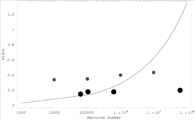
Figure 1: Disk width vs Reynolds number. The $y$-axis shows the distance from the planet to the outer disk edge. The $x$-axis shows the Reynolds number. The solid line shows the prediction based on equation 10. Large points are measured from simulations displayed by Bryden et al. (1999). Small points are taken from simulations shown in this paper with planet mass ratio $q=10^{-3}$. Note that the definition of the gap width differs slightly for the two points (see section 4.1). This plot demonstrates that simple models (such as based on equation 10) fail to predict the dependence of gap width on viscosity.

While previous numerical studies have confirmed the condition for opening a gap, a general scaling relation to predict the gap width has not yet been developed. However, it is possible to extract some information from published data in order to probe the scaling of gap width with planet mass and disk viscosity. In Figure 1 we present a plot of equation(10) along with data from Bryden et al. (1999) as well as data from our own simulations. The points by Bryden et al. (1999) were taken for their $q=10^{-3}$ simulations and the gap widths were measured from their density profile plots. The gap width was taken to be the distance from the planets orbital radius to the location along the outer gap wall where the density is half of that outside the gap. Reynolds numbers were computed using their quoted values of the viscosity parameter $\alpha_{ss}$ and

$$\nu=\alpha_{ss}(H/r)^{2}r^{2}\Omega.$$ (11)

For the zero viscosity case of Bryden et al. (1999), we use their quoted value of the numerical viscosity yielding $\alpha_{ss}=10^{-5}$.

Inspection of Figure 1 shows that the scaling relation given in equation (10) produces the correct order of magnitude gap width. Equation(10), since it is based upon a high $m$ integration, is correct for lower planet masses and higher disk viscosities, providing an explanation for the correct positions of the points in Figure 1 on the high viscosity end. Given that the gap edge is not sharp, there is some ambiguity in the definition of $\Delta$ and hence in the exact comparison between equation(10) and the simulations. We take up this point again in section 4. In spite of this uncertainty, the failure of the scaling relation to predict the gap width across a wide range of Reynolds numbers is clearly seen in the trend shown by the simulations of Bryden et al. (1999). The gap width increases more slowly than predicted by equation(10) and is off by a factor of $2$ or more at low viscosity. Again this is consistent with the fact that equation(10) does not appropriately estimate gap widths when the edge of the disk is near the lower order Lindblad resonances. It is difficult to draw firm conclusions from this data since Bryden et al. (1999) do not explore the relation across a uniform (in log) sampling of viscosities. Figure 1 also shows data from our simulations with a more complete sampling of viscosity and these confirm the weak dependence of gap width on Reynolds number.

Thus it appears that while previous approaches can predict when a gap forms they do not capture the full physics of the gaps. In particular some aspect of the scenario in which the torque from waves driven at the OLR is balanced by viscous accretion (as discussed by Bryden et al. 1999) must be incomplete. This is not a trivial point as observational diagnostics from platforms such as SIRTF and ALMA may determine gap widths to less than 10% (Wolf et al., 2002). Since many of the observable systems may be appropriate for the low viscosity limit, understanding the proper scaling there will be critical to using observations of gap widths and disk edges to infer protoplanet properties.

3 Numerical Code Description

To investigate the evolution of gaps opened by a protoplanet, we ran a set of $2$D hydrodynamical simulations using the code developed by Masset (2002); Masset & Papaloizou (2003). This code is an Eulerian polar grid code with a staggered mesh and an artificial second order viscous pressure to stabilize the shocks (see also Stone & Norman 1992). The hydrocode allows tidal interaction between one or more planets and a 2D non-self-gravitating gaseous disk, and is endowed with a fast advection algorithm that removes the average azimuthal velocity for the Courant timestep limit (Masset, 2000). The simulations are performed in the non-inertial non-rotating frame centered on the primary star (similar to a heliocentric frame). The outer boundary does not allow either inflow or outflow, so it must be located sufficiently far from the planet to ensure that spiral density waves are damped before they reach it. This is facilitated by adopting a logarithmic grid in radius. The grid inner boundary only allows material to escape so that the disk material may be accreted on to the primary star.

The code is scaled so that the unit length is $1$ AU which is the initial position of the protoplanet, the unit mass is $1\ M_{\odot}$, which is the mass of the central star, and time is given in units of one orbital period (one year) for an object in a circular orbit at the initial location of the planet.

The runs we are presenting here are made with a resolution of $N_{r}=150$ and $N_{\theta}=450$. The grid physical size spans radii between $0.25$ AU and $6.0$AU. The viscosity is parametrized with the Reynolds number ${\cal R}\equiv r^{2}\Omega/\nu$, where $\cal R$ is assumed to be constant with radius. The disk aspect ratio $H/r=0.04$ is uniform and constant where $H$ is the vertical scale height of the disk. The sound speed of the gas is set from the disk aspect ratio. The planet was initially embedded in a disk with density profile $\Sigma(r)=10^{-5}\left({r\over R_{min}}\right)^{-1.5}$ where $R_{min}$ is the radius of the inner edge of the grid. Table 1 shows the characteristics of each run we will discuss here.

4 Results

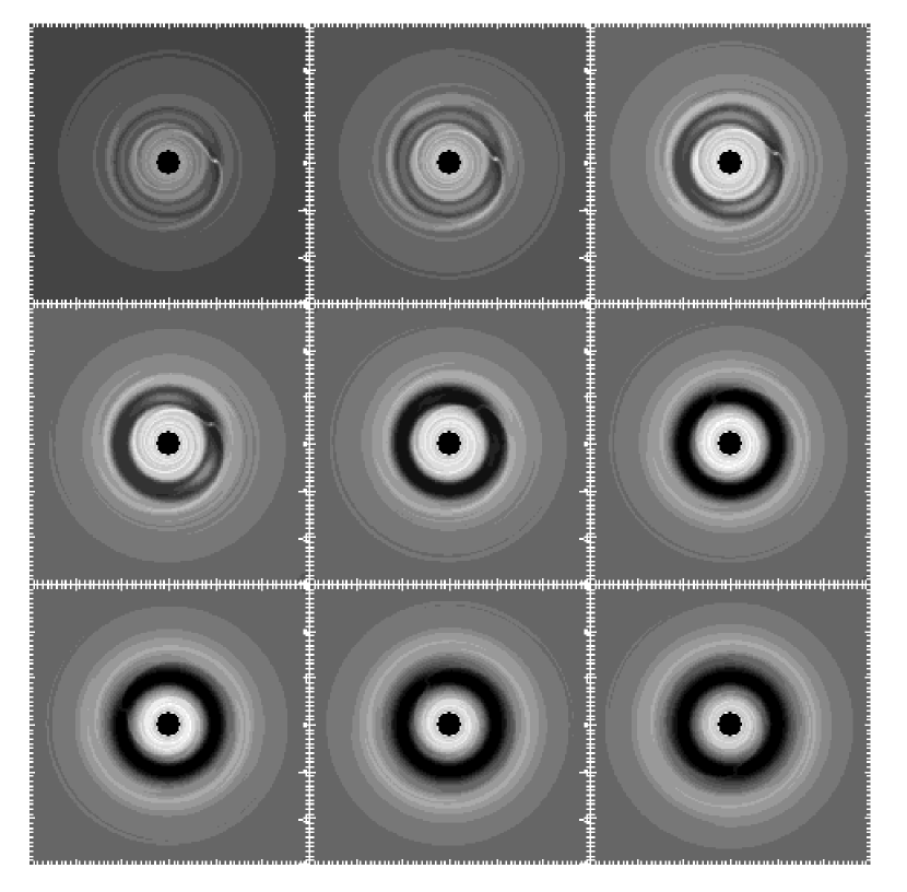
Figure 2: 2-D simulation of a $q=10^{-3}$ (approximately Jupiter mass) planet opening a gap in a gas disk with Reynolds number ${\cal R}=2\times 10^{6}$. The gas density is shown at times 10, 20, 50, 100, 200, 500, 1000, 2000, and 3000 after the beginning of the simulation. Times are given in units of rotational period of the planet around the star. The top three panels show the initial clearing of the gap on a fairly short timescale. The bottom three panels show the longer timescale behavior. On long timescales the gap opened by the planet is between the $m=2$ and $m=1$ OLR.

Figure 2 show snapshots of the density for a typical simulation, namely $q=10^{-3}$ (corresponding to a Jupiter mass planet) and a Reynolds number ${\cal R}=2\times 10^{6}$. From top to bottom and left to right we show the density distribution at times $t=20,50,100,200,500,1000,2000$ and 3000 (in units of the planet’s orbital period). We see that a gap is cleared relatively quickly during the first hundred rotation periods. During this time period a prominent 2-armed structure is seen in the density distribution. At later times, the density near the planet drops and the amplitude of the spiral density waves decreases. An asymptotic state is approached on longer timescales when the edge of the disk is between the $m=2$ and $m=1$ OLRs. We see that the gas interior to the planet slowly accretes onto the star while that exterior to the planet slowly accretes inward piling up near the edge of the disk, outside the planet.

The shape of the disk edge at latter times is better seen on Figure 3a which shows the density profile of the inner region of the disk for the same sampled times. Figure 3a also shows 3 radial functions that can be used as metrics to measure $\Delta$, the “outer” width of the gap or the distance between the planet and the gap outer edge.

4.1 Measuring the distance between the planet and the edge of the disk

To measure the distance between the planet and the edge of the disk from a numerical simulation we must first consider procedures for defining a point of measurement for the disk edge. As seen in Figure 3a, the gaps are not well approximated by a square well. Figure 3a illustrates three procedures for defining a location to measure the disk edge from a radial density profile. In each case we choose a stationary radial function and define $\Delta$ based on the location where the radial density profile crosses this function. Our first case, defined by the upper line in Figure 3, is the initial unperturbed density profile. For the second case we use one half of the initial density profile to define our points of measurement. Our third case (represented by the horizontal line in Figure 3) is defined with an absolute density of $\Sigma=10^{-6}$ (independent of radius) which is approximately an order of magnitude below the initial disk density at $r=r_{p}$.

We now compare the evolution of $\Delta$ based on these measurements. From Figure 3b we see that the second and third definitions evolve similarly, but the first one, which refers to the initial density profile, continues to increases on long timescales to a greater extent than the other measurements. Because accretion continues from the outer parts of the disk, the gas density at the outer boundary of the gap continues to increase on long timescales. It is likely that this slow accretion governs the longterm behavior at the “top” of the density profile. To minimize the sensitivity to the exact shape of the edge profile we subsequently choose to measure the distance between the planet and the edge of the disk using our third measurement case (referring to an absolute density of $\Sigma=10^{-6}$). Because there are no significant differences between the second and third measurements, we have chosen to subsequently measure the simpler of the two.

4.2 Evolution of the disk edge

Figure 4 shows the evolution of $\Delta$, the distance between the planet and the disk edge, and the density at the location of the planet for three simulations (runs #6, #8 and #11 listed Table 1) which share either the same planet mass ratio or viscosity. The starred points show the depth and width for a planet mass ratio of $q=2\times 10^{-3}$ in a disk with ${\cal R}=2\times 10^{6}$. We refer to this run as the “reference run”. The crosses show a run that has the same Reynolds number but a planet mass ratio $q=10^{-3}$, half that of the reference run. The last simulation (shown with diamond points) has the same planet mass ratio as the the reference run but a higher disk viscosity (${\cal R}=2\times 10^{5}$).

Our initial density distribution, that of a smooth power law, is not an equilibrium state in the presence of a planet. As previous numerical studies have illustrated, the planet accretes gas and tidally induces spiral density waves that repel the gas from the planet. Figure 4 shows that two regimes govern the evolution of the depth and width of the gap. On short timescales ($t<200$ orbital periods) the clearing of gas near the planet is rapid. The depth of the gap is almost independent of the planet mass and viscosity, however the distance between the planet and the gap outer boundary of the disk is dependent upon both. After $t\sim 200$ orbital periods, both the density and gap width evolve much more slowly, as if approaching a steady state.

A careful inspection of Figure 4 shows that the initial evolution of the simulations are very similar, and nearly independent of the disk viscosity. This suggests that at early times the angular momentum flux is dominated by spiral density waves driven by the planet, and that the viscous inflow rate is relatively minor. The clearing of the initial gap should take place on a timescale that is set by how fast the spiral density waves can push mass away from the planet. The torque on the disk can be estimated from the sum over each resonance outside the edge of the disk. If the density drops near the planet, then the Lindblad resonances nearest the planet will not significantly contribute to the torque on the disk. In other words, because equation (3) depends on the density at the resonance, only resonances outside the gap in the disk will exert a significant torque on the disk.

At the beginning of the simulation the gas disk extends all the way to the Roche lobe of the planet and the clearing timescale is set by a summation over high order (large $m$) Lindblad resonances. However as gas is cleared away from the planet, the density drops at the highest order resonances and the lower order Lindblad resonances take over. Since these aren’t as strong, this clearing should go at a slower rate. So we expect that much of the clearing takes place under the influence of only the last few resonances. From equation(7) we expect evolution on a timescale in planetary rotation periods

$$t_{clear}\sim{r_{p}^{4}\Omega_{p}^{2}\Sigma\over 2\pi\sum_{m}T_{m}}\sim 250\left({q\over 10^{-3}}\right)^{-2}$$ (12)

where we have added the contributions from the $m=$2,3 and 4 Lindblad resonances.

When the gap opens sufficiently that the higher order resonances are evacuated and the $m=2$ OLR resonance dominates, the timescale could be an order of magnitude longer. Nevertheless, the above timescale is approximately what we see for the first phase of evolution from the simulations presented in Figure 4, and is consistent with this first phase of evolution being independent of the disk viscosity. Since the timescale for clearing the gas away from the planet depends primarily on the planet mass, we expect that the simulations with massive planets will initially clear material faster than those with lower mass planets. This is primarily seen in the evolution of the disk edge (Figure 4b) and not in the depth of the gap (Figure 4a), though the depth of the gap in the lower planet mass simulation (crosses) is higher than that of the higher planet mass simulation at the same viscosity (stars).

On longer timescales viscous behavior becomes important. For the higher viscosity simulations we expect the viscosity becomes important earlier on, consistent with the quicker transition toward the regime of slower evolution seen in the higher viscosity simulation (diamonds) in both density and width plots of Figure 4. Except for the lowest viscosity simulations considered in this paper, the transition to the longer slower evolution takes place near $t=200$ orbital periods. So measurements taken after this time can be considered to represent quantities measured when the disk is slowly evolving. Because accretion continues from the outer disk, gas continues to pile up at the edge of the disk. Consequently these simulations never reach a steady state, but on long timescales slowly evolve on the viscous timescale of the outer disk.

The long term accretion complicates the development of an understanding of the scaling behavior of the edge profile on planet mass and disk viscosity. To enable us to explicate the dependence of the disk edge profile on planet mass and disk viscosity we will subsequently compare gap properties measured at different times and discuss the scaling of the properties of disk edges keeping in mind that our simulations show evolution on two timescales.

4.3 Influence of the disk’s viscosity

Figure 5 shows the depth and distance to the edge of the disk for a simulation with planet mass ratio $q=2\times 10^{-3}$ as function of the Reynolds number. The upper curve (diamond points) is at $t=200$, i.e. in the first phase of evolution. The lower curve (starred points) is at $t=1000$, and shows the second phase of evolution. At latter times when the viscous timescale becomes important, we see that the depth is more strongly influenced by the disk viscosity than during the first phase. The depth at $t=200$ is independent of viscosity for ${\cal R}\gtrsim 10^{6}$ because the secondary timescale evolution has not yet completely taken over (see Figure 4).

Although the gas density near the planet is strongly dependent on the viscosity at later times, the distance between the planet and the edge of the disk is only weakly dependent upon the disk viscosity (see Figure 5b). A variation of 2 orders of magnitude in the disk viscosity causes only a 30% change in the distance between the planet and disk edge, but a similar scale (2 orders of magnitude) variation in the gas density. The strong dependence of the gas density near the planet on viscosity, and weak dependence of the actual location of the disk edge on the disk viscosity will be discussed in section 6 when we consider modifications to the previous theory.

4.4 Influence of the protoplanet’s mass

Figure 6 shows the behavior of the gap and disk edge created in a disk of viscosity corresponding to ${\cal R}=2\times 10^{6}$ as function of the planet mass ratio. We plot results for simulations carried out with planet mass ratios between $q=10^{-4}$ and $2\times 10^{-3}$. The two lines shown in both figure panels are similar so we can study the dependence of the gap density and width on the planet mass ratio without being sensitive to the time at which the measurements were taken.

We see from Figure 6 that both the depth and the distance between the planet and disk edge vary significantly as function of the planet mass even though we have only run simulations over a relatively small range in planet mass ratio (particularly when we compare to the larger range of Reynolds numbers that we explored). Since a gap will not open at the lowest planet masses and higher ones exceed the masses of most known extrasolar planets, we cannot significantly extend the range of planet masses considered. In the regime plotted in Figure 6 we see that a variation in the planet mass ratio of a factor of 4 causes approximately an order of magnitude a change in the gas density near the planet, and a 40-50% change in the distance between the planet and the disk edge. As we previously found for the dependence on disk viscosity, the distance between the planet and the disk edge is less strongly dependent upon the planet mass ratio than is the gas density near the planet. Both the depth and distance between the planet and disk edge are more strongly dependent upon the planet mass ratio than on the disk Reynolds number. In the following section we will attempt to account for the trends we observe in the long timescale evolution of these simulations.

5 Comparisons to Theory

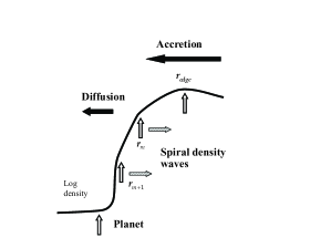
Figure 7: We expect that diffusion or viscous spreading is important in the steep edge of the disk. Arrows represent the direction of the mass flux. The torque from dissipated spiral density waves is balanced by by diffusion in the steep edge of the disk. To maintain a balance, the density at the resonance can be very low. In the regime where the distances between the resonances is smaller than the dissipation scale length, each resonance cases a change in the slope of the density profile.

As suggested by Bryden et al. (1999), when mass has been removed from the region nearest the planet and a steep density gradient is present, diffusion or viscous spreading may become important and determine the shape of the edge of the disk (see Figure 7). The basic equation that describes the evolution of a Keplerian disk due to viscous processes is

$${\partial\Sigma\over\partial t}={3\over r}{\partial\over\partial r}\left[r^{1/2}{\partial\over\partial r}\left(\nu\Sigma r^{1/2}\right)\right]$$ (13)

(Pringle, 1981). This equation arises by considering the Navier-Stokes equation and conservation of mass. The azimuthal component of the Navier-Stokes equation, which addresses angular momentum transport, is used to estimate the radial velocity component. This, when inserted into the equation for conservation of mass, yields the above equation. When the density $\Sigma$ is nearly flat, the angular momentum flux or torque through a radius $r$ is given by equation(8). This is what is usually meant by “accretion,” as we shall see. When the radial gradient of $\Sigma$ is very large however, there is an additional diffusive term that drives mass flow.

The previous equation can be modified to include mass and angular momentum flow due to dissipation of spiral density waves driven by the planet by adding a term,

$${\partial\Sigma\over\partial t}={3\over r}{\partial\over\partial r}\left[r^{1/2}{\partial\over\partial r}\left(\nu\Sigma r^{1/2}\right)+{1\over 3\pi r\Omega}\sum_{m}{\partial F_{m}\over\partial r}\right]$$ (14)

where ${\partial F_{m}\over\partial r}$ corresponds to the torque density exerted in the disk due to dissipation of spiral density waves driven by the planet at the $m$th Lindblad resonance, and there is a sum of terms due to the contributing resonances. Here we have followed the derivation by Takeuchi et al. (1996).

Once a prominent gap is opened we must distinguish between the physics occurring within the gap, (particularly along its steep outer edge), and that occurring outside the gap edge at larger radii. Outside of the gap the density gradient is shallow, the diffusion rate will be small and we expect that the mass inflow due to accretion will dominate and will be balanced by mass outflow resulting from the spiral density waves. However, in the steep edge itself, diffusion should be important. In this region it is mass inflow due to diffusion that should be balanced by the mass outflow caused by dissipation of the spiral density waves. Thus we can divide the problem into two regimes: accretion dominated and diffusion dominated (see Figure 7). This division can be directly seen in Figure 3a showing the density profile of a single simulation. Past the edge of the disk ($r\sim 1.3$) the density gradient is small, but inside this radius, the density drops by orders of magnitude and the density gradient is large.

Unless the planet mass is sufficiently low and viscosity sufficiently high that a gap is only barely opened, we expect that edge of the disk will be steep. The resonance most distant from the planet at highest density $\Sigma$ should dominate the shape of the outer part of the edge because it will be most effective at driving spiral density waves. We refer to quantities such as radius and density past the edge of the disk as $r_{e}$ and $\Sigma_{e}$ and those at the $m$-th OLR resonance as $r_{m}$ and $\Sigma_{m}$ (see Figure 7).

In the limit that the density is not varying quickly with time, (${\partial\Sigma\over\partial t}\approx 0$), the previous equation can be written

$${3\nu}\Sigma+3\nu r{\partial\Sigma\over\partial r}\sim-{1\over 3\pi r\Omega}\sum_{m}{\partial F_{m}\over\partial r}+{\rm constant}$$ (15)

where the first term on the left is what is typically known as accretion and the second can be described as diffusion. Here $F_{m}$ is the angular momentum flux transfered by the waves and $-{\partial F_{m}\over\partial r}$ is the torque density exerted on the disk due to the dissipation of the waves in the disk (Takeuchi et al., 1996). Using the definition for the Reynolds number, we can rewrite the previous equation as

$${\partial(r\Sigma)\over\partial r}\sim-{{\cal R}\over 3\pi GM_{*}}\sum_{m}{\partial F_{m}\over\partial R}.$$ (16)

Integrating the previous equation we find

$$r\Sigma\sim-\sum_{m}{{\cal R}F_{m}\over 3\pi GM_{*}}+{\rm constant}$$ (17)

which implies that the shape of the disk edge is entirely determined by the way that the waves are dissipated. The steep edges we see in the simulations imply that the dissipation occurs very rapidly, as previously pointed out by Takeuchi et al. (1996).

The angular momentum flux transferred by the spiral density waves $F_{m}$ is equal to that given by equation (3) at the location of the resonance $r_{m}$ and then decays because of dissipation. We assume that the spiral density waves are dissipated over a length scale $r_{d}$ (referred to as a damping length by Takeuchi et al. 1996), so $F_{m}\sim T_{m}(1-e^{-(r-r_{m})/r_{d}})$ for $r>r_{m}$ and $T_{m}$ is given by equation (7) with quantities defined at the resonance. We associate the edge of the disk as that point where the dissipation of the density waves ceases to be important; $r_{e}\sim r_{m}+r_{d}$ where $r_{m}$, in this case, is the outermost resonance that still lies within the disk edge.

Considering only one resonance we can rewrite the previous equation as

$$r\Sigma\sim r_{m}\Sigma_{m}+{{\cal R}\Sigma_{m}f_{m}r_{p}\over 3\pi}\left({q\over 10^{-3}}\right)^{2}\left(1-e^{-(r-r_{m})/r_{d}}\right)$$ (18)

for $r>r_{m}$. We expand this to include all resonances.

$$r\Sigma\sim r_{p}\Sigma_{p}+\sum_{m}{{\cal R}\Sigma_{m}f_{m}r_{p}\over 3\pi}\left({q\over 10^{-3}}\right)^{2}a_{m}(r)$$ (19)

where

$$a_{m}(r)= 0 {\rm for}~{}~{}~{}r<r_{m}$$ (20)

$$1-e^{-(r-r_{m})/r_{d}} {\rm for}~{}~{}~{}r>r_{m}.$$

First let us consider the outermost resonance that still lies within the edge of the disk. Since the rightmost term of this equation is large for $r>r_{m}+r_{d}$, we can estimate the density ratio at the edge compared to that at the resonance

$${\Sigma_{e}\over\Sigma_{m}}\sim{{\cal R}f_{m}\over 3\pi}\left({q\over 10^{-3}}\right)^{2}.$$ (21)

We find that the drop in density near the disk edge is dependent on the square of the planet mass ratio and the Reynolds number. This is consistent with our numerical exploration which found that the gap depths were strongly dependent on both quantities and more strongly dependent on the planet mass ratio than the disk viscosity (section 4.3, 4.4). However, the distance from the outermost resonance to the peak density, $\Sigma_{e}$, only depends on the scale over which the dissipation takes place, $r_{d}$. Using the WKB approximation, Takeuchi et al. (1996) found that the dissipation scale length was primarily dependent on the Mach number of the disk, but also dependent on the disk viscosity. The weak dependence in our simulations we found for the distance of planet to the disk edge implies that the dissipation length is not strongly dependent on the viscosity. This may in part be due to the formation of shocks (e.g., Ward 1997).

Equation (21) allows us to estimate the density at the radius of the dominant Lindblad resonance from the following parameters; the resonance parameter $f_{m}$, the planet mass ratio, $q$, and the Reynolds number, $\cal R$. We consider the simulation displayed in Figures (5, 6) with planet mass ratio $q=2\times 10^{-3}$ and ${\cal R}=2\times 10^{6}$. Because the gap outer edge is nearest the $m=2$ OLR, we expect that this resonance, with $f_{2}=5\times 10^{-5}$, balances the viscous inflow. From these parameters and using equation (21) we estimate ${\Sigma_{e}\over\Sigma_{2}}\sim 42$. This ratio and the scale length $r_{d}$ determines the slope in the outermost brightest and most easily detectable region of the disk edge. While the ratio $\Sigma_{e}\over\Sigma_{2}$ is greater than 1, it is not high enough density ratio to explain the orders of magnitude lower densities seen the planet that we measured in the simulations (see Figures 5,6). Consequently we conjecture that more than one resonance must affect the the disk edge profile.

To consider the role of the different resonances we look more closely at the density profile shown in figure 3a. Equation (21) allows us to estimate the change in density between the outermost resonances. For $q=10^{-3}$, ${\cal R}=2\times 10^{6}$, we expect ${\Sigma_{e}\over\Sigma_{2}}\sim 11$, accounting for order of magnitude drop in density between $r=1.3$ (the location of the $m=2$ OLR) and $r\sim 1.5$ (the location of peak density) as is consistant with what is seen in figure 3a. Between the $m=3$ OLR (at $r=1.2$) and the $m=2$ OLR (at $r=1.3$) we expect the density to change by a factor of ${{\cal R}f_{3}\over 3\pi}\left({q\over 10^{-3}}\right)^{2}=42$ which again is consistant with for the drop in density between $r=1.3$ and $r=1.2$ of another order of magnitude.

Thus it appears we can divide the disk edge into two regimes, one it which the distance between the resonances is larger than the dissipation scale length $r_{d}$ and another where the distance between the resonances is smaller than $r_{d}$. Note that the distance between the resonances increases as a function of distance from the planet and is inversely dependent on $m$. When the distance between the resonances is larger than the dissipation scale length then the waves can fully dissipate their angular momentum and the density increases by a factor of ${{\cal R}f_{m}\over 3\pi}\left({q\over 10^{-3}}\right)^{2}$. Each resonance causes an increase in density by a multiplicative factor which depends on the Reynolds number, the square of the planet mass and $f_{m}$.

We now consider the regime nearer the planet where the distance between the resonances is smaller than the dissipation scale length. In this regime we the waves do fully dissipate their angular momentum before the next resonace is encountered. We conjecture that the effect of the resonances is additive in this case rather than multiplicative. Note here that when the resonance Mach number ${r\Omega\over mc}<1$ the resonances can no longer efficiently drive spiral density waves. Thus there is a cutoff in $m$ and a lower limit on the density near the planet.

Because the higher order resonances only additively affect the density profile, the ratio of the density near the planet compared to that outside the disk edge is primarily determined by the number of resonances in the outer regime, where the distance between the resonances is smaller than the dissipation scale length and the density increases by a factor of ${{\cal R}f_{m}\over 3\pi}\left({q\over 10^{-3}}\right)^{2}$ between each resonance. The high power dependence of the ratio of the density between the planet and disk edge on $q$ and on ${\cal R}$ (that we remarked on in sections 4.3 and 4.4; see Figures 5 and 6) can be explained if more than one resonance is in this regime, and if $r_{d}$ is not strongly dependent on the planet mass or disk Reynolds number.

In contrast, we expect the location of the disk edge to be set by the outermost resonance capable of driving significant density waves and the dissipation scale length $r_{d}$. From equation (19) we expect that the outermost resonance is the lowest $m$ for which ${{\cal R}f_{m}\over 3\pi}\left({q\over 10^{-3}}\right)^{2}\gtrsim 1$. This limit is approximately consistent with the distance between the planet and disk edge dropping below 0.3 for $q\lesssim 10^{-3}$ seen in figure 6b. In section 4.3 and 4.4 we found that the distance between the planet and disk edge was only weakly dependent on the planet mass and disk viscosity. Once the outmost resonance is set, equation(19) suggests that that this distance only depends on the dissipation scale length. If this is not strongly dependent on the disk visocity then we can account for weak dependence of this distance on planet mass and Reynolds number.

6 Summary and Discussion

In this paper we have presented a series of 2D numerical hydrodynamical simulations of planets embedded in Keplerian disks. We have covered a different area of parameter space compared to previous works, and have concentrated on lower viscosities or higher Reynolds number disks with the expectation that this regime would represent a more extended time after planets have formed and have ceased to accrete gas from the protostellar disk. As previous simulations have shown, the planet can open a gap in the disk. On longer timescales we find the width of the gap depends only weakly on the mass of the planet and disk viscosity. The depth of the gap and slope of the outside edge of the gap is, however, comparatively more strongly dependent on both quantities, and a stronger function of planet mass ratio than of viscosity. When $q^{2}{\cal R}\gtrsim 0.3$, the edge of the disk can be found between the $m=2$ OLR and the $m=1$ OLR. This is unexpected since the planet can only resonantly drive spiral density waves at the locations of resonances.

We account for the phenomena seen in the simulations with a scenario model which balances the viscous transport of angular momentum against that arising from the dissipation of spiral density waves induced tidally by the planet. The disk approaches a steady state where outside the gap the inward mass flux from viscous accretion is balanced by outward flux due to the dissipation of planet driven spiral density waves. Within the steep gap edge, however, it is diffusion that balances the outward angular momentum flux from the dissipation of the spiral density waves. These waves are excited inefficiently because of the extremely low gas density near the planet. The profile shape is determined by the scale length over which the spiral density waves are dissipated, $r_{d}$.

From our simplified model we conjecture that the edge can be divided into two regimes: where the distance between resonances is greater than $r_{d}$ and where this distance is smaller than the dissipation scale length. In the outermost regime each resonance multiplicatively increases the density as a function of distance from the planet. The multiplicative factor depends on the product of the Reynolds number and square of the planet mass. This prediction matches the stronger dependence of gap properties on planet mass ratio then on Reynolds number that we also observed in the simulations. Finally the distance between the planet and the disk edge is set by the outermost resonance capable of driving strong density waves; the $m$-th OLR for which ${{\cal R}f_{m}\over 3\pi}\left({q\over 10^{-3}}\right)^{2}\gtrsim 1$ and by the dissipation scale length. The weak dependence we saw for this distance on the planet mass and Reynolds number suggests that the dissipation scale length is not strongly dependent on the disk viscosity. Once the outermost resonance is determined, the slope of outer, most easily detected part of the disk edge depends on $r_{d}$ and the ratio ${{\cal R}f_{m}\over 3\pi}\left({q\over 10^{-3}}\right)^{2}$.

Rice et al. (2003) noted that the slope of a disk edge maintained by a planet is dependent upon the planet mass and suggested that this dependence could be used to constrain the type of planet that could be present from fits to the spectral energy distribution (as from GM Aurigae). The scaling we have developed confirms this work and furthermore suggests that the slopes of disks edges maintained by planets are approximately proportional to the product of the planet mass ratio squared and the Reynolds number.

The large drop in density in the disk edges predicted by our simulations implies that the opacity of the gas near the planet is much reduced. Because disk edges are illuminated by the central star, and could be optically thin, the spectral energy distribution predicted from the simulations may be sensitive to the slope of the edge. As proposed by Rice et al. (2003), its possible that circumstellar disk edges may be used to constrain the masses of planets which maintain them. We note that because the outer disk slope depends on both $r_{d}$ and a density ratio which is set by the outermost resonance, there could be more than planet mass setting observed outer edge slopes. Future work could focus on how the scale length $r_{d}$ affects the slope and so might discriminate between possible degenerate solutions. One interesting possibility is that the changes in gas density slope can be detected. The ratio of the slopes on either side of the transition point is set by the resonance at the transition region and the distance from the transition point to the density peak is set by the dissipation scale length. If such measurements became possible then the degeneracies could be lifted and the planet mass tightly constrained from the disk edge density profile.

Our simulation results clearly point to the need for a deeper understanding of the physics of gaps and disk edges. Simplistic models such as explored in section 2, that neglect diffusion and the density gradient in the torque balance estimate, would predict a stronger scaling on the gap size with $q$ and $R$ than we have measured from our simulations. The diffusive model we discuss here is preliminary because it is used to approximate long timescale behavior seen in the simulations which never actually achieve a steady state. We have neglected variations in the angular rotation rate caused by the pressure differential in the steep edge of the disk. We estimate however that the location of the resonances are not significantly affected by this pressure differential. Our model also assumes that spiral density waves are driven at the location of the resonance and we have not considered models that drive density waves at significant distances from Lindblad resonances (e.g., as exhibited in the simulations of Savonije et al. 1994). The ability of a planet to drive density waves off resonance depends on the sound speed of the disk (and possibly on the boundary conditions) and it is more likely this would occur in low Mach number disks. In this situation we expect that the gas density near the resonances would be reduced to even a larger extent to balance viscous inflow in the high planet mass, low viscosity simulations. The importance of this driving mechanism and the resulting affect on the disk edge can be explored by carrying out simulations of thicker disks. By affecting the radial range over which the spiral density waves are launched, the thickness of the disk may influence the shape of the edge profile. The simulations of Kley (1999) suggest that thicker disks have shallower disk edges. This sensitivity, which we have not yet explored, would increase the number of parameters required to describe a disk edge. Here we have adopted an exponential form for the dissipation of the waves with radius. However the sensitivity of the dissipation scale length to sound speed and viscosity has not yet been explored beyond that discussed by Takeuchi et al. (1996) and the sensitivity of the disk edge profile to these parameters could be more carefully explored. Our work has been restricted to the case of a planet in a circular orbit, however the interaction between a planet and a disk may induce eccentricity in the planet (Goldreich & Sari, 2003). In this case, because of the increased number of resonances at which spiral density waves can be driven, it should be even more difficult to predict the shape of the disk edge profile.

Because mass continues to pile up outside the outer edge of the disk near a planet, a steady state will not be reached, increasing the difficult of predicting the edge profile. The density near the planet will increase until the planet begins to migrate. As disks age and the viscosity drops, the timescale for planetary migration times will also increase, so observed protoplanetary and debris disks may be slowly evolving rather than steady state. Our partial understanding based on the long timescale behavior of these systems gained from this study may be relevant toward the interpretation of disk edges observed in forthcoming observations. Since the edges of disks receive and process radiation differently than disk surfaces, observations may be particularly sensitive to the 3 dimensional shapes of these edges. Future work should also concentrate on developing 3D models for disk edges in the physical regime studied here.

Finally, in a model where planetary formation is sequential, it is tempting to speculate that the gas that piles up on long timescales outside the $m=2$ OLR may induce formation of an additional planet (Lin & Papaloizou 1993). Our study suggests that the secondary planet would seldom form locked in the 3:2 mean motion resonance with the primary as is Pluto with Neptune (at $r\approx 1.3$, the 3:2 mean motion resonance is equivalent to the $m=2$ OLR) but would be more likely to form locked in a more distant resonance such as the 2:1 mean-motion resonance (at $r=1.6$, as are a number of the extrasolar planets) or in between, as is Saturn with Jupiter.

Figure 3: Density profiles and width measurement. a) Disk radial density profiles are shown at different times for a simulated protoplanet of mass ratio $q=10^{-3}$ with a Reynolds number of $2\times 10^{6}$. Profiles are shown for times $t=100,200$ and 1000 in units of planet’s orbital period. The density profiles are shown with 3 different dotted lines which are used to define our measurements of the width between the planet and the disk edges. The upper line is the initial density profile, the intermediate one is half of the initial density and the lowest one is set at a density of $10^{-6}$, about one order of magnitude lower than the initial density profile. Our first type of measurement uses the location at which the density profile crosses the first line. Likewise for the second and third types of measurements. We measure a width between the location of the planet and the location where these lines intersect the density profile. b) The width between the planet and the gap outer boundary computed with the three procedures defined in a) are shown as a function of time. We see that the two bottom lines exhibit similar behavior. The upper line is sensitive to the shape of “top” of the outer disk edge. Because of this sensitivity we use the third type of measurement (lower line) in our subsequent figures to quantity the distance $\Delta$ between the planet and outer disk edge.

Figure 4: Gap depth and width as a function of time. a) The log of the disk density near the planet as a function of time ($x$-axis) for a planet mass ratio of $q=2\times 10^{-3}$ (stars, connected), and $q=10^{-3}$ (crosses). For these simulations the Reynolds number is ${\cal R}=2\times 10^{6}$. Diamonds are shown for a simulation at higher viscosity simulation with $q=2\times 10^{-3}$ and ${\cal R}=2\times 10^{5}$. Time is given in units of the planet’s orbital rotation period. The density is given in units of the star’s mass divided by the square of the semi-major axis of the planet. b) Distance of planet to the edge of the disk (defined as that having a density of $10^{-6}$) as a function of time, for $q=2\times 10^{-3},{\cal R}=2\times 10^{6}$ (starred points), $q=10^{-3},{\cal R}=2\times 10^{6}$ (crosses) and $q=2\times 10^{-3},{\cal R}=2\times 10^{5}$ (diamonds). The width is given in units of the semi-major axis of the planet.

Figure 5: Gap properties as a function of disk viscosity. a) Depth of the gap as a function of Reynolds number at two times $t=200$ (diamonds) and $1000$ (stars) orbital periods for simulations with planet mass ratio $q=2\times 10^{-3}$. For comparison the initial density near the planet was $\Sigma\sim 2\times 10^{-6}$. b) Distance from planet to the edge of the disk (defined as that having a density of $10^{-6}$) as a function of Reynolds number at the same two times $t=200$ and $1000$. We find that the depth is a strong function of Reynolds number, but that the distance between the planet and edge of the disk is not a strong function of Reynolds number.

Figure 6: Gap properties as a function of planet mass. a) Depth of the gap as a function of planet mass ratio, $q$, at times $t=200$(stars) and $1000$ (diamonds) orbital periods, for simulations with Reynolds number ${\cal R}=2\times 10^{6}$. b) Distance from the planet to the edge of the disk (defined as that having a density of $10^{-6}$) as a function of the mass ratio at times $t=200$ and $1000$. We find that the density near the planet is a strong function of planet mass ratio, however the distance between the planet and edge of the disk is not a strong function of planet mass ratio.

Table 1: List of numerical simulations

#	$q/10^{-3}$	${\cal R}$	$t_{end}$	$\Sigma_{200}$	$\Delta_{200}$	$\Sigma_{1000}$	$\Delta_{1000}$
1	2	$10^{4}$	1000	$5.0\times 10^{-7}$	0.20	$3.5\times 10^{-7}$	0.25
2	2	$2\times 10^{4}$	1000	$1.7\times 10^{-7}$	0.22	$1.1\times 10^{-7}$	0.27
3	2	$2.5\times 10^{4}$	1000	$1.1\times 10^{-7}$	0.22	$7.0\times 10^{-8}$	0.28
4	2	$5\times 10^{4}$	1000	$3.5\times 10^{-8}$	0.23	$1.9\times 10^{-8}$	0.30
5	2	$10^{5}$	1000	$1.1\times 10^{-8}$	0.27	$4.2\times 10^{-9}$	0.35
6	2	$2\times 10^{5}$	2000	$1.5\times 10^{-8}$	0.27	$1.1\times 10^{-9}$	0.35
7	2	$10^{6}$	1000	$4.0\times 10^{-9}$	0.31	$3.5\times 10^{-10}$	0.40
8	2	$2\times 10^{6}$	2000	$1.5\times 10^{-8}$	0.28	$6.0\times 10^{-11}$	0.42
9	2	$10^{7}$	1000	$3.9\times 10^{-9}$	0.32	$1.5\times 10^{-10}$	0.44
10	1	$2\times 10^{6}$	1000	$7.0\times 10^{-9}$	0.25	$2.1\times 10^{-10}$	0.33
11	0.5	$2\times 10^{6}$	1000	$8.2\times 10^{-8}$	0.17	$1.5\times 10^{-9}$	0.21
12	0.1	$2\times 10^{6}$	1000	$4.0\times 10^{-7}$	0.11	$5.0\times 10^{-9}$	0.16

Note. — Runs listed for different planet mass ratios $q$ and Reynolds number, ${\cal R}$. The simulations were run for $t_{end}$ planetary orbital periods. The densities $\Sigma_{200},\Sigma_{1000}$ are the azimuthally averaged gas surface densities at the location of the planet at times $t=200$ and 1000, respectively. $\Delta_{200},\Delta_{1000}$ are the distances between the planet and the edge of the disk (as defined in section 4) at times $t=200$ and 1000, respectively.

References

- Artymowicz (1993) Artymowicz, P. 1993, ApJ, 419, 155
- Artymowicz & Lubow (1994) Artymowicz, P., & Lubow, S. H. 1994, ApJ, 421, 651
- Augereau et al. (1999) Augereau, J. C., Lagrange, A. M., Mouillet, D., Papaloizou, J. C. B., & Grorod, P. A. 1999, A&A, 348, 557
- Bryden et al. (1999) Bryden, G., Chen, X., Lin, D. N. C., Nelson, R. P., & Papaloizou, J. C. B. 1999, ApJ, 514, 344
- Calvet (2002) Calvet, N., D’Alessio, P., Hartmann, L., Wilner, D., Walsh, A., & Sitko, M. 2002, ApJ, 568, 1008
- Clampin et al. (2003) Clampin, M. et al. 2003, AJ, 126, 385
- Donner (1979) Donner, K 1979, PhD Thesis, Univ. Cambridge
- Goldreich & Sari (2003) Goldreich, P., & Sari, R 2003, ApJ, 584, 1024
- Goldreich & Tremaine (1978) Goldreich, P., & Tremaine, S. 1978, Icarus, 34, 240
- Goldreich & Tremaine (1979) Goldreich, P., & Tremaine, S. 1979, ApJ, 233, 857
- Grady et al. (2001) Grady, C., et al. 2001, AJ, 122, 3396
- Jayawardhana et al. (1998) Jayawardhana, R., Fisher, S., Hartmann, L., Telesco, C., Pina, R., & Giovanni, F. 1998, ApJ, 503, L78
- Kley (1999) Kley, W. 1999, MNRAS, 303, 696
- Koerner, Sargent & Beckwith (1993) Koerner, D. W., Sargent A. I., Beckwith, S. V. W. 1993, Icarus, 106, 2
- Lin & Papaloizou (1993) Lin, D. N. C, & Papaloizou, J. C. B. 1993, Protostars and Planets III, University of Arizona Press, Tucson, eds. Eugene Levy and Jonathan I. Lunine, page 749
- Lin & Papaloizou (1986) Lin, D. N. C., & Papaloizou, J. 1986, ApJ, 309, 846
- Lin & Papaloizou (1979) Lin, D. N. C, & Papaloizou, J. C. B. 1979, MNRAS, 186, 799
- Murray & Dermott (1999) Murray, C. D. & Dermott, S. F. 1999, Solar System Dynamics, Cambridge University Press, Cambridge
- Masset (2000) Masset F. S., 2000, A&AS, 141, 165
- Masset (2002) Masset, F. S. 2002, A&A, 387, 605
- Masset & Papaloizou (2003) Masset, F. S., & Papaloizou, J. C. B. 2003, ApJ, 588, 494
- Mayor & Queloz (1995) Mayor, M., & Queloz, D. 1995, Nature, 378, 355
- Murray et al. (1998) Murray, N., Hansen, B., Holman, M.,& Tremaine, S. 1998, Science, 279, 69
- Nelson et al. (2000) Nelson, R. P., Papaloizou, J. C. B., Masset, F., & Kley, W. 2002, MNRAS, 318, 18
- Ogilvie & Lubow (2002) Ogilvie, G. I., Lubow, S. H. 2002, MNRAS, 330, 950
- Pringle (1981) Pringle, J. E. 1981, ARA&A, 19, 137
- Rice et al. (2003) Rice, W. K. M., Wood, K., Armitage, P. J., Whitney, B. A., & Bjorkman, J. E. 2003, MNRAS, 342, 79
- Savonije et al. (1994) Savonije, G. J., Papaloizou, J. C. B., & Lin, D. N. C. 1994, MNRAS, 268, 13
- Shu (1992) Shu, F. H. 1992, The Physics of Astrophysics, Volume II, Gas Dynamics, University Science Books, Mill Valley, California
- Stone & Norman (1992) Stone, J. M., & Norman, M. L. 1992, ApJS, 80, 753
- Takeuchi et al. (1996) Takeuchi, T., Miyama, S. M., & Lin, D. N. C. 1996, ApJ, 460, 832
- Trilling et al. (1998) Trilling, D. E., Benz, W., Guillot, T., Lunine, J. I., Hubbard, W. B., & Burrows, A. 1998, ApJ, 500, 428
- Ward (1997) Ward, W. 1997, Icarus, 126, 261
- Ward (1997) Ward, W. W. 1997, ApJ, 482, L211
- Weinberger et al. (1999) Weinberger, A. J., et al. 1999, ApJ, 525, L53
- Wolf et al. (2002) Wolf, S., Gueth, F., Henning, T., & Kley, W. 2002, ApJ, 566, L97
- Varnière et al. (2004) Varnière, P., et al. 2004, in preparation