Galaxy Types in the Sloan Digital Sky Survey Using Supervised Artificial Neural Networks

Abstract

Supervised artificial neural networks are used to predict useful properties of galaxies in the Sloan Digital Sky Survey, in this instance morphological classifications, spectral types and redshifts. By giving the trained networks unseen data, it is found that correlations between predicted and actual properties are around 0.9 with rms errors of order ten per cent. Thus, given a representative training set, these properties may be reliably estimated for galaxies in the survey for which there are no spectra and without human intervention.

1 Introduction

The comparison of the observed distribution of galaxies and their properties with that predicted by theory is an important task in cosmology. In recent years datasets have become available which enable the comparison to include large samples and detailed galaxy parameters. The Sloan Digital Sky Survey (SDSS, York et al., 2000) provides a dataset of unprecedented size and quality and thus enables significant improvement in the detail of the comparison.

One can measure an almost limitless number of parameters to describe a galaxy. It is desirable to have as much information as possible in the fewest parameters, either continuous or discrete. A one parameter galaxy ‘type’ is particularly convenient. Examples are the well-known Hubble system, or spectral types based on lines or principal component analysis.

Principal component analysis (PCA), Fisher Matrix and other techniques provide a linear method of reducing the dimensionality of the parameter space in this way. However galaxy parameters are in general correlated in non-linear ways, thus a non-linear approach may be more appropriate. Various methods exist, including non-linear PCA (e.g. http://www.cis.hut.fi/projects/ica/), Information Bottleneck (Slonim et al., 2001), and artificial neural networks (ANNs). The latter approach is adopted here.

The derived parameters should be physically meaningful, i.e. they should be directly predicted by theories of galaxy and large scale structure formation, or be related in a quantitative way. For PCA numerous studies have found that the principal components of galaxy spectra correlate with various physical processes such as star formation (via absorption and emission line strengths of, for example, the H$\alpha$ line), and to galaxy colour and morphology. PCA has been applied to the SDSS and yields a one parameter spectral type known as the eClass (Connolly & Szalay, 1999). A similar parameterization, the $\eta$ class, has been made for the 2dF galaxy redshift survey (Madgwick et al., 2002).

Here ANNs in the Matlab Neural Network Toolbox environment (http://www.mathworks.com/) are used to map galaxy parameters from Data Release One (DR1) of the SDSS on to a single continuous ‘type’. Here we consider three different types: morphological classification, spectral type and redshift, with standard photometric parameters as input.

Previous studies involving galaxy classification using ANNs include Storrie-Lombardi et al. (1992), Serra-Ricart et al. (1993), Adams & Woolley (1994), Lahav et al. (1995), Naim et al. (1995), Folkes, Lahav & Maddox (1996), Lahav et al. (1996), Odewahn et al. (1996), Naim, Ratnatunga & Griffiths (1997a, b), Molinari & Smareglia (1998), de Theije & Katgert (1999), Windhorst et al. (1999), Bazell (2000), Bazell & Aha (2001), Ball (2001), Goderya & Lolling (2002), Odewahn et al. (2002), Cohen et al. (2003) and Madgwick (2003). However none of these used a dataset of the size and quality of DR1, or the Levenberg-Marquardt training algorithm (§3), widely used in neural network research.

The layout of the rest of this paper is as follows: in §2 the SDSS is summarized and the datasets used are described. In §3 we describe the ANNs; §4 presents the results, followed by discussion in §5 and conclusions in §6.

2 Data

The SDSS is a project to map $\pi$ steradians of the northern galactic cap in five bands ($u$, $g$, $r$, $i$ and $z$) from 3500–8900 Å. This will provide photometry for of order $5\times 10^{7}$ galaxies (Fukugita et al. 1996; Gunn et al. 1998; Lupton et al. 2001; Hogg et al. 2001; Smith et al. 2002; Pier et al. 2003). A multifibre spectrograph will provide redshifts and spectra for approximately $10^{6}$ of these. A technical summary of the survey is given in York et al. (2000).

The data released to the community so far consists of the June 2001 Early Data Release (EDR, Stoughton et al., 2002) and the April 2003 Data Release 1 (DR1, Abazajian et al., 2003). These respectively provide photometric parameters and images for one and several million galaxies and spectra for 39,959 and 134,015 galaxies. This paper uses galaxies from DR1.

The SDSS galaxies with spectra consist of a ‘main’, flux-limited sample ($r<17.77$), with a median redshift of 0.104 (Strauss et al., 2002) and a luminous red galaxy sample, approximately volume-limited to $z\approx 0.4$ (Eisenstein et al., 2001). Only the main sample galaxies are used here.

2.1 Galaxy Samples

We used the main galaxy sample from DR1, with sample cuts of reddening corrected $r$-band magnitude $r<17.77$, confidence in spectroscopic redshift zConf $>0.85$ and spectroscopic object class specClass $=$ GALAXY or emission line galaxy GAL_EM. This gave 104,619 galaxies. For each of the training, test and simulation samples (see §3) galaxies with severely outlying parameters ($>10\sigma$ from the mean value for the parameter, generally indicative of a measurement error) were iteratively removed for each parameter in turn. 2,240 were removed in this way, leaving 102,379. See §2.2 for a description of parameters used. Galaxies with outlying target types were similarly removed. The order in which the parameters are presented may affect the number of galaxies removed, but the difference is negligible given the small number of objects affected (almost the same outliers are removed whatever the order of parameter presention). The parameters were individually normalized to zero mean and unit variance for input into the neural network (see below). For eClass and redshift the training samples were evened out by binning the galaxies by target type and removing random galaxies from the most populated bins until the maximum number of galaxies in a bin was twice the mean number. Bins with less than this were unaffected. This culling ensures that the training of the network is not dominated by only a small region of parameter space where there are large numbers of galaxies, which worsens the performance on the rest of the space, and left a total of 98,402 galaxies. The culling does remove the Bayesian prior of the relative number of each type of galaxy, but the training samples are large enough that the performance on the test sample is improved rather than hindered. A more sophisticated method of creating an even sample is to use K-means clustering or a self-organizing map (e.g. Tagliaferri et al., 2002).

2.2 Galaxy Parameters

The parameters used as input to the neural networks, all available in DR1, are shown in Table 1.

Table 1: Galaxy parameters used in this paper. Available in the SDSS public Data Release One (DR1), each is either a direct output of or a simple combination of outputs of the SDSS photometric pipeline.

Parameter Number	Description
1	Petrosian radius in $r$ band
2	50 per cent light radius in $r$ ($R_{50}$)
3	90 per cent light radius in $r$ ($R_{90}$)
4	de Vaucouleurs profile radius in $r$
5	exponential profile radius in $r$
6	de Vaucouleurs profile axial ratio in $r$
7	exponential profile axial ratio in $r$
8	log likelihood of de Vaucouleurs profile
9	log likelihood of exponential profile
10	galaxy surface brightness in $r$
11	concentration index ($R_{50}/R_{90}$) in $r$
12–15	model $u-g$, $g-r$, $r-i$, $i-z$ colours
16–19	Petrosian $u-g$, $g-r$, $r-i$, $i-z$ colours
20–24	model $u$ $g$ $r$ $i$ $z$ magnitudes
25–29	Petrosian $u$ $g$ $r$ $i$ $z$ magnitudes

The magnitudes are corrected for galactic reddening using the corrections derived from Schlegel, Finkbeiner & Davis (1998).

The galaxy images are fitted with the de Vaucouleurs profile (de Vaucouleurs, 1948)

$$I(r)=I_{0}~{}{\mathrm{exp}}\{-7.67~{}[(r/r_{\mathrm{e}})^{1/4}-1]\},$$ (1)

and the exponential profile (Freeman, 1970)

$$I(r)=I_{0}~{}{\mathrm{exp}}(-1.68~{}r/r_{\mathrm{e}}),$$ (2)

where $I_{0}$ and $I(r)$ are the intensities at radii 0 and $r$, and $r_{\mathrm{e}}$ is the half-light radius for the galaxy. The profiles are truncated to go smoothly to zero at $8r_{\mathrm{e}}$ and $4r_{\mathrm{e}}$ respectively.

The profile likelihoods are standard $\chi^{2}$ fits. The model magnitude is that from the better of the two fits.

The Petrosian magnitude is a modified form of that introduced by Petrosian (1976). It measures a constant fraction of the total light. The Petrosian flux is given by

$$F_{\mathrm{P}}\equiv\int_{0}^{N_{\mathrm{P}}r_{\mathrm{P}}}2\pi r^{\prime}dr^{\prime}I(r^{\prime})$$ (3)

where $r_{\mathrm{P}}$ is the Petrosian radius, which is the value at which the Petrosian ratio of surface brightnesses

$$R_{\mathrm{P}}(r)\equiv\frac{\int_{0.8r}^{1.25r}2\pi r^{\prime}dr^{\prime}I(r^{\prime})/[\pi(1.25^{2}-0.8^{2})]}{\int_{0}^{r}2\pi r^{\prime}dr^{\prime}I(r^{\prime})/(\pi r^{2})}$$ (4)

has a certain value, chosen in the SDSS to be 0.2. The number $N_{\mathrm{P}}$ of Petrosian radii within which the flux is measured is equal to 2 in the SDSS.

The magnitude $m$, as with the model magnitude, is then given in asinh units, which are virtually identical to the usual astronomical magnitudes (Pogson, 1856) at high signal to noise but work at low signal to noise and negative flux:

$$m=-\frac{2.5}{\ln 10}\left[{\rm asinh}\left(\frac{f/f_{0}}{2b}\right)+\ln b\right],$$ (5)

where $b$ is a softening parameter. Further details are given in Lupton, Gunn & Szalay (1999) and Stoughton et al. (2002).

The concentration index is $R_{50}/R_{90}$ where $R_{50}$ and $R_{90}$ are the radii within which 50 and 90 per cent of the Petrosian flux is received.

The surface brightness used here is given by

$$\mu=r+5\log(\pi r_{\mathrm{P}}^{2}),$$ (6)

$r_{\mathrm{P}}$ being the Petrosian radius in the $r$ band.

Parameters other than magnitudes and colours are measured in the $r$ band, since this band is used to define the aperture through which Petrosian flux is measured for all five bands. Further details of all the parameters are given on the DR1 webpage (http://www.sdss.org/dr1).

2.3 Target Types

The networks were separately trained on the following three targets.

2.3.1 Eyeball Morphological Type

1875 SDSS galaxies have been classified into morphological types by Nakamura et al. (2003). The system used was a modified version of the T-type system (de Vaucouleurs, 1959), with the types being assigned in steps of 0.5 from 0 (early type) to 6 (late type). Unassigned types ($-1$) and galaxies flagged as being likely to have bad photometry were removed.

The Nakamura et al. catalogue is based on a pre-DR1 version of SDSS data and so their catalogue was matched to DR1 by equatorial coordinates with a tolerance of 0.36 arcsec, so that the number of duplicate matches is negligible. This gave 1399 matches.

2.3.2 eClass

The eClass is a continuous one parameter type assigned from the projection of the first three principal components (PCs) of the ensemble of SDSS galaxy spectra. The locus of points forms an approximately one dimensional curve in the volume of PC1, PC2 and PC3. This is a generalization of the mixing angle $\phi$ in PC1 and PC2

$$\phi={\rm tan}^{-1}\left(\frac{a_{2}}{a_{1}}\right),$$ (7)

where $a_{1}$ and $a_{2}$ are the eigencoefficients of PC1 and PC2.

The range is from approximately $-1$ (corresponding to late type galaxies) to 0.5 (early type).

The eClass is also robust to missing data in the spectra used for its derivation, and is almost independent of redshift. Further details can be found in Connolly et al. (1995), Connolly & Szalay (1999), and Yip et al. (2002).

2.3.3 Redshift

The redshift is calculated automatically by the SDSS spectroscopic software pipelines (Stoughton et al., 2002), Frieman et al. (in preparation), and has a success rate of almost 100 per cent.

3 Artificial Neural Networks

ANNs, as collections of interconnected neurons each able to carry out simple processing were originally conceived as being models of the brain. This is still true, however the networks used here are vastly smaller and simpler and are best described in terms of non-linear extensions of conventional statistical methods.

The supervised ANN takes parameters as input and maps them on to one or more outputs. A set of vectors of parameters, each vector representing a galaxy and corresponding to a desired output, or target, is presented. The network is trained and is then able to assign an output to an unseen parameter vector.

This is achieved by using a training algorithm to minimize a cost function which represents the difference between the actual and desired output. The cost function $c$ is commonly of the form

$$c=\frac{1}{N}\sum_{k=1}^{N}~{}(o_{k}-t_{k})^{2},$$ (8)

where $o_{k}$ and $t_{k}$ are the output and target respectively for the $k$th of $N$ objects.

In general the neurons could be connected in any topology, but a commonly used form is to have an $a:b_{1}:b_{2}:\ldots:b_{n}:c$ arrangement, where $a$ is the number of input parameters, $b_{1\ldots n}$ are the number of neurons in each of $n$ one dimensional ‘hidden’ layers and $c$ is the number of neurons in the final layer, equal to the number of outputs. Here we have one output, $c=1$. Multiple outputs can give Bayesian a posteriori probabilities that the output is of that class given the values of the input parameters. (This is classification, whereas a single output, $c=1$, is strictly regression.) Each neuron is connected to every neuron in adjacent layers but not to any others.

Following Lahav et al. 1996, each neuron $j$ in layer $s$ receives the $N$ outputs $x^{(s-1)}_{i}$ from the previous layer $s-1$ and gives a linear weighted sum over the outputs,

$$I^{(s)}_{j}=\sum_{i=0}^{N}w^{(s)}_{ij}x^{(s-1)}_{i}.$$ (9)

There is usually an additive constant, $w_{0j}$, where $x_{0}=1$, in this linear sum. This ‘bias’ allows the outputs to be shifted in analogy with a DC level.

The neuron then performs a non-linear operation (the transfer function) on the result to give its output $x^{(s)}_{j}$, typically a sigmoid or, as used here, the tanh function, which has an output range of $-1$ to 1:

$$x^{(s)}_{j}=\frac{2}{1+{\mathrm{exp}}(-2I^{(s)}_{j})}-1.$$ (10)

The parameters are normalized to zero mean and unit variance. This is not strictly necessary as the net can in principle perform an arbitrary non-linear mapping, but it enables the weights to be initialized in the range $-1$ to 1 and not be made unduly large or small relative to each other by the training. This is particularly helpful for larger networks.

The weights are prevented from growing too large by using weight decay, a regularisation method which adds a term $d$ to the cost function which penalizes large weights:

$$d=\mathrm{const}\times\frac{1}{2}\sum_{j}w_{j}^{2}.$$ (11)

Regularisation is also helped by the normalization.

The weights are adjusted by the training algorithm. In galaxy classification this has typically been the well-known backpropagation algorithm (Werbos 1974; Parker 1985; Rumelhart, Hinton & Williams 1986) or the quasi-Newton algorithm (e.g. Bishop, 1995). The Matlab software allows the specification of which one to use from a number of choices including these. Here another algorithm popular in neural net research is used: the Levenberg-Marquardt method (Levenberg 1944; Marquardt 1963, also detailed in Bishop 1995). This has the advantage that it is very quick to converge to a minimum of the cost function, and it is able to cope with steep gradients in the parameter-cost function space by approximating gradient descent, and with shallow gradients by approximating Newton’s method. It is thought to be the fastest algorithm for networks of up to a few hundred weights and its implementation in Matlab further improves its performance.

Following the neural network toolbox documentation, the algorithm works by using the fact that when the cost function has the form of a sum of squares the computationally expensive Hessian matrix H can be approximated as:

$$\textbf{{H}}=\textbf{{J}}^{T}\textbf{{J}},$$ (12)

and the gradient is:

$$\mn@boldsymbol{g}=\textbf{{J}}^{T}\mn@boldsymbol{e},$$ (13)

where J is the (much easier to compute) Jacobian containing the first derivatives of the network errors with respect to the weights and biases and $\mn@boldsymbol{e}$ is a vector containing the network errors, where the network error is the network type minus the target type.

The algorithm then performs the update:

$$\mn@boldsymbol{w}_{k+1}=\mn@boldsymbol{w}_{k}-[\textbf{{J}}^{T}\textbf{{J}}+\mu\textbf{{I}}]^{-1}\textbf{{J}}^{T}\mn@boldsymbol{e},$$ (14)

where I is the identity matrix and $\mu$ is the ‘momentum’. A large $\mu$ approximates gradient descent and $\mu=0$ is Newton’s method. $\mu$ is given a large initial value so that gradient descent enables the area of the minimum to be found quickly. It is then decreased after each step where the cost function reduces, thus moving towards Newton’s method which is faster and more accurate near the minimum.

Matlab allows a number of adjustable parameters for the training. The default values were used. The parameters include:

epochs: maximum number of training iterations (100)

min_grad: minimum gradient of the cost function ($1.00\times 10^{-10}$)

mu: initial value of $\mu$ ($1.00\times 10^{-3}$)

mu_dec: amount to multiply $\mu$ by when the cost function is reduced by a step (0.1)

mu_inc: similarly for when the cost function increases (10)

mu_max: maximum $\mu$ value ($1.00\times 10^{10}$)

The criteria used for stopping training were epochs, min_grad, and mu_max, whichever was reached first. An explanation for mu_max being used is that, whilst appearing indicative of a diverging solution, it is in fact showing that the algorithm is unable to make a further step to reduce the cost function. The algorithm only steps if a resulting reduction is found, so it tries progressively larger steps to search for this, until mu_max is reached. One could also use as a stopping criterion a validation sample, in which the training is stopped if the cost function when the network at that stage of its training is run begins to increase. However, with Levenberg-Marquardt the minimum may be reached in very few iterations (e.g. ten or less), and with the large training samples used here the validation sample gives virtually the same value of the cost function as the training sample. There is little danger of overfitting because of the size of the training sample and the intrinsic spread in the galaxy properties. An exception may be a large network with the eyeball training sample (see §4.1).

In general the space of parameters and cost function may have arbitrarily many local minima. It is thus necessary to start with several random initializations of the weights (or ‘runs’) to avoid a poor local minimum giving spurious results. The results can then be viewed with the poorest networks down-weighted or ignored, or by using the median type. Here the median type is used because although very few runs will be significantly poorer than average, the ones that are may be by enough such that the mean is a worse measure than the median. The median type quoted in this paper is always taken from ten runs. The typical scatter between runs is found to be significantly less than the mean RMS spread of the network types about the targets.

The trained network is then applied to the test sample, and it is for this sample that the tabulated results are recorded. The training and test samples must be independent but the training sample must be representative of the test sample. Here the galaxies are given in a random order, the first half was used for training, and the second half for testing. For the eClass and redshift one eighth of the DR1 galaxies were used for training and 10,000 for testing. The samples had their outliers removed, and those with eClass and redshift targets were evened, using the methods described in §2, resulting in training and test samples of approximately 10,000 galaxies (8,501 and 9,801 for eClass; 10,132 and 9,801 for redshift). These samples are easily large enough to train and test the networks without using undue amounts of memory. The resulting eyeball samples of 674 (training) and 683 (testing) were not evened as this would make the samples too small using the method here. For eClass and redshift the network was simulated on the rest of the DR1 sample with outliers removed (79,769 galaxies for both targets).

Further details on neural nets can be found in Bishop (1995) and in the context of galaxy classification in Lahav et al. (1996).

4 Results

The networks were iterated over many parameter sets, architectures and random initializations of weights. The results are shown for the parameter sets for the network architectures 1 (single neuron) and 8:1 (8 neurons in a hidden layer) in Table 2. Some of the best sets (highest correlation between network output and target type/lowest root mean square difference between network output and target type; the one almost always corresponds with the other) were run on more architectures. These are shown in Tables 3 and 4. The architectures shown give reasonable execution times, since the Levenberg-Marquardt algorithm has memory requirements which scale as $N^{2}$ where $N$ is the number of weights. The largest number of weights used is in the hundreds.

Table 2: Correlations and RMSs of median network outputs with target types for the galaxy parameter sets used in this paper. The first figure is the correlation for a single neuron, the second is for an 8:1 network. Ten runs with random initializations of the weights are used. The RMS is the root mean square difference between the median network output and the target type. The values are for the neural network test sample, as opposed to the simulation samples shown in Fig.s 2 and 3 (see §3, but note that ‘test’ and ‘simulation’ in this context does not mean that the results are preliminary). The numbers change by amounts of order 0.01 if a different random training sample is used.

		Correlation			RMS
Parameter Set	Eyeball type	eClass	Redshift	Eyeball type	eClass	Redshift
Approximate range of targets	0 to 6	-0.5 to 1	0 to 0.4	0 to 6	-0.5 to 1	0 to 0.4
Petrosian radius in $r$ band	0.492 0.515	0.096 0.097	0.266 0.315	1.291 1.271	0.195 0.195	0.050 0.050
50 percent light radius in $r$	0.567 0.603	0.162 0.172	0.312 0.361	1.221 1.183	0.193 0.192	0.050 0.049
90 percent light radius in $r$	0.296 0.302	0.044 0.054	0.212 0.266	1.416 1.414	0.196 0.196	0.051 0.050
de Vaucouleurs profile radius in $r$	0.802 0.819	0.366 0.407	0.423 0.429	0.886 0.852	0.180 0.176	0.047 0.047
Exponential profile radius in $r$	0.759 0.817	0.338 0.395	0.416 0.427	0.968 0.857	0.183 0.177	0.047 0.047
de Vaucouleurs profile axial ratio in $r$	0.493 0.490	0.084 0.086	0.292 0.298	1.290 1.292	0.195 0.195	0.050 0.050
Exponential profile axial ratio in $r$	0.547 0.547	0.081 0.088	0.300 0.305	1.241 1.241	0.195 0.195	0.050 0.050
log likelihood of de Vaucouleurs profile	0.051 0.699	0.212 0.435	0.381 0.518	1.481 1.070	0.191 0.172	0.048 0.045
log likelihood of exponential profile	0.131 0.523	0.230 0.432	0.222 0.295	1.471 1.264	0.190 0.174	0.051 0.050
galaxy surface brightness	0.573 0.628	0.282 0.296	0.114 0.289	1.215 1.154	0.187 0.186	0.052 0.050
concentration index in $r$	0.751 0.782	0.525 0.534	0.251 0.281	0.981 0.927	0.162 0.161	0.051 0.050
model $u-g$ colour	0.620 0.691	0.783 0.892	0.376 0.421	1.164 1.075	0.116 0.084	0.048 0.047
model $g-r$ colour	0.492 0.565	0.804 0.900	0.711 0.768	1.309 1.224	0.113 0.081	0.037 0.033
model $r-i$ colour	0.425 0.558	0.706 0.739	0.602 0.636	1.344 1.231	0.135 0.128	0.042 0.040
model $i-z$ colour	0.441 0.552	0.779 0.822	0.369 0.402	1.333 1.236	0.118 0.106	0.049 0.048
Petrosian $u-g$ colour	0.576 0.637	0.533 0.703	0.220 0.244	1.222 1.144	0.164 0.135	0.051 0.051
Petrosian $g-r$ colour	0.704 0.740	0.768 0.862	0.690 0.742	1.055 0.998	0.121 0.094	0.038 0.035
Petrosian $r-i$ colour	0.523 0.591	0.659 0.708	0.547 0.592	1.268 1.199	0.143 0.133	0.044 0.042
Petrosian $i-z$ colour	0.567 0.658	0.545 0.625	0.282 0.314	1.221 1.117	0.161 0.148	0.050 0.050
model $u$ magnitude	0.489 0.498	0.471 0.515	0.688 0.704	1.294 1.285	0.169 0.164	0.038 0.037
model $g$ magnitude	0.243 0.257	0.155 0.301	0.644 0.708	1.438 1.432	0.193 0.185	0.040 0.037
model $r$ magnitude	0.094 0.155	0.139 0.147	0.435 0.437	1.476 1.464	0.194 0.194	0.047 0.047
model $i$ magnitude	0.033 0.196	0.232 0.316	0.358 0.402	1.482 1.453	0.191 0.185	0.049 0.048
model $z$ magnitude	0.042 0.271	0.332 0.476	0.298 0.401	1.481 1.427	0.184 0.171	0.050 0.048
Petrosian $u$ magnitude	0.529 0.551	0.436 0.495	0.628 0.637	1.259 1.237	0.173 0.166	0.041 0.040
Petrosian $g$ magnitude	0.310 0.357	0.189 0.335	0.662 0.728	1.410 1.385	0.191 0.183	0.039 0.036
Petrosian $r$ magnitude	0.111 0.120	0.102 0.102	0.467 0.474	1.473 1.472	0.195 0.195	0.046 0.046
Petrosian $i$ magnitude	0.040 0.169	0.196 0.266	0.391 0.425	1.481 1.461	0.192 0.189	0.048 0.047
Petrosian $z$ magnitude	0.080 0.325	0.307 0.441	0.325 0.421	1.478 1.402	0.186 0.175	0.049 0.047
Petrosian colours $u-g$, $g-r$, $r-i$, and $i-z$	0.734 0.799	0.803 0.883	0.725 0.824	1.007 0.893	0.112 0.087	0.036 0.030
Petrosian colours $g-r$ and $r-i$	0.703 0.759	0.780 0.863	0.692 0.761	1.055 0.966	0.118 0.094	0.038 0.034
model colours $u-g$, $g-r$, $r-i$, and $i-z$	0.629 0.753	0.874 0.936	0.790 0.881	1.153 0.978	0.091 0.065	0.032 0.025
model colours $g-r$ and $r-i$	0.494 0.620	0.810 0.904	0.712 0.789	1.289 1.163	0.111 0.080	0.037 0.032
all parameters, except Petrosian and model magnitudes	0.911 0.928	0.893 0.943	0.869 0.922	0.614 0.554	0.084 0.062	0.026 0.020
all parameters	0.911 0.926	0.893 0.943	0.870 0.924	0.615 0.562	0.084 0.062	0.026 0.020

Table 3: Correlations for some of the best parameter sets for various ANN architectures using test samples. As in Table 2, $\pm$ 0.01 is a representative error on the numbers shown.

						Architecture
Target	Parameter Set	1	2:1	4:1	8:1	16:1	32:1	4:4:1	8:8:1	16:16:1	8:8:8:1
eyeball	deV and exp radius in $r$	0.802	0.820	0.819	0.818	0.817	0.817	0.819	0.819	0.814	0.816
type	concentration index in $r$	0.751	0.781	0.781	0.781	0.784	0.785	0.783	0.785	0.785	0.785
	Petrosian $g-r$	0.704	0.737	0.738	0.739	0.738	0.737	0.738	0.739	0.737	0.738
	Petrosian colours	0.734	0.785	0.790	0.798	0.793	0.762	0.800	0.791	0.744	0.789
	all except magnitudes	0.911	0.920	0.923	0.924	0.920	0.914	0.926	0.925	0.906	0.924
	all	0.911	0.917	0.923	0.920	0.920	0.908	0.922	0.920	0.907	0.914
eClass	model colours	0.874	0.931	0.934	0.936	0.936	0.936	0.935	0.936	0.936	0.937
	Petrosian colours	0.803	0.876	0.879	0.883	0.884	0.884	0.883	0.885	0.884	0.884
	all except magnitudes	0.893	0.935	0.942	0.943	0.944	0.944	0.943	0.944	0.945	0.945
	all	0.893	0.938	0.942	0.942	0.944	0.944	0.943	0.944	0.945	0.944
redshift	model $g-r$	0.711	0.759	0.765	0.769	0.769	0.769	0.769	0.769	0.769	0.769
	model colours	0.790	0.860	0.875	0.880	0.885	0.886	0.879	0.886	0.887	0.886
	all except magnitudes	0.869	0.886	0.915	0.923	0.928	0.930	0.918	0.928	0.930	0.929
	all	0.870	0.897	0.915	0.924	0.928	0.930	0.918	0.928	0.929	0.928

Table 4: As Table 3, but showing RMSs.

						Architecture
Target	Parameter Set	1	2:1	4:1	8:1	16:1	32:1	4:4:1	8:8:1	16:16:1	8:8:8:1
eyeball	deV and exp radius in $r$	0.886	0.849	0.851	0.854	0.856	0.857	0.853	0.853	0.865	0.860
type	concentration index in $r$	0.981	0.929	0.928	0.928	0.923	0.921	0.925	0.921	0.921	0.921
	Petrosian $g-r$	1.055	1.002	1.001	0.999	1.001	1.003	1.001	1.000	1.004	1.000
	Petrosian colours	1.007	0.920	0.910	0.894	0.904	0.965	0.891	0.908	1.008	0.913
	all except magnitudes	0.614	0.582	0.573	0.567	0.581	0.603	0.562	0.565	0.629	0.569
	all	0.615	0.593	0.570	0.581	0.584	0.623	0.576	0.583	0.626	0.604
eClass	model colours	0.091	0.068	0.066	0.065	0.065	0.065	0.066	0.065	0.065	0.065
	Petrosian colours	0.112	0.090	0.089	0.087	0.087	0.087	0.088	0.087	0.087	0.087
	all except magnitudes	0.084	0.066	0.062	0.062	0.061	0.061	0.062	0.061	0.061	0.061
	all	0.084	0.065	0.062	0.062	0.061	0.061	0.062	0.061	0.061	0.061
redshift	model $g-r$	0.037	0.034	0.034	0.033	0.033	0.033	0.033	0.033	0.033	0.033
	model colours	0.032	0.027	0.025	0.025	0.024	0.024	0.025	0.024	0.024	0.024
	all except magnitudes	0.026	0.024	0.021	0.020	0.019	0.019	0.021	0.019	0.019	0.019
	all	0.026	0.023	0.021	0.020	0.019	0.019	0.021	0.019	0.019	0.019

4.1 Effect of Network Architecture

Tables 3 and 4 show that a network with a single hidden layer with a few neurons is adequate for the task of predicting these galaxy parameters using Sloan data. Thus many network runs could be used to get a good distribution of the assigned type for any particular galaxy. Beyond about ten hidden neurons there is little improvement and in fact the standard deviation of assigned types to individual galaxies from the multiple initializations, usually much less than the RMS between actual and target types, starts to increase. A network, e.g. hidden units of 8:1, is clearly better than a linear mapping, represented by a single neuron, and although in some cases the improvement in correlation/rms is not large the plot of network type versus target type (as in Fig.s 1 – 3) is a much smoother function of target type. The networks are almost certainly limited in their performance by intrinsic scatter in the training sample. This can be seen if the network is tested on the sample it has just been trained on – its performance is very similar. This also confirms the earlier statement that overfitting is unlikely with the 8:1 nets and sizes of training samples used. The increased spread in assigned types with larger networks may be indicative of overfitting, particularly with the eyeball type as the number of weights becomes comparable to the number of training examples. The results presented in the figures use the 8:1 architecture, for which this is not a problem.

4.2 Effect of Parameter Set

In general it seems that certain parameters are good for predicting the targets, but that if all the parameters are added in, the correlation improves over the subsets. The correlation is not improved by duplicating the few best parameters, so it would appear that genuine information is present in the less good parameters and it is adding these and not just increasing the size of the network which helps. We therefore use all parameters in generating the Figures. The model magnitudes used are those from the SDSS DR1 which have been found to be offset by up to 0.2 mag, but this does not matter here, since the training and test samples are affected in the same way. As expected, including the magnitudes as well as the colours adds little to the correlation as no significant new information is added.

4.3 Results for the Different Target Types

4.3.1 Eyeball Morphological Type

Previous studies (Naim et al. 1995; Lahav et al. 1995) have shown that neural networks are able to reproduce human-assigned morphological classifications with the same degree of accuracy as another human expert, about 1.8 types in the $-5$ to 11 T type range. Here the types are assigned in bins of 0.5 in the range 0 to 6. Fig. 1 shows the median network type versus target type for ten runs. The network gives correlations up to 0.93 with an RMS of 0.55, about 9 per cent of the range, or the same as the width of the bins for the types. Smoothing the training sample over the bins by adding random noise of half the bin width was also tried but this did not improve the correlation, as the bins are quite small relative to the range in targets.

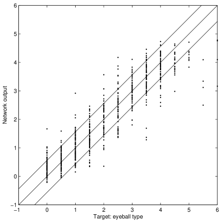
Figure 1: Median network type from ten runs versus eyeball morphological type for the eyeball test sample (683 galaxies), using all parameters and the 8:1 network architecture. The central diagonal line indicates the ideal result, i.e. assigned types equal to the known type; the diagonal lines above and below are the overall RMS deviation of the network types from the targets.

4.3.2 eClass Spectral Type

The ANNs are able to predict the eClass spectral type when trained on galaxies with spectra in the SDSS with a correlation of up to 0.95 and RMS of 0.06 (4 per cent) for the test sample in the range $-1$ to 0.5. The results for the simulation on the rest of DR1 are shown in Fig. 2. The shape is not perfect – a plot of net type - target type versus target type is not precisely symmetrical about zero, but the sigmoid shape seen when the training sample is not evenly sampled (§2) is not as pronounced. The sigmoid shape has been seen previously, e.g. Naim et al. (1995), where the network ‘avoided the ends of the scale’.

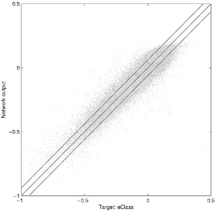
Figure 2: Median network type versus SDSS eClass spectral type for the simulation sample of 79,769 DR1 galaxies, using all parameters and the 8:1 network architecture. The diagonal lines show types equal and $\pm$ the RMS as in Fig. 1. Note that the RMS (0.060) and correlation (0.945) are not identical to those in Table 2, as this table shows results from the smaller test samples. However the difference is small.

4.3.3 Redshift

The generality of the method means that any parameter can be trained on and predicted, hence a photometric redshift can be obtained (Fig. 3). The correlation and RMS are up to 0.93 and down to 0.02. The RMS is comparable to other photometric redshifts in the literature found using neural networks, e.g. Tagliaferri et al. (2002) and Firth, Lahav & Somerville (2003), and to those derived from SDSS data (Csabai et al., 2003).

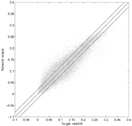
Figure 3: As Fig. 2, but with redshift as the target type (again 79,769 galaxies). For this simulation sample, the RMS is 0.020 and the correlation is 0.925.

5 Discussion

The main result is that the networks can predict morphological classifications, spectral types and redshifts of galaxies using just photometric parameters. This paper uses moderately sophisticated neural net techniques on a data set of unprecedented size and quality. There are many further techniques which could be used, and possibilities to try out. In particular there are many sophisticated ANN techniques which have been little used in astronomy but which may now be justified by the size of the datasets available. However, with the current data it is unlikely that they would make large improvements as the results are almost certainly limited by the intrinsic spread in the training samples, and one can never improve upon the training sample.

Possibilities include, at a basic level, varying the galaxy and neural net parameters used here, for example the number of random initializations or various Matlab parameters. More sophisticated neural net techniques include a better even sampling of the training sample so that targets are evenly spread over the range – here over-populated bins are simply cut down to size but under-populated bins are not altered. This may be especially useful for star formation rate and can be done using K-means clustering or a self-organising map (e.g. Tagliaferri et al., 2002). Improved regularisation, e.g. hierarchical Bayesian learning as opposed to weight decay, could be implemented. Multiple outputs for the network could be used to perform classification as opposed to regression. This is complementary work rather than an improvement and could be used for any of the types, in particular the eyeball types, or it could be used to e.g. assign probabilities to photometric redshift bins, as each output can give the a posteriori probability that the type is that output given its input parameters. This would also show objects for which the photometric redshift is less certain, as there may be no one bin with a high probability, or it may be split with peaks occurring in two separated bins. A different learning algorithm, e.g. quasi-Newton or conjugate gradient, would be needed for a classifier as Levenberg-Marquardt requires one output. Other learning algorithms could also be used with a validation sample. The disadvantage of a classifier is that the number of bins for the output is fixed for the network used. With the regression used here one can bin the assigned types afterwards if desired. Various methods exist for using committees of networks, apart from that here of using multiple random starts and using the median type assigned. Examples include constructive learning, bootstrap training samples, forward selection, backward elimination, cross validation and waterfall. There are other methods for global optimization apart from multiple random starts, e.g. simulated annealing and genetic algorithms. Many of these possibilities (regularisation, committees, etc.) are discussed at the comp.ai.neural-nets newsgroup FAQ at ftp://ftp.sas.com/pub/neural/index.html, whilst a waterfall of networks was used in galaxy classification by Adams & Woolley (1994). A further possibility is the use of unsupervised networks, i.e. those in which a predefined similarity criterion is used and the data is left to organize itself, with no training sample required. Unsupervised networks objectively find clusters of similar points in a dataset and can be used as a basis for classification. A well-known unsupervised network which has been used in classifying galaxies is the Kohonen self-organizing map (Kohonen, 2001), used by Naim et al. (1997b) for galaxy morphology. Naim et al. (1995) used principal component analysis to reduce a set of 24 galaxy parameters to 13 and found that the latter was as good for predicting types. This was tried, and found to be quicker for networks with more than  100 weights over ten runs but it was found that the correlations were generally slightly worse, as some information was lost (and it cannot be gained by PCA). The time taken was mainly that for the PCA, then the $N^{2}$ scaling for Levenberg-Marquardt with $N$ weights.

The usefulness of the methods here is that they are able to predict either spectral parameters using just photometry or assign morphological types at a vastly greater rate than humans but to the same accuracy. Much can be done with the types once they have been assigned, and this will form the basis of future work, in the distributions of these types and in their use to augment large scale structure studies using SDSS data with other physical measures such as colours.

The SDSS Southern Survey (York et al., 2000) is repeatedly imaging a smaller area of the southern galactic cap to go fainter in imaging and spectroscopy than the northern survey. Spectra from the Southern Survey could be used as training samples for galaxies at higher redshifts and below the northern spectroscopic flux limit.

One could thus look at galaxy evolution according to any assigned parameter. One could also, for example, project galaxies of unknown redshift about ones with known redshift, or push fainter down the luminosity function if assumptions are made about clustering. A particular statistic of interest is that of marked point processes (e.g. Beisbart, Kerscher & Mecke, 2002), in which the effects of intrinsic variation and those of environment can be separated.

Also, if one could predict physical parameters directly this would be extremely useful. One example is the star formation rate. The sample of 8,683 galaxies detailed in Gomez et al. (2003) was investigated. This is a volume limited sample from $0.05\leq z\leq 0.095$ with well measured redshifts and H$\alpha$ star formation rate. At present the star formation rate is poorly predicted by the ANN, being best at zero but widely spread above this. Improved results may be obtained for networks trained on just those galaxies which are star forming.

Further targets which could be predicted include the bulge to disc ratio or the 2dF $\eta$ spectral type, and there are further galaxy parameters which could be used such as Sérsic indices, or spectral parameters for predicting morphological types.

It is not immediately obvious whether the resulting distributions say more about the galaxies or the assigned types, but with the numbers of galaxies available biases in the assigned types from the network could be studied in detail. Any biases of this sort are already less than the intrinsic spread in assigned type and one could compare results using a sample where the target types are available to see if different results are obtained. If not, then as long as the sample used has photometry of which the training sample was representative, the network types can be used with confidence.

6 Conclusions

The neural nets are able to predict the eyeball morphological type, the spectral type eClass, and the redshift using parameters available for all galaxy images in the Sloan Digital Sky Survey Data Release One. The correlations are 0.93, 0.95, and 0.93 respectively. The mean RMS errors between the network output and the known type for a set of unseen galaxies of which the training set formed a representative part are 0.55, 0.06 and 0.02 (approximately 9, 4, and 5 per cent of the ranges of the targets).

References

- Abazajian et al. (2003) Abazajian K., et al., 2003, preprint (astro-ph/0305492)
- Adams & Woolley (1994) Adams A., Woolley A., 1994, Vistas in Astronomy, 38, 273
- Ball (2001) Ball N. M., 2001, MSc Thesis, University of Sussex
- Bazell & Aha (2001) Bazell D., Aha D. W., 2001, ApJ, 548, 219
- Bazell (2000) Bazell D., 2000, MNRAS, 316, 519
- Beisbart et al. (2002) Beisbart C., Kerscher M., Mecke K., 2002, in Mecke K., Stoyan D., eds, Lecture Notes in Physics, vol. 600, Morphology of Condensed Matter. Springer-Verlag, Heidelberg, p. 358
- Bishop (1995) Bishop C. M., 1995, Neural Networks for Pattern Recognition, Oxford University Press, Oxford
- Cohen et al. (2003) Cohen S. H., Windhorst R. A., Odewahn S. C., Chiarenza C. A., Driver S. P., 2003, AJ, 125, 1762
- Connolly et al. (1995) Connolly A. J., Szalay A. S., Bershady M. A., Kinney A. L., Calzetti D., 1995, AJ, 110, 1071
- Connolly & Szalay (1999) Connolly A. J., Szalay A. S., 1999, AJ, 117, 2052
- Csabai et al. (2003) Csabai I., Budavári T., Connolly A. J., et al., 2003, AJ, 125, 580
- de Theije & Katgert (1999) de Theije P. A. M., Katgert P., 1999, A&A, 341, 371
- de Vaucouleurs (1948) de Vaucouleurs G., 1948, Annales d’Astrophysique, 11, 247
- de Vaucouleurs (1959) de Vaucouleurs G., 1959, Handbuch der Physik, 53, 275
- Eisenstein et al. (2001) Eisenstein D. J., Annis J., Gunn J. E., et al., 2001, AJ, 122, 2267
- Firth et al. (2003) Firth A. E., Lahav O., Somerville R. S., 2003, MNRAS, 339, 1195
- Folkes et al. (1996) Folkes S. R., Lahav O., Maddox S. J., 1996, MNRAS, 283, 651
- Freeman (1970) Freeman K. C., 1970, ApJ, 160, 811
- Fukugita et al. (1996) Fukugita M., Ichikawa T., Gunn J. E., Doi M., Shimasaku K., Schneider D. P., 1996, AJ, 111, 1748
- Goderya & Lolling (2002) Goderya S. N., Lolling S. M., 2002, Ap&SS, 279, 377
- Gomez et al. (2003) Gomez P. L., Nichol R. C., Miller C. J., et al., 2003, ApJ, 584, 210
- Gunn et al. (1998) Gunn J. E., Carr M., Rockosi C., et al., 1998, AJ, 116, 3040
- Hogg et al. (2001) Hogg D. W., Finkbeiner D. P., Schlegel D. J., Gunn J. E., 2001, AJ, 122, 2129
- Kohonen (2001) Kohonen T., 2001, Self-Organizing Maps, 3rd extended edition, Springer Series in Information Sciences, Vol. 30, Springer, Berlin
- Lahav et al. (1995) Lahav O., Naim A., Buta R. J., et al., 1995, Sci, 267, 859
- Lahav et al. (1996) Lahav O., Naim A., Sodré L., Storrie-Lombardi M. C., 1996, MNRAS, 283, 207
- Levenberg (1944) Levenberg, K., 1944, Quarterly Journal of Applied Mathematics II (2), 164
- Lupton et al. (1999) Lupton R. H., Gunn J. E., Szalay A. S., 1999, AJ, 118, 1406
- Lupton et al. (2001) Lupton R. H., Gunn J. E., Ivezić Z., Knapp G. R., Kent S., Yasuda N., 2001, in ASP Conf. Ser. 238, Astronomical Data Analysis Software and Systems X, ed. F. R. Harnden, Jr., F. A. Primini, and H. E. Payne (San Francisco: Astr. Spc. Pac.) (astro-ph/0101420)
- Madgwick et al. (2002) Madgwick D. S., Lahav O., Baldry I. K., et al., 2002, MNRAS, 333, 133
- Madgwick (2003) Madgwick D. S., 2003, MNRAS, 338, 197
- Marquardt (1963) Marquardt, D.W., 1963, Journal of the Society of Industrial and Applied Mathematics 11 (2), 431-441.
- Molinari & Smareglia (1998) Molinari E., Smareglia R., 1998, A&A, 330, 447
- Naim et al. (1995) Naim A., Lahav O., Sodre L., Storrie-Lombardi M. C., 1995, MNRAS, 275, 567
- Naim et al. (1997) Naim A., Ratnatunga K. U., Griffiths R. E., 1997a, ApJ, 476, 510
- Naim et al. (1997b) Naim A., Ratnatunga K. U., Griffiths R. E., 1997b, ApJS, 111, 357
- Nakamura et al. (2003) Nakamura O., Fukugita M., Yasuda N., Loveday J., Brinkmann J., Schneider D. P., Shimasaku K., SubbaRao M., 2003, AJ, 125, 1682
- Odewahn et al. (1996) Odewahn S. C., Windhorst R. A., Driver S. P., Keel W. C., 1996, ApJL, 472, L13
- Odewahn et al. (2002) Odewahn S. C., Cohen S. H., Windhorst R. A., Philip N. S., 2002, ApJ, 568, 539
- Parker (1985) Parker D. B., 1985, Report TR-47. MIT, Center for Computational Research in Economics and Management Science, Cambridge, MA
- Petrosian (1976) Petrosian V., 1976, ApJL, 209, L1
- Pier et al. (2003) Pier J. R., Munn J. A., Hindsley R. B., Hennessy G. S., Kent S. M., Lupton R. H., Ivezić Ž., 2003, AJ, 125, 1559
- Pogson (1856) Pogson N., 1856, MNRAS, 17, 12
- Rumelhart et al. (1986) Rumelhart D. E., Hinton G. E., Williams R.J., 1986, Nat, 323, 533
- Schlegel et al. (1998) Schlegel D. J., Finkbeiner D. P., Davis M., 1998, ApJ, 500, 525
- Serra-Ricart et al. (1993) Serra-Ricart M., Calbet X., Garrido L., Gaitan V., 1993, AJ, 106, 1685
- Slonim et al. (2001) Slonim N., Somerville R., Tishby N., Lahav O., 2001, MNRAS, 323, 270
- Smith et al. (2002) Smith J. A., Tucker D. L., Kent S., et al., 2002, AJ, 123, 2121
- Storrie-Lombardi et al. (1992) Storrie-Lombardi M. C., Lahav O., Sodre L., Storrie-Lombardi L. J., 1992, MNRAS, 259, 8p
- Stoughton et al. (2002) Stoughton C., Lupton R. H., Bernardi M., et al., 2002, AJ, 123, 485
- Strauss et al. (2002) Strauss M. A., Weinberg D. H., Lupton R. H., et al., 2002, AJ, 124, 1810
- Tagliaferri et al. (2002) Tagliaferri R., Longo G., Andreon S., Capozziello S., Donalek C., Giordano G., 2002, preprint (astro-ph/0203445)
- Werbos (1974) Werbos P. J., 1974, PhD thesis, Harvard Univ., Cambridge, MA
- Windhorst et al. (1999) Windhorst R., Odewahn S., Burg C., Cohen S., Waddington I., 1999, Ap&SS, 269, 243
- Yip et al. (2002) Yip C. W., Connolly A. J., Szalay A., et al., 2002, SDSS publication no. 202
- York et al. (2000) York D. G., Adelman J., Anderson J. E., et al., 2000, AJ, 120, 1579