The Munich Near-Infrared Cluster Survey (MUNICS) – II. The $K$-band luminosity function of field galaxies to $z~{}\sim~{}1.2$

Abstract

We present a measurement of the evolution of the rest-frame $K$-band luminosity function to $z\sim 1.2$ using a sample of more than 5000 $K$-selected galaxies drawn from the MUNICS dataset. Distances and absolute $K$-band magnitudes are derived using photometric redshifts from spectral energy distribution fits to BVRIJK photometry. These are calibrated using $>500$ spectroscopic redshifts. We obtain redshift estimates having a rms scatter of $0.055$ and no mean bias. We use Monte-Carlo simulations to investigate the influence of the errors in distance associated with photometric redshifts on our ability to reconstruct the shape of the luminosity function. Finally, we construct the rest-frame $K$-band LF in four redshift bins spanning $0.4<z<1.2$ and compare our results to the local luminosity function. We discuss and apply two different estimators to derive likely values for the evolution of the number density, $\Phi^{*}$, and characteristic luminosity, $M^{*}$, with redshift. While the first estimator relies on the value of the luminosity function binned in magnitude and redshift, the second estimator uses the individually measured $\{M,z\}$ pairs alone. In both cases we obtain a mild decrease in number density by $\sim 25\%$ to $z=1$ accompanied by brightening of the galaxy population by $0.5$ to $0.7$ mag. These results are fully consistent with an analogous analysis using only the spectroscopic MUNICS sample. The total $K$-band luminosity density is found to scale as $d\log\rho_{L}/dz=0.24$. We discuss possible sources of systematic errors and their influence on our parameter estimates. By comparing the luminosity density and the cumulative redshift distributions of galaxies in single survey fields to the sample averages, we show that cosmic variance is likely to significantly influence infrared selected samples on scales of $\sim 100$ square arc minutes.

1 Introduction

The luminosity function (LF) is the most basic statistic used to study galaxy populations and their evolution. Its dependence on wavelength and look-back time provides important constraints on the evolution of the global properties of the galaxy population.

Recently, progress in measuring the optical galaxy LF was made both locally and at higher redshift. Locally, results from the 2dF survey (Folkes et al., 1999; Madgwick et al., 2002) and 2MASS (Kochanek et al., 2001) provide much improved measurements of the LF as a function of galaxy morphology, environment, and wavelength. In spite of some controversy regarding the normalization and the very faint end slope of the local LF, it is a well established result that the LF depends on galaxy type, although the correlations are not always very tight. Generally, the faint end is populated by galaxies of smaller mass, later morphology, bluer colors and later spectral type, and stronger line emission. The bright end is dominated by early-type spirals and ellipticals, and the very bright end by giant ellipticals (e.g. Marzke et al., 1994; Bromley et al., 1998; Madgwick et al., 2002).

A number of studies of the luminosity function of galaxies at $0\lesssim z\lesssim 1$ using optically selected redshift surveys have been published in recent years (e.g. Efstathiou et al., 1988; Lilly et al., 1995b; Heyl et al., 1997; Lin et al., 1997; Liu et al., 1998; Ratcliffe et al., 1998; Lin et al., 1999). These surveys (with samples of typically hundreds of objects) have consistently found similar trends in the evolution of the rest-frame $B$-band field galaxy LF. The main result was the contrast between the rapid evolution of the blue, star-forming sub-population and the mild change in the redder, early-type population. Simultaneously, first results at $z\sim 3$ became available through the study of Lyman-break galaxies (Shapley et al., 2001).

The ground-breaking CFRS (Lilly et al., 1995a) found that the luminosity function in the rest-frame $B$-band of the blue field population brightens by roughly 1 mag to $z\simeq 1$ and also becomes steeper at the faint end at $z\gtrsim 0.5$ (see also Heyl et al., 1997). In contrast, the red population was found to show very little change in either number density or luminosity (Lilly et al., 1995b). Lin et al. (1999) attempted to discriminate explicitly between number-density and luminosity evolution in the CNOC2 sample consisting of roughly 2000 galaxies. They found that the early-type population shows positive luminosity evolution (1.6 mag) which is nearly compensated by negative density evolution (factor of 0.5), so that there is little net change in their overall LF. The intermediate-type population shows positive luminosity evolution (0.9 mag) plus weak positive density evolution (factor of 1.7), resulting in mild positive evolution in its luminosity density. The amount of luminosity evolution in the early-type and intermediate-type populations was found to be consistent with expectations from models of passive evolution of their stellar populations. In contrast, the late-type population is best fit by a strong increase in number density at high redshift (factor of 4.1), accompanied by only little positive luminosity evolution (0.2 mag). The overall $B$-band luminosity density of late-type objects was found to increase rapidly in both the CFRS and CNOC2 samples, while the luminosity density of early-type objects was found to be nearly constant.

In contrast to the blue and optical wave-bands, the near infrared $K$-band light of galaxies is much less affected by dust, much less sensitive to ongoing star-formation and much less dependent on galaxy type. Furthermore, the near-IR luminosity is as a reasonable tracer of the stellar mass of a galaxy, since the near-IR light is dominated by the light of old and evolved stars. Therefore, by investigating the $K$-band properties of galaxies as a function of redshift, we may hope to be able to move from a picture dominated by the evolution of star formation to one which focuses on the assembly history of mass in these systems – one of the most fundamental predictions of cold dark matter based structure formation theories.

Most near-IR selected surveys so far have been either small in size or shallow (e.g. Glazebrook et al., 1995; Gardner et al., 1997; Cowie et al., 1996; Szokoly et al., 1998). Furthermore, optical followup spectroscopy of near-IR selected samples to $z\sim 1$ is difficult because of the large range of optical to near-IR (e.g. $R\!-\!K$) colors of galaxies, although spectroscopic samples of a few hundred objects are now available (Feulner et al., 2003; Pozzetti et al., 2003; Cimatti et al., 2002). If any change in the LF was seen at all, only mild luminosity evolution at $z>0.5$ has been significantly detected.

In this work, we aim at measuring the rest-frame $K$-band luminosity function of galaxies and its evolution with redshift in the range $0.4<z<1.2$ using the $K$-band selected, BVRIJK multicolor data set of the MUNICS project (Drory et al., 2001b). The sample contains more than 5000 objects and covers a large solid angle. We use spectroscopically calibrated photometric redshifts (using more than 500 spectroscopic redshifts) to estimate distances and spectral energy distribution (SED) fitting techniques to extrapolate the SED to rest-frame $K$.

This paper is organized as follows. First, we briefly introduce the galaxy sample we use in this work in Sect. 2. Next, in Sect. 3, we describe the photometric redshift estimation technique along with the construction of a set of semi-empirical SEDs best matching the SEDs present in the sample. In Sect. 4 we discuss the construction of the rest-frame $K$-band luminosity function from photometric redshifts and assess the influence of errors in $z$ by means of Monte-Carlo simulations. The resulting luminosity function is presented in Sect. 5, and its evolution is investigated in Sect. 6. Sect. 7 discusses the results and Sect. 8 summarizes this work.

We assume $\Omega_{\rm M}=0.3$, $\Omega_{\Lambda}=0.7$ throughout this paper. We write Hubble’s Constant as $H_{0}=100\ h\ \mathrm{km\ s^{-1}\ Mpc^{-1}}$, using $h=0.65$ unless the quantities in question can be written in a form explicitly depending on $h$.

2 The galaxy sample

MUNICS is a wide-area, medium-deep, photometric and spectroscopic survey selected in the $K$ band, reaching $K\sim 19.5$. It covers an area of roughly one square degree in the $K$ and $J$ bands with optical follow-up imaging in the $I$, $R$, $V$, and $B$ bands in 0.4 square degrees. Drory et al. (2001b, hereafter MUNICS I) discusses the field selection, object extraction and photometry in the $K,J,I,R$, and $V$ bands. The $B$ band imaging was completed more recently and the data were processed in an analogous way as described in MUNICS I. Detection biases, completeness, and photometric biases of the MUNICS data are analyzed in detail in Snigula et al. (2002, hereafter MUNICS IV).

The MUNICS photometric survey is complemented by spectroscopic follow-up observations of all galaxies down to $K\leq 17.5$ in 0.25 square degrees, and a sparsely selected deeper sample down to $K\leq 19$. It contains more than 550 secured redshifts. The spectra cover a wide wavelength range of $4000-8500$Å at $13.2$Å resolution, and sample galaxies at $0<z<1$. These observations are described in detail in Feulner et al. (2003, hereafter MUNICS V).

The galaxy sample used in this work is a subsample of the MUNICS survey Mosaic Fields (see MUNICS I), selected for best photometric homogeneity, good seeing, and similar depth. Furthermore, in each of the survey patches, areas close to the image borders in any passband, areas around bright stars, and regions suffering from blooming are excluded. The subsample covers 0.28 square degrees in $B$, $V$, $R$, $I$, $J$, and $K$. Table 1 lists the Mosaic Fields used in the subsequent analysis. It is almost identical to the sample used in Drory et al. (2001a, hereafter MUNICS III), except for the additional $B$-band imaging data (and hence refined photometric redshifts).

Stars are identified following the procedure described in MUNICS I, adding a color criterion in the $J\!-\!K$ vs. $V\!-\!I$ plane to exclude faint stellar sources which cannot be separated from galaxies morphologically (see Fig. 10 in MUNICS I). This color criterion may also exclude $z\lesssim 0.2$ compact blue galaxies. Such galaxies are very unlikely to be present in the $K$-selected sample, given our magnitude limit. We will restrict our analysis of the luminosity function to $z>0.4$ such that this is anyway not a problem.

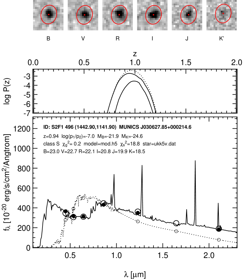
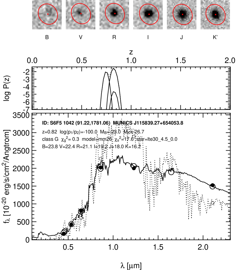
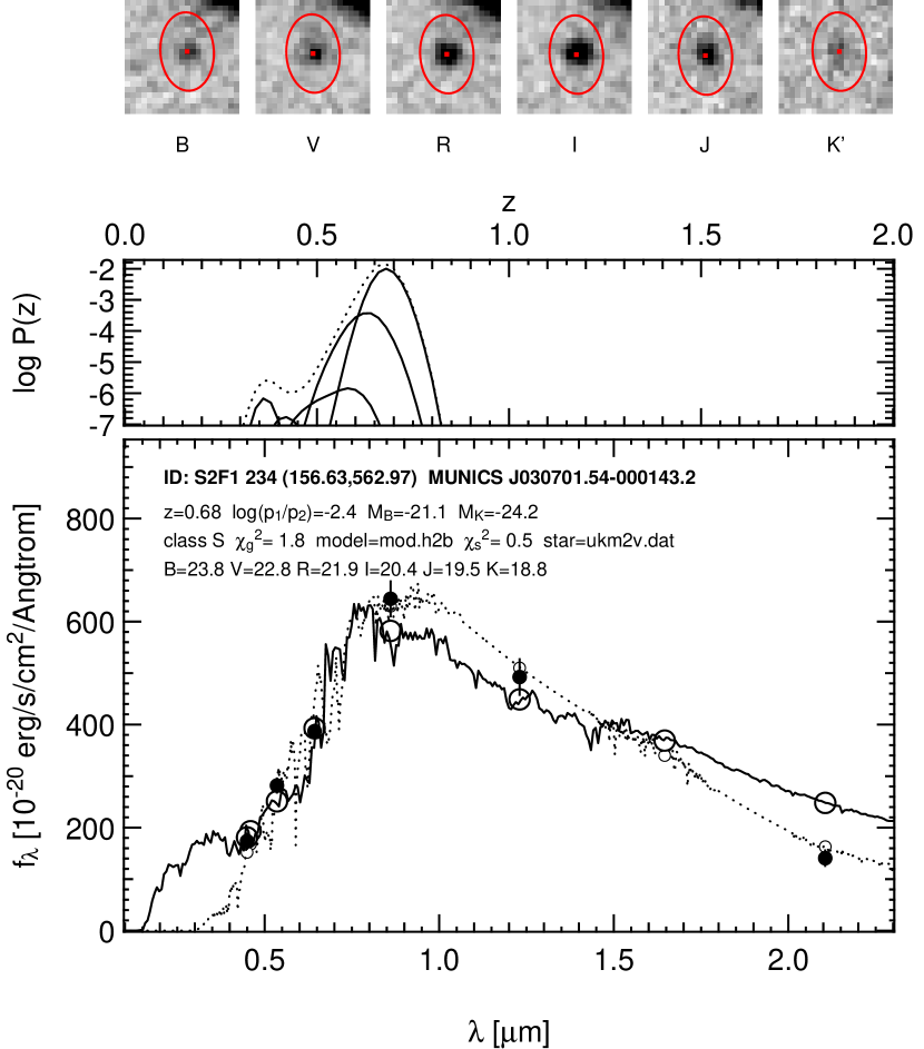
Figure 5: Examples of the determination of photometric redshifts. The implications of these examples are discussed in the text. The lower panels show the best-fitting galaxy SED (solid line), the best-fitting stellar SED (dotted line), the expected fluxes in observed-frame $B$,$V$,$R$,$I$,$J$, and $K$ (open circles) and the measured fluxes (filled circles). The middle panel shows the redshift probability function for the different galaxy template SEDs and the total redshift probability function. The upper panels show thumbnail images of the objects in our six pass bands.

To make sure that our star-galaxy separation does not cause any systematic biases in our analysis, we double check the method by including stellar SEDs in the template library used to estimate photometric redshifts (see below). We find that the objects identified as stars are indeed better fit by a pure stellar SED than by any galactic SED (see right panel in Fig. 5). Most exceptions (a few percent of the stars) are most probably binaries. Using only the SED fit to discriminate stars from galaxies does not change any of the results of this work.

3 Photometric redshifts

Photometric redshifts are derived using the method presented in Bender et al. (2001) and Bender (2003). We only briefly outline the procedure in this section. The method is a template matching algorithm rooted in Bayesian statistics closely resembling the method presented by Benítez (2000). However, instead of relying on a predetermined set of template SEDs, semi-empirical templates matching the photometric properties of the sample are used. The templates are derived by fitting stellar population models of Maraston (1998) of different age and dust extinction and Kinney-Calzetti (Kinney et al., 1996) spectra to combined broad-band energy distributions of MUNICS and FDF (Heidt et al., 2003) galaxies having spectroscopic redshifts. In this way, representative galaxy templates of mixed stellar populations (variable age, metallicity, and dust extinction) optimized for the MUNICS dataset are obtained.

The total spectroscopic sample is divided into 2 groups of objects. The first subsample (all objects with redshifts in the field S2F1) is used for constructing SED templates, the second subsample (all other objects with spectroscopic redshifts) is used for comparing spectroscopic and photometric redshifts and thereby calibrating the SED library.

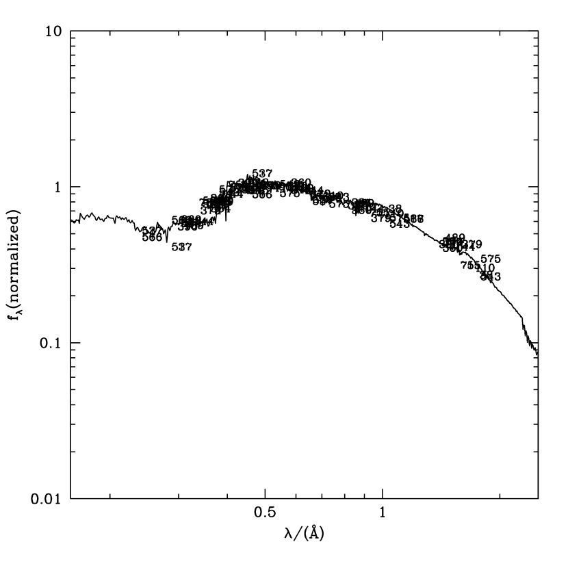
Figure 1: A low-resolution spectrum constructed from BVRIJK photometry of objects with known spectroscopic redshifts. The objects’ photometry is de-redshifted to $z=0$ and normalized to a common magnitude and fit by stellar population synthesis models. Objects best fitting the same model are grouped together and used in an iterative procedure to find an optimal set of SEDs to use as templates. The measured fluxes of each object are marked by the object’s ID. The solid line is the final SED template which best fits this class of objects.

The observed-frame apparent magnitudes of objects in the first subsample are transformed to rest-frame redshift zero, and fitted by an initial set of stellar population synthesis models. Objects best fitting the same model are grouped together. Since each group will contain objects from a variety of redshifts, a densly sampled SED from the broad band photometry of these objects is obtained. This procedure is illustrated in Fig. 1.

This initial set of SEDs is used to determine photometric redshifts for the total sample of objects having spectroscopic redshifts. The photometric redshifts are compared to the spectroscopic ones, and, additionally, the same de-redshifting procedure is applied to the spectroscopic sub-sample not used for the initial construction of the SEDs, only that now we group the objects by the SED that gave the best fit during the determination of the photometric redshift. Using this comparison, deficiencies in the set of SEDs can be identified as those become apparent through systematic offsets between the de-redshifted magnitudes and the SED templates. This is the case since such deficiencies lead to a wrongly determined photometric redshift and therefore to the assignment of a wrong SED.

This procedure is repeated with a refined set of SEDs, by changing SEDs, abolishing some and adding others, until a satisfactory library of template SEDs is found. Fig. 2 shows the final template SED library used to derive photometric redshifts in what follows.

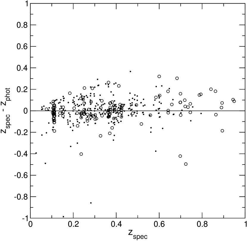
Figure 3: The difference between spectroscopic and photometric redshift vs. spectroscopic redshift for the subsample used to construct the SED templates (open circles) and all other objects (filled circles).

In Fig. 3 we plot the difference between spectroscopic and photometric redshift vs. spectroscopic redshift for the subsample used to construct the SED templates and for the rest of the sample which was used to test the procedure. There is no apparent difference between these two error distributions.

Finally, Fig. 4 compares photometric and spectroscopic redshifts for all $\sim 500$ objects within five MUNICS Mosaic Fields and shows the distribution of redshift errors. The typical scatter in the relative redshift error $\Delta z/(1+z)$ is 0.055. The mean redshift bias is negligible. The distribution of the errors is roughly Gaussian. There is no visible difference between the distributions among the survey fields. Although this performance is encouraging, it is important to say that the spectroscopic data become sparse at $z\gtrsim 0.6$ and there are only two spectroscopic redshifts at $z>1$.

To illustrate the use of photometric redshifts, we show two instructive examples of photometric redshift determinations of galaxies and the identification of an M-star in Fig. 5. These examples help to understand how the technique works and the uncertainties involved.

Firstly, a spiral-like system at redshift around unity. Here the Balmer break is redshifted beyond the $R$-band filter, and only one SED contributes significantly to the global peak in the redshift probability distribution. The rather broad probability distribution in redshift is due to the fact that the Balmer break is in the rather large sampling gap between the $R$ and $I$ bands, and therefore its position is not very well determined. Note that this object, although very bright in the optical, is very faint in the $K$ band, and therefore probably a rather low-mass system.

Secondly, an early-type object at redshift $z\sim 0.82$. The redshift determination can be regarded as quite secure although there are competing SEDs around the global peak of the redshift probability function. In this case, the redshift is determined by the 4000Å break and the steep decline in flux bluer thereof. Because the object is undetected in $B$ and only barely detected in $V$, the rest-frame UV and blue slopes of the spectrum are not firmly determined and hence slightly differing effective ages are giving reasonable fits. This uncertainty in age or type translates into an uncertainty in redshift. Therefore there are competing SEDs at similar but not identical redshifts contributing to the total redshift probability distribution.

Common to both above examples is that the position in redshift of the global maximum of the total redshift probability distribution is always compatible with the redshift one would derive by looking at the probability distribution of the most likely SED.

The third panel in Fig. 5 shows an object best fit by the SED of an M2 star. We have used a criterion based on a comparison of the best $\chi^{2}$ for redshifted galaxy template SEDs and stellar SEDs to discriminate between star and galaxies, to test the robustness of the morphological and color based star-galaxy separation presented in MUNICS I, hoping to be able to improve the procedure at faint magnitudes. The main problem hereby is the lack of reliable SEDs for cool stars with the necessary broad wavelength coverage. Using only this SED based star-galaxy separation instead of the morphological method does not change the results of this work. Note that we present an independent measure of the reliability of our star-galaxy separation in MUNICS V, where we test it against blind spectroscopy.

It is interesting to compare the photometric redshifts obtained using the present six-color photometry to the ones used in MUNICS III, where we did not have B-band imaging yet and the spectroscopic calibration sample was smaller (310 objects as opposed to 550 now). This comparison is shown in Fig.6. In spite of overall reasonable agreement, there are some important differences. The most notable one is that objects tend to scatter to lower redshifts if $B$-band photometry is missing. Objects are scattered preferably to the region in redshift below which the 4000Å break enters the observed filter set (because this peak in the $z$-probability function cannot be excluded by the missing blue photometry). Another set of objects is redistributed from $z\sim 1.2$ (six-colors) to lower redshifts (five-colors). These objects all have blue colors and rather late type SEDs. Both effects are small in numbers, affecting $\sim 3$ per cent of the sample. Therefore they do not show up in the spectroscopic calibration and are difficult to eliminate systematically. The influence of such an effect on the luminosity function can be significant although the number of affected objects is small if rare high-luminosity objects are preferably affected. This is discussed below in Sect. 5.

In Fig. 7 we plot absolute $K$-band magnitude vs. photometric redshift and the redshift distribution of the total sample discussed here, containing 5132 galaxies. The redshift distribution peaks around $z\approx 0.5$ and has a tail extending to $z\approx 3$. An analytical fit of the form

$$\frac{dN}{dz}\;=\;\frac{\beta z^{2}}{\Gamma(3/\beta)\>z_{0}^{3}}\>e^{-(z/z_{0})^{\beta}}$$ (1)

is also shown. The best-fitting values are $z_{0}=0.101,\beta=0.746$.

Finally, we plot the cumulative redshift distribution of bright galaxies in the $K$-band in Fig. 8. We select galaxies with apparent $K$-band magnitudes in the interval $16<m_{K}<18$, where the present sample is definitively complete. The figure also compares the data in the single survey fields to the sample average. We find that cosmic variance is significant on scales of $\sim 100$ square arc minutes, the typical size of previous infrared selected surveys.

4 Computing the luminosity function

4.1 The $V_{\mathrm{max}}$ method

We estimate the luminosity function, $\Phi(M)dM$, the comoving number density of galaxies with absolute magnitude in the range $[M,M+dM)$, using the $V_{\mathrm{max}}$ formalism (Schmidt, 1968) to account for the fact that some fainter galaxies are not visible in the whole survey volume.

Each galaxy in a given redshift bin $[z_{l},z_{h})$ contributes to the number density an amount inversely proportional to the volume in which the galaxy is detectable in the redshift bin given all relevant observational constraints:

$$V_{i}\;=\;d\Omega\,\int_{z_{l}}^{\mathrm{min}(z_{h},z_{max})}\,\frac{dV}{dz}\,dz,$$ (2)

where $dV/dz$ is the comoving volume element, $d\Omega$ is the survey area, $z_{max}$ is the maximum redshift at which galaxy $i$ having absolute magnitude $M_{K,i}$ is still detectable given the limiting apparent magnitude of the survey and the galaxy’s SED (the best-fit SED from the photometric redshift determination in our case).

Additionally, the contribution of each galaxy $i$ is weighted by the inverse of the detection probability, $P(m_{K,i})$, where we assume that the detection probability is independent of the galaxy type and can be approximated by that of point-like sources. We only include objects with $P(m_{K,i})>0.75$, such that this correction is always small. We have checked that this correction does not bias our results by comparing to what we get for higher completeness limits. Also, the results of completeness simulations discussed in MUNICS IV demonstrate that although there exist profile-dependent surface-brightness selection biases, these are under control for redshifts up to $z\gtrsim 1$, and that the onset of incompleteness is roughly independent of profile type.

The comoving number density of objects in a given absolute magnitude interval and redshift bin is finally calculated as

$$\Phi(M)dM=\sum_{i}\frac{1}{V_{\mathrm{max}}^{i}}\frac{1}{P(m_{K,i})}dM,$$ (3)

where the sum is to be taken over all objects $i$ in the bin.

The advantage of the $V_{\mathrm{max}}$ method is that it is non-parametric, i.e. no assumption on the form of the LF is made and the estimate of the LF in each redshift and magnitude bin is independent. There is no need to compute the normalization of the LF separately. It is quick and easy to compute. The major disadvantage is that this method is sensitive to clustering in the sample. In our case we might hope that this is not a major concern since we average over a large volume and probe multiple independent lines of sight.

Takeuchi et al. (2000) performed a systematic comparison of different estimators for the luminosity function, finding that the $V_{\mathrm{max}}$ estimator yields a completely unbiased result if there is no inhomogeneity. Earlier claims that the $V_{\mathrm{max}}$ estimator is biased even without clustering were not confirmed. The $V_{\mathrm{max}}$ estimator was also found to give consistent results with other statistical estimators analyzed, despite of its sensitivity on large scale structure.

The last missing ingredient is the absolute $K$-band magnitude. It is computed by extrapolation from the observed-frame colors, using the best-fit SED from the photometric redshift code. The near-IR slopes of the SEDs are fairly uniform across galaxy types (the $K$-band $k$-corrections are small and almost type-independent) and so the uncertainty introduced by this extrapolation is rather small, of the order of $\Delta M_{K}\sim 0.1$ mag in the mean, and thus small compared with the uncertainty of the total rest-frame $K$-band magnitude coming from the uncertainty in the distance.

4.2 Monte-Carlo simulations

The use of photometric redshifts, in general, can introduce systematic errors in the derived galaxy distances and therefore in the luminosity function which we want to derive in what follows. Therefore, we perform Monte-Carlo simulations to test the robustness of the LF estimate under the conditions imposed by the use of photometric redshifts instead of spectroscopic distances. We generate mock MUNICS-like catalogs following a non-evolving LF and compare the output of the LF estimate as described above with the input LF. Note that we can only test the effects of random errors in the distances and not the influence of systematically wrong distances as those shown in Fig. 6.

The simulated LF follows the form of th local 2MASS $K$-band LF of Kochanek et al. (2001). We assume that there is no redshift evolution in brightness or number density. The extrapolation of the flux to the rest-frame $K$-band was done using the mean $k$-correction of the models used for determining photometric redshifts (Fig. 2).

To investigate the influence that errors in the photometric redshifts have on recovering the form of the LF, we simulate four data sets with errors $\Delta z$ drawn from a Gaussian of width $0.02$, $0.055$ (the value found from the comparison with spectroscopic redshifts in Fig. 4), $0.1$, and $0.2$. The simulations are repeated 10 times, and the LF is extracted in four redshift bins, $0.4<z<0.6,0.6<z<0.8,0.8<z<1.0,$ and $1.0<z<1.2$. The results are shown in Fig. 9.

The overall impression from Fig. 9 is that the form is well reproduced, and that, as expected, the influence of the redshift uncertainty is larger at small redshifts where the relative influence on the distance is largest. The form of the LF only becomes significantly biased when the redshift errors exceed $\Delta z\gtrsim 0.1$, becoming a significant fraction of the redshift bin size. There, the well-known effect of objects being preferably scattered away from $L^{*}$, producing too many bright objects and too few lower luminosity objects becomes apparent. For the value $\Delta z=0.055$ (upper right panel in Fig. 9), the form is only slightly affected in the lowest redshift bin, $0.4<z<0.6$.

From the last said we conclude that the shape of the luminosity function is not significantly biased as long as the photometric redshifts scatter symmetrically around the true redshifts (see also Subbarao et al., 1996) and their errors are (significantly) smaller than the bin size in $z$ over which the luminosity function is averaged.

4.3 Influence of the incompleteness corrections

The corrections for incompleteness involve the volume correction, $1/V_{\mathrm{max}}$, and the correction for the detection incompleteness at fainter magnitudes, $1/P(m_{K,i})$.

Given our magnitude limits, both corrections do not play any role at magnitudes brighter than $M_{K}^{*}\approx-23.5$. At fainter magnitudes both corrections contribute significantly. The $V_{\mathrm{max}}$ term becomes dominant at the faintest levels (as we exclude objects with $P(m_{K,i})<0.75$).

In the lowest redshift bin the $V_{\mathrm{max}}$ term is ill-determined resulting in a steepening in the LF’s very faint end. The reason is the redshift error associated with photometric redshifts and that the approximation of the visibility function as that of a point source breaks down at low redshifts where the objects are well-resolved. The steepening at of the LF can be explained in terms of low luminosity galaxies having true redshifts just lower than the bin’s lower bound, which are scattered upwards in $z$ by the photometric redshift estimate and just make it into the bin. As those galaxies are close to the detection limit, the $V_{\mathrm{max}}$ test predicts them to be detectable only in a very small volume of the bin and therefore the $V_{\mathrm{max}}$ correction becomes large (factors of 5 and above), producing the observed behavior. Therefore our data do not allow us to place constraints on the faint end slope of the LF, even in our lowest redshift bin.

5 Results

In this section we present the results on the evolution of the rest-frame $K$-band luminosity function to $z\leq 1.2$.

In Fig. 10 we plot the rest-frame $K$-band luminosity function obtained from the present MUNICS dataset. The plot shows the uncorrected values as well as the $V_{\mathrm{max}}$ and incompleteness corrected ones. For comparison, we also show the local $z=0$ 2MASS $K$-band LF (Kochanek et al., 2001) and a Schechter function evolved with $z$ using the best-fit values for the evolution parameters $\mu=1/\Phi^{*}(0)d\Phi^{*}/dz$ and $\nu=dM^{*}/dz$ from Sect. 6. Note that these are not independent Schechter fits in each redshift bin but rather a global estimate of the change in $\Phi^{*}$ and $L^{*}$ with redshift (see below).

Taken at face value, it is apparent that the total rest-frame $K$-band LF evolves only mildly to $z=1.2$. This is in qualitative agreement with the finding of Cowie et al. (1996) from a much smaller spectroscopic sample, where the authors found that the $K$-band LF in the redshift bin $0.6<z<1$ was consistent with the one at $0<z<0.2$ (using an Einstein-de-Sitter cosmology).

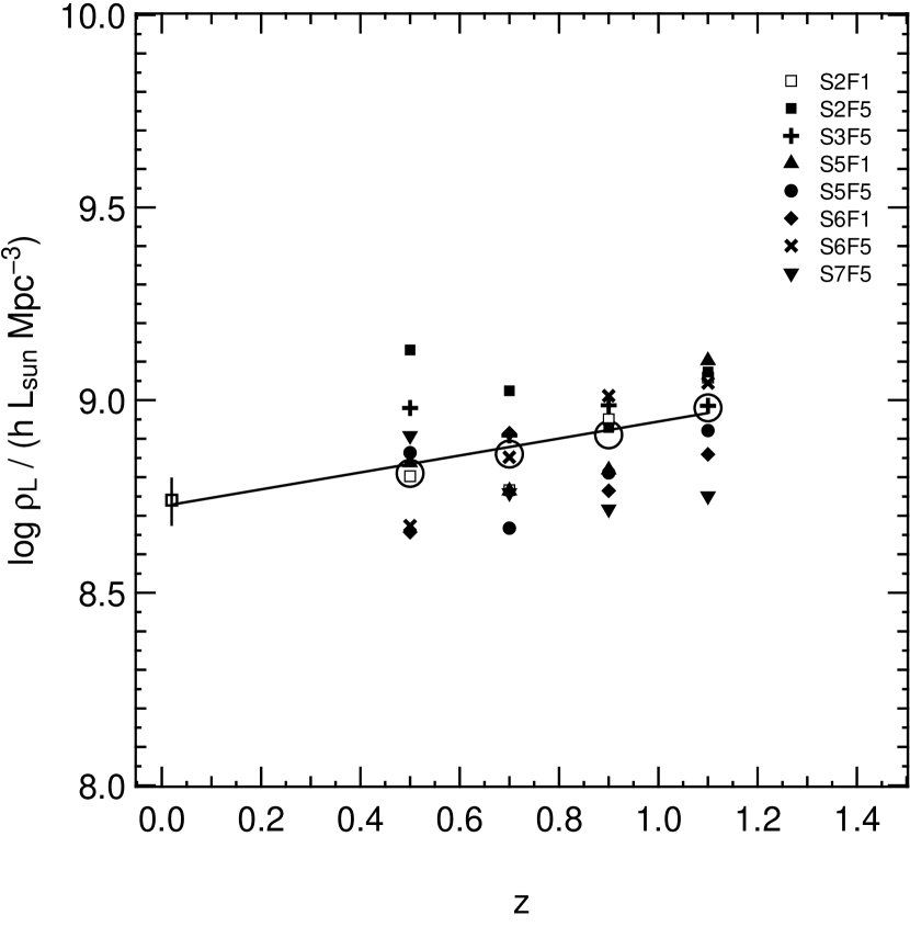
Figure 11: The rest-frame $K$-band luminosity density at $0.4<z1.2$. Different symbols denote the different survey patches (Mosaic Fields). The large open circles are average values. The point at $z=0.02$ is taken from Kochanek et al. (2001). The solid line represents the expected total luminosity density using the best-fit values for the evolution parameters $\mu=-0.25$ and $\nu=-0.53$ from Sect. 6.

This is further demonstrated by the total $K$-band luminosity density shown in Fig. 11. Also here there is only mild evolution with redshift within our sample, with the luminosity density scaling as $d\log\rho_{L}/dz=0.24$.

Note that to compute the previous quantity, we have to assume something about the luminosity in objects at the faint end of the luminosity function which are beyond our magnitude limits. Since we have no handle on the slope of the faint end from our data, we assume that the local slope of $\alpha=-1.09$ holds. We use the fraction of the total luminosity sampled by the data to the completeness limit $M_{\mathrm{min}}$,

$$C_{\Phi}\;=\;\frac{\int_{-\infty}^{M_{\mathrm{min}}}\Phi(M)dM}{\int_{-\infty}^{+\infty}\Phi(M)\,dM},$$ (4)

to correct for this effect in Fig. 11. This correction is found to be smaller than a factor of 2 at all redshifts.

Again, we see clearly see the signature of cosmic variance in the luminosity density measurements in the single Mosaic Fields compared with the sample average. The values in the individual fields scatter by $\sim 0.1$ to $\sim 0.15$ in $\log\rho_{L}$.

We can compare the luminosity density values obtained by summing over the data with what is expected if the LF is well-represented by a Schechter function, in which case the luminosity density is simply given by $\rho_{L}=\Phi^{*}L^{*}\Gamma(2+\alpha)$. Using the best values for the evolution parameters $\mu$ and $\nu$ from Sect. 6, these expected values are shown in Fig. 11 as a solid line.

Our result on the evolution of the $K$-band LF is in marked contrast to the results obtained for the $B$-band LF in the same redshift range from the CFRS and CNOC surveys (Lilly et al., 1995b; Lin et al., 1999) which consistently find an increase in the $B$-band luminosity density driven mainly by late spectral types.

At least some of this increase is due to fainter late-type galaxies at (observer’s frame) $B\gtrsim 22$ mag which first appeared in faint blue number counts (see review by Ellis, 1997). For example, Cowie et al. (1996) found that at $B\approx 24$, the population of galaxies is a mixture of normal galaxies at modest redshifts and a population of galaxies with a wide range of masses undergoing rapid star formation which are spread out in redshift from $z=0.2$ to at least $z=1.7$. The remaining part of the increase in blue luminosity is due to luminosity evolution of normal field spirals and early-type systems.

On the other hand, luminosity evolution is inevitable if the $K$-band light traces the underlying old stellar population of galaxies, since these stars obviously become younger with look-back time. For the $K$ band, pure luminosity evolution predicts brightening by $\sim 0.6$ mag as the average mass-to-light ratio evolves away from its local value (see MUNICS 3; Pozzetti et al., 1996).

In MUNICS III we have shown a luminosity function based on the VRIJK photometry available at the time. Although we did not present a quantitative analysis of the luminosity function evolution in that paper, it appeared that the LF is consistent with the local shape over the entire range in $z$, while we do see departure from the local shape in the present analysis. The explanation is found to be a weak excess of objects at high $z$ in the present BVRIJK data (see Fig. 6) discussed above, which is enough to explain the brightening seen at the high-luminosity end. A comparison of the luminosity density in the limits adopted in MUNICS III (Fig. 3) indeed yields only small differences, of the order of 5 to 10 per cent. We wish to emphasize that a non-evolving LF does not imply a non- evolving galaxy population (at least as long as we can only measure the bright ($L>L^{*}$) part of the LF). Indeed, MUNICS III argued that density evolution is counter balancing luminosity evolution, leading to a constant overall LF. In the current analysis based on broader wavelength coverage and better spectroscopic calibration, the balance between luminosity and density evolution is altered to slightly more luminosity evolution compared to MUNICS III, but the principal results remain the same as will be shown in a detailed quantitative analysis below.

6 Likelihood analysis of luminosity function evolution

We define the amount of number density and luminosity evolution in our sample as the change of $\Phi^{*}$ and $M^{*}$ with redshift, respectively, in the Schechter parametrization of the LF. To quantify this, we apply two different estimators for the evolution of the LF with redshift, one operating on the data binned in magnitude and redshift, and one operating solely on individual objects, i.e. unbinned individual magnitude and redshift $\{M_{i},z_{i}\}$ pairs.

In both cases we use the Schechter (1976) parametrization of the luminosity function,

$$\Phi(L)\,dL\;=\;\frac{\Phi^{*}}{L^{*}}\,\left(\frac{L}{L^{*}}\right)^{\alpha}\,\exp\left(-\frac{L}{L^{*}}\right)\,dL$$ (5)

where $L^{*}$ is the characteristic luminosity, $\alpha$ the faint-end slope, and $\Phi^{*}$ the normalization of the luminosity function. The corresponding equation in absolute magnitudes reads

$$\Phi(M)\,dM = \frac{2}{5}\,\Phi^{*}\,\ln 10\>\times\>10^{0.4(M^{*}-M)(1+\alpha)}$$

$$\times \exp\left(-10^{0.4(M^{*}-M)}\right)\,dM.$$

To estimate the rate of evolution in this parametrization with redshift, we define evolution parameters $\mu$ and $\nu$ as follows:

$$\Phi^{*}\,(z) = \Phi^{*}\,(0)\>\left(1\,+\,\mu z\right),$$

$$M^{*}\,(z) = M^{*}\,(0)\,+\,\nu z,\;\mathrm{and}$$ (6)

$$\alpha\,(z) = \alpha\,(0)\;\;\equiv\;\;\alpha.$$

And therefore,

$$\mu = \frac{1}{\Phi^{*}(0)}\frac{d\Phi^{*}(z)}{dz}$$

$$\nu = \frac{dM^{*}(z)}{dz}.$$ (7)

Note that the faint end slope of the luminosity function cannot be determined from our data, thus we leave the faint-end slope $\alpha$ of the Schechter luminosity function fixed.

For the values of $M^{*}(0)$ and $\Phi^{*}(0)$ we use the values given by Kochanek et al. (2001) for 2MASS,

$$\Phi^{*}(0) = 1.16\times 10^{-2}\,\,\,h^{3}\,\mathrm{Mpc^{-3}}$$

$$M^{*}(0) = -23.39+5\,\,\log\,h$$

$$\alpha = -1.09.$$

6.1 A $\chi^{2}$-based approach using binned data

First, we apply a $\chi^{2}$-based estimator of the redshift evolution of the near-infrared luminosity function. The same estimator is applied in MUNICS V to a smaller but purely spectroscopic sample.

To quantify the redshift evolution of $\Phi^{*}$ and $M^{*}$ we compare our luminosity function data in all redshift bins with the local Schechter function evolved according to equation (6) to the appropriate redshift. We do this for a grid of values of $\mu$ and $\nu$, and calculate the value of $\chi^{2}$ for each grid point according to

$$\chi^{2}\,(\mu,\nu)\;=\;\frac{1}{n}\,\sum_{i=1}^{N}\,\frac{\left[\phi(M_{i},z_{i})-\Phi_{\mu\nu}(M_{i},z_{i})\right]^{2}}{\sigma_{i}^{2}},$$ (8)

where the sum is taken over all bins $i$, $\phi(M_{i},z_{i})$ is the measured value of the luminosity function at median redshift $z_{i}$ in the magnitude bin centered on $M_{i}$, and $\Phi_{\mu\nu}(M,z)$ is the value of the local Schechter function at magnitude $M$ evolved according to the evolution model defined in equation (6) to the redshift $z$. Furthermore, $\sigma_{i}$ is the RMS error of the measured luminosity function value, and $n$ is the number of free parameters, i.e. the number of data points used minus the number of parameters derived from the fitting, 23 in our case.

We use the data binned as presented in Fig. 10, spanning $0.4<z<1.2$. However, we exclude all data points with a total correction factor (incompleteness and $V/V_{\mathrm{max}}$ correction) larger than two. The errors of the measured LF, $\sigma_{i}$, are calculated from the number of objects in the bin and assumed to follow Poisson statistics.

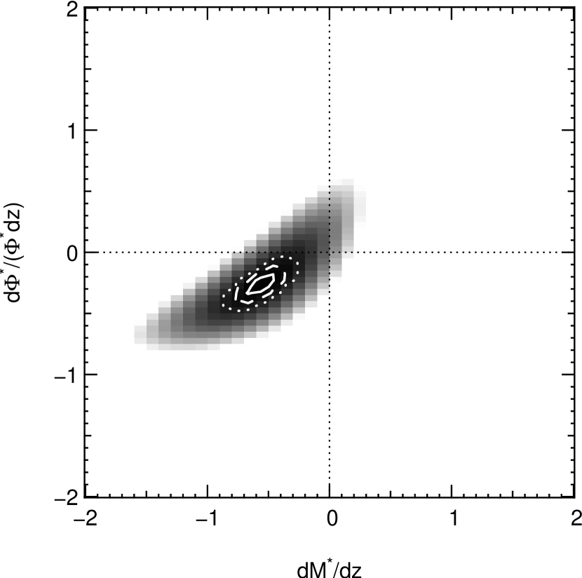
Figure 12: $\chi^{2}$ contours (left panel) and likelihood contours (right panel) for the luminosity function evolution parameters (see text). The contours shown correspond to the $1\sigma$, $2\sigma$, and $3\sigma$ confidence levels.

The results of this approach are shown in the left panel of Fig. 12 and the most likely values of $\mu$ and $\nu$ are listed in Table 2, along with the results from the analysis of the spectroscopic sample in MUNICS V.

6.2 A likelihood-based approach using unbinned data

The luminosity function is very steep at its bright end. When the number of very bright (and therefore rare) galaxies in the sample is small, binning of these data in magnitude must be taken with skepticism. As the distribution of objects within any bin will not be uniform and we are dealing with small numbers of objects, the choice of bin centers and widths might influence the outcome of the analysis. Hence we develop a maximum likelihood based method avoiding having to bin the data to determine the values of the evolution parameters $\mu$ and $\nu$.

Maximum likelihood methods (using binned and unbinned data) have been used in the past by many authors to construct luminosity functions and derive their parameters in various parametric and non-parametric ways (see, e.g., Sandage et al., 1979; Efstathiou et al., 1988; Lin et al., 1996, and references therein). These methods usually suffer from the inconvenience that the normalization has to be determined independently from the shape of the LF. The method presented here allows the shape and normalization (evolution) parameters to be determined simultaneously.

We start with a set of $N_{\mathrm{obs}}$ observed galaxies of absolute magnitudes $M_{i}$ and redshifts $z_{i}$. Assuming a luminosity function, $\Phi_{\mu\nu}(M,z)$, and parameterizing its redshift evolution as described before (Eqs. 5 and 6), one can write the probability of observing galaxy $i$ having the properties $M_{i}$ and $z_{i}$ as

$$P(M_{i},z_{i}|\Phi_{\mu\nu})\,dM\,dz\;=\;\frac{\Phi_{\mu\nu}(M_{i},z_{i})(dV(z_{i})/dz)}{N_{\mathrm{model}}}\,dM\,dz.$$ (9)

The normalization, $N_{\mathrm{model}}$, is the double integral over magnitude and redshift of the LF, and hence equal the total number of galaxies expected in the sample if the LF evolves according to our parametrization:

$$N_{\mathrm{model}}\;=\;\int_{z_{\mathrm{min}}}^{z_{\mathrm{max}}}\,\int_{M_{\mathrm{min}}(z)}^{M_{\mathrm{max}}}\Phi_{\mu\nu}(M,z)\,\frac{dV}{dz}\,dM\,dz$$ (10)

Here we need to take the redshift and magnitude limits of the survey into account. The galaxies are taken to be in the redshift range $z_{\mathrm{min}}\ <z<z_{\mathrm{max}}$, and to have absolute magnitudes $M_{\mathrm{max}}<M<M_{\mathrm{min}}(z)$.

The lower magnitude limit is clearly a function of $z$, and can be written as

$$M_{\mathrm{min}}(z)\;=\;m_{\mathrm{min}}-2.5\,\log(1+z)-k_{c}(z)-D_{m}(z),$$ (11)

where $m_{\mathrm{min}}$ is the completeness limit of the survey in apparent magnitude, $k_{c}(z)$ is the (type-dependent) $k$-correction at redshift $z$, and $D_{m}(z)$ is the distance modulus. The $k$-corrections for each object are obtained from its best-fitting SED (see Sect. 3).

Since we do not want to deal with incompleteness corrections here, we set

$$m_{\mathrm{min}} = 18.7\quad\mathrm{in~{}the}~{}K~{}\mathrm{band}$$

$$z_{\mathrm{min}} = 0.4$$

$$z_{\mathrm{max}} = 1.0$$

where MUNICS is to be considered complete (see MUNICS IV for the detailed completeness analysis).

Note that Eq. 9 cannot be used to determine the normalization, $\Phi^{*}$, or its evolution with redshift, $\mu$, since the dependence on $\Phi^{*}$ cancels out (see also the method presented in Lin et al., 1996). A handle on the normalization can be obtained by observing that the total number of objects in the sample, $N_{\mathrm{obs}}$, must be reproduced by any successful model, $\Phi_{\mu\nu}$, leading to a boundary condition for Eq. 9. The total number of objects in the sample is by itself subject to uncertainty, obeying at least Poisson statistics (assuming that the total survey volume is large enough such that fluctuations due to large scale structure are averaged out). Instead of a boundary condition, we thus add a second term to Eq. 9 taking the Poisson noise in $N_{\mathrm{obs}}$ into account to obtain the final likelihood function

$$\ln\mathcal{L}\;=\;\mathop{\sum}_{i=1}^{N_{\mathrm{obs}}}\ln P(M_{i},z_{i}|\Phi_{\mu\nu})-\frac{1}{2}\left(\frac{N_{\mathrm{model}}-N_{\mathrm{obs}}}{\sqrt{N_{\mathrm{obs}}}}\right)^{2},$$ (12)

The results of this maximum likelihood approach are shown in the right panel of Fig. 12 and the most likely values of $\mu$ and $\nu$ are listed in Table 2. The dashed line in Fig. 10 shows a Schechter function evolved with $z$ using these numbers.

7 Discussion

The $\chi^{2}$ estimates for $\mu$ and $\nu$ yield a mild decrease in number density of 30% to $z=1$ ($\mu=-0.30\pm 0.21$) accompanied by a brightening of the galaxy population by $0.64\pm 0.21$ mag. The uncertainties of the parameters are large, though, because of the relatively large uncertainties of the values of the LF in the individual bins, and because the Schechter LF parameters are almost degenerate if the faint end below $L^{*}$ cannot be measured (at the steep bright end, negative density evolution can be counterbalanced by brightening).

The results from the likelihood estimator are fully consistent with the $\chi^{2}$ estimates, with their uncertainties being much smaller, though (see comparison in Table 2). The likelihood estimator gives 25% number density evolution ($\mu=-0.25\pm 0.05$) and a brightening of $0.53\pm 0.07$ mag. $\mu=0$ is excluded at high confidence ($\sim 4\sigma$). The reason for the much steeper contours of the likelihood surface compared to the $\chi^{2}$ estimator come from the tightness of the constraint in total number of galaxies (Eq. 10). This number is very sensitive to small changes in the Schechter parameters, and therefore provides a very strong constraint on the allowed region in parameter space.

It well worth noting that the parameter estimates obtained by both methods presented here agree with the best estimate obtained in MUNICS V from the spectroscopic sample alone. This makes us confident that the results presented here based on photometric redshifts are, indeed, robust. The formal uncertainties we derive in this work are, however, much smaller than those of the analysis of the purely spectroscopic sample. This is entirely due to the sample size which is a factor of 10 larger than the spectroscopic one in MUNICS V. The results presented here are also consistent with the recent estimate based on a spectroscopic sample by Pozzetti et al. (2003), finding brightening by $0.54\pm 0.12$ magnitudes to $z=1$ and at most a mild decrease ($<30\%$) in number density of red luminous objects.

Obviously, the results of both estimators crucially depend on the parameters assumed for the local ($z=0$) values of the luminosity function. We estimate the impact on the parameters due to this by using a direct fit of a Schechter function to the lowest redshift bin ($0.4<z<0.6$) of the MUNICS sample itself (upper left panel in Fig. 10) as a reference instead of the $z=0$ measurement. The results are effectively unchanged, being consistent within the $1\sigma$ uncertainties in both cases, in fact being almost identical for the $\chi^{2}$ estimator.

Another possible source of systematic error is possible incompleteness in the MUNICS photometric catalogs at high redshift. This would effect the validity of the spectroscopic results in MUNICS V alike since the objects for spectroscopy are selected from the same photometric catalog. The completeness analysis presented in MUNICS IV concluded that detection probabilities are high independent of the sources’ radial profile out to $z\sim 1$, but that photometry suffers from severe biases for bulge-dominated systems where the lost light fraction can be high for the highest luminosity objects. For lower luminosity objects around $L^{*}$ the photometry recovers the total magnitudes well. This is a consequence of the relation between surface brightness and total luminosity for elliptical galaxies. This effect scatters very bright objects towards lower luminosities. Since bright objects are very rare, the effect on the shape of the LF around $L^{*}$ is small, but can be severe at $L\gg L^{*}$. The total magnitude of disk dominated systems are well recovered regardless of total luminosity. Unfortunately, one cannot correct for this effect without assuming a distribution of morphological types or suitable high resolution imaging which is still unavailable for a sample of this size.

To investigate whether our results are sensitive to these effects, we repeat the analysis described above using a number of restricted redshift ranges. Firstly, lowering the upper limit in redshift down to $z=0.8$, we find that the estimate for the density evolution changes by not more than $\Delta\mu=0.08$ with the evolution in luminosity being practically unaffected. The error in $\mu$ increases by $\sim 50\%$, though, because of the smaller number of objects in the restricted-redshift samples. Secondly, we exclude objects at $z<0.6$, since the form of the LF in this bin might be altered at the bright end by the use of photometric redshifts (see Sect. 4.2 and Fig. 9). The result of our analysis did not change significantly, since we use all objects to estimate the value of the evolution parameters rather than relying on determinations in individual redshift bins.

Finally, the faint end slope, $\alpha$, plays a role in our analysis. The current sample does not go deep enough to constrain $\alpha$, which is therefore kept fixed at its local value. The $\chi^{2}$ estimator is not very sensitive to the actual value of $\alpha$, since the faint part of the LF is not sampled much, and the bins are weighted by their $S/N$, such that the total $\chi^{2}$ is dominated by the $L^{*}$ region (where objects are already numerous and $V_{\mathrm{max}}$ corrections are not yet important).

The maximum likelihood estimator is, however, sensitive to the adapted value of $\alpha$. Again, this is because of the tightness of the total-number constraint and the fact that faint objects dominate in number (for all likely values of $\alpha$). We can estimate the size of the systematic error associated with this by using a value of $\alpha=-1$ and repeating the analysis. The model predicts fewer galaxies in this case, and therefore the amount of density evolution required is lower, $\mu=0.15$. On the other hand, the LF in our lowest redshift (still $z=0.5$) bin is inconsistent with $\alpha=1$ (fixing $\Phi^{*}$ to its local value) at the $\sim 2\sigma$ level.

8 Summary

We present a measurement of the evolution of the rest-frame $K$-band luminosity function to $z\sim 1$ using a sample of $K$-selected galaxies drawn from the MUNICS dataset.

Distances and absolute $K$-band magnitudes are derived using photometric redshifts from template SED fits to BVRIJK photometry. These are calibrated using $>500$ spectroscopic redshifts from a spectroscopic follow-up program described in MUNICS V. A method for obtaining templated SEDs matching the properties of the sample is presented and the photometric redshift estimation is explained. We obtain redshift estimates having a rms scatter of $0.055$ and no mean bias.

We use Monte-Carlo simulations to investigate the influence of the errors in distance associated with photometric redshifts on our ability to reconstruct the shape of the LF (Fig. 9).

We construct the rest-frame $K$-band LF in four redshift bins spanning $0.4<z<1.2$ (Fig. 10) and use two different estimators to derive likely values for the evolution of $\Phi^{*}$ and $M^{*}$ with redshift. While the first estimator relies on the value of the luminosity function binned in magnitude and redshift, the second estimator uses the individually measured $\{M,z\}$ pairs alone. Our results are shown in Fig. 12 and are summarized in Table 2. In both cases we obtain a mild decrease in number density by $\sim 25\%$ to $z=1$ accompanied by brightening of the galaxy population by $0.5$ to $0.7$ mag. These results are fully consistent with an analogous analysis using only the spectroscopic MUNICS sample (MUNICS V).

Among the sources of systematic errors are the local values of the parameters of the LF, especially the faint end slope, and possible incompleteness and biases in the photometry (discussed in detail in MUNICS IV) present in the sample. We conclude that these have some influence on our analysis, sometimes affecting the two estimators in different ways, but that these effects do not influence the general conclusion of this work, namely that there is a mild decrease in total number density of $20\%$ to $30\%$ to $z\sim 1$ and brightening by $0.5$ to $0.7$ mag, taking the systematic errors into account.

To interpret these results in terms of a picture of galaxy evolution is not straight-forward. While the change in characteristic luminosity is consistent with models of passive evolution of the stellar populations, we also have to account for the evolution in number density. Since the $K$-band light traces stellar mass, we may attribute a change in $K$ band luminosity function either to a change in the mass-to-light ratio alone (passive evolution) or to a combination of a change in $M/L$ and in stellar mass. A change in stellar mass can be due to star formation and/or due to merging and accretion. These models cannot be discriminated on basis of the luminosity function alone. Note, however, that in MUNICS III we have assumed a model of passive evolution of the mass-to-light ratio to assign stellar masses to the galaxies in the sample. This model assumed a maximum mass at the given $K$-band light by having all stars form at $z=\infty$. Analysis of the number density of objects as a function of stellar mass showed that the total number of galaxies changes only very little (like in this study), but that the number density of systems more massive than $5\times 10^{10}h^{-2}\mathcal{M}_{\odot}$ does decline, and the number density of systems more massive than $1\times 10^{11}h^{-2}\mathcal{M}_{\odot}$ declines even faster, a pattern which is qualitatively consistent with hierarchical clustering, although these models still tend to predict a more rapid decline in number density of massive systems with redshift.

A PLE model for the evolution of $M/L$ for the whole galaxy population is clearly too simplistic and provides only an upper envelope to the stellar mass as a function of redshift. A more proper analysis has to model the mass-to-light ratio of each object individually and take star formation and dust extinction into account. We therefore postpone further interpretation to a later paper (Drory et al. 2003, in preparation; MUNICS VI) where we use the photometry and spectroscopy combined with stellar population models to investigate the evolution of the stellar masses as a function of cosmic epoch.

Field	Area/arcmin2		Field	Area/arcmin2
S2F1	118.7		S5F5	107.6
S2F5	124.1		S6F1	130.8
S3F5	115.3		S6F5	140.2
S5F1	121.9		S7F5	139.1

Table 1: List of the Mosaic Fields with best photometric homogeneity, good seeing, and similar depth. The total area amounts to 997.7 square arcmin (0.28 square degrees). There are $\sim 5000$ objects in the corresponding source catalog

Method	$\mu=\frac{1}{\Phi^{*}(0)}\frac{d\Phi^{*}}{dz}$	$\nu=\frac{dM^{*}}{dz}$
max. likelihood	$-0.25\pm 0.05\,(1\sigma)\;\;0.17\,(3\sigma)$	$-0.53\pm 0.07\,(1\sigma)\;\;0.18\,(3\sigma)$
$\chi^{2}$	$-0.30\pm 0.41\,(1\sigma)\;\;0.59\,(3\sigma)$	$-0.64\pm 0.35\,(1\sigma)\;\;0.51\,(3\sigma)$
Spectroscopy (MUNICS V)	$-0.35\pm 0.5$	$-0.7\pm 0.3$

Table 2: Max. likelihood and $\chi^{2}$ estimates (see text) for the evolution of the Schechter parameters of the rest-frame $K$-band luminosity function to $z=1$. The results obtained by (Feulner et al., 2003; MUNICS V) by analyzing the spectroscopic sample alone are listed for comparison.

Figure 2: Final SED library used to determine photometric redshifts. Note that there are no strongly star forming (young) SEDs in the final set, as can be expected in a $K$-band selected sample. Also noteworthy is the fact that we definitely need dust-reddened SEDs.

Figure 4: Left panel: Comparison of photometric and spectroscopic redshifts for $\sim 500$ objects in five survey patches (different symbols). Right panel: The histogram of the redshift errors. The rms scatter is approximately Gaussian (dotted line: best-fit Gaussian) of a width $\sigma$ = 0.055 and an insignificant mean deviation from the unity relation of $\langle\Delta z\rangle=-0.005$.

Figure 6: Comparison of photometric redshifts from the older VRIJK MUNICS sample used in MUNICS III with the current BVRIJK sample used in this work.

Figure 7: Left panel: the $M_{K}$ – $z$ relationship for the total MUNICS sample of 5132 galaxies using photometric redshifts. Right panel: the photometric redshift distribution of the sample and a best-fit analytic description (dotted line; see text). The distribution of spectroscopic redshifts is also shown for comparison (dashed line).

Figure 8: Cumulative redshift distribution of MUNICS galaxies with apparent $K$-band magnitudes $16<m_{K}<18$. The thin lines are data from individual survey fields, the thick line is the total sample.

Figure 9: Monte-Carlo realizations of the luminosity function to test the susceptibility to random errors in the redshift determination due to the use photometric redshifts. The LFs were simulated with redshift errors $\Delta z$ drawn from a Gaussian of width $0.02$ (upper left), $0.055$ (upper right; this corresponds to the rms redshift error in our sample), $0.1$ (lower left), and $0.2$ (lower right). In each panel, the LF is shown in four redshift bins, $0.4<z<0.6,0.6<z<0.8,0.8<z<1.0,$ and $1.0<z<1.2$ (see text). Each simulation was repeated 10 times, assuming a non-evolving luminosity function of the form the local 2MASS $K$-band LF (dotted line). The simulated LF is generally recovered well, with the known effect that objects are being preferably scattered away from $L^{*}$ becoming apparent at high rms redshift errors.

Figure 10: The final rest-frame $K$-band luminosity function from the MUNICS sample in four redshift bins, $0.4<z<0.6,0.6<z<0.8,0.8<z<1.0,$ and $1.0<z<1.2$. The small filled symbols denote the uncorrected data, the large filled symbols show the final corrected data. Error bars are Poisson errors on the number of objects in each ${M_{K},z}$ bin. The dotted line denotes the local 2MASS $K$-band LF published by Kochanek et al. (2001). The dashed line shows a Schechter function evolved with $z$ using the best-fit values for the evolution parameters $\mu=-0.25$ and $\nu=-0.53$ from Sect. 6. Note that these are not independent fits in each redshift bin but rather a global estimate of the change in $\Phi^{*}$ and $L^{*}$ with redshift (see text).

References

- Bender (2003) Bender, R. 2003, ApJ, submitted
- Bender et al. (2001) Bender, R., et al. 2001, in ESO/ECF/STScI Workshop on Deep Fields, ed. S. Christiani (Berlin: Springer), 327
- Benítez (2000) Benítez, N. 2000, ApJ, 536, 571
- Bromley et al. (1998) Bromley, B. C., Press, W. H., Lin, H., & Kirshner, R. P. 1998, ApJ, 505, 25
- Cimatti et al. (2002) Cimatti, A., et al. 2002, A&A, 381, L68
- Cowie et al. (1996) Cowie, L. L., Songaila, A., Hu, E. M., & Cohen, J. G. 1996, AJ, 112, 839
- Drory et al. (2001a) Drory, N., Bender, R., Snigula, J., Feulner, G., Hopp, U., Maraston, C., Hill, G. J., & de Oliveira, C. M. 2001a, ApJ, 562, L111
- Drory et al. (2001b) Drory, N., Feulner, G., Bender, R., Botzler, C. S., Hopp, U., Maraston, C., Mendes de Oliveira, C., & Snigula, J. 2001b, MNRAS, 325, 550
- Efstathiou et al. (1988) Efstathiou, G., Ellis, R. S., & Peterson, B. A. 1988, MNRAS, 232, 431
- Ellis (1997) Ellis, R. S. 1997, ARA&A, 35, 389
- Feulner et al. (2003) Feulner, G., Bender, R., Drory, N., Hopp, U., Snigula, J., & Hill, G. J. 2003, MNRAS, 342, 506
- Folkes et al. (1999) Folkes, S., et al. 1999, MNRAS, 308, 459
- Gardner et al. (1997) Gardner, J. P., Sharples, R. M., Frenk, C. S., & Carrasco, B. E. 1997, ApJ, 480, L99
- Glazebrook et al. (1995) Glazebrook, K., Peacock, J. A., Miller, L., & Collins, C. A. 1995, MNRAS, 275, 169
- Heidt et al. (2003) Heidt, J., et al. 2003, A&A, 398, 49
- Heyl et al. (1997) Heyl, J., Colless, M., Ellis, R. S., & Broadhurst, T. 1997, MNRAS, 285, 613
- Kinney et al. (1996) Kinney, A. L., Calzetti, D., Bohlin, R. C., McQuade, K., Storchi-Bergmann, T., & Schmitt, H. R. 1996, ApJ, 467, 38
- Kochanek et al. (2001) Kochanek, C. S., et al. 2001, ApJ, 560, 566
- Lilly et al. (1995a) Lilly, S. J., Le Fèvre, O., Crampton, D., Hammer, F., & Tresse, L. 1995a, ApJ, 455, 50
- Lilly et al. (1995b) Lilly, S. J., Tresse, L., Hammer, F., Crampton, D., & Le Fèvre, O. 1995b, ApJ, 455, 108
- Lin et al. (1996) Lin, H., Kirshner, R. P., Shectman, S. A., Landy, S. D., Oemler, A., Tucker, D. L., & Schechter, P. L. 1996, ApJ, 464, 60
- Lin et al. (1997) Lin, H., Yee, H. K. C., Carlberg, R. G., & Ellingson, E. 1997, ApJ, 475, 494
- Lin et al. (1999) Lin, H., Yee, H. K. C., Carlberg, R. G., Morris, S. L., Sawicki, M., Patton, D. R., Wirth, G., & Shepherd, C. W. 1999, ApJ, 518, 533
- Liu et al. (1998) Liu, C. T., Green, R. F., Hall, P. B., & Osmer, P. S. 1998, AJ, 116, 1082
- Madgwick et al. (2002) Madgwick, D. S., et al. 2002, MNRAS, 333, 133
- Maraston (1998) Maraston, C. 1998, MNRAS, 300, 872
- Marzke et al. (1994) Marzke, R. O., Huchra, J. P., & Geller, M. J. 1994, ApJ, 428, 43
- Pozzetti et al. (1996) Pozzetti, L., Bruzual A., G., & Zamorani, G. 1996, MNRAS, 281, 953
- Pozzetti et al. (2003) Pozzetti, L., et al. 2003, A&A, in press
- Ratcliffe et al. (1998) Ratcliffe, A., Shanks, T., Parker, Q. A., & Fong, R. 1998, MNRAS, 293, 197
- Sandage et al. (1979) Sandage, A., Tammann, G. A., & Yahil, A. 1979, ApJ, 232, 352
- Schechter (1976) Schechter, P. 1976, ApJ, 203, 297
- Schmidt (1968) Schmidt, M. 1968, ApJ, 151, 393
- Shapley et al. (2001) Shapley, A. E., Steidel, C. C., Adelberger, K. L., Dickinson, M., Giavalisco, M., & Pettini, M. 2001, ApJ, 562, 95
- Snigula et al. (2002) Snigula, J., Drory, N., Bender, R., Botzler, C. S., Feulner, G., & Hopp, U. 2002, MNRAS, 336, 1329
- Subbarao et al. (1996) Subbarao, M. U., Connolly, A. J., Szalay, A. S., & Koo, D. C. 1996, AJ, 112, 929
- Szokoly et al. (1998) Szokoly, G. P., Subbarao, M. U., Connolly, A. J., & Mobasher, B. 1998, ApJ, 492, 452
- Takeuchi et al. (2000) Takeuchi, T. T., Yoshikawa, K., & Ishii, T. T. 2000, ApJS, 129, 1