Measurement of the Sunyaev-Zel’dovich Increment in massive galaxy clusters

Abstract

We have detected the Sunyaev-Zel’dovich (SZ) increment at $850$$\,\mu$m in two galaxy clusters (Cl$\,0016+16$ and MS$\,1054.4-0321$) using SCUBA (Sub-millimetre Common User Bolometer Array) on the James Clerk Maxwell Telescope. Fits to the isothermal $\beta$ model yield a central Compton $y$ parameter of $(2.2\pm 0.7)\times 10^{-4}$ and a central $850$$\,\mu$m flux of $\Delta I_{0}=2.2\pm 0.7\,$mJy beam^-1 in Cl$\,0016$. This can be combined with decrement measurements to infer $y=(2.38\pm_{0.34}^{0.36})\times 10^{-4}$ and $v_{\mathrm{pec}}=400\pm_{1400}^{1900}\,$km s^-1. In MS$\,1054$ we find a peak $850$$\,\mu$m flux of $\Delta I_{0}=2.0\pm 1.0\,$mJy beam^-1 and $y=(2.0\pm 1.0)\times 10^{-4}$. To be successful such measurements require large chop throws and non-standard data analysis techniques. In particular, the $450$$\,\mu$m data are used to remove atmospheric variations in the $850$$\,\mu$m data. An explicit annular model is fit to the SCUBA difference data in order to extract the radial profile, and separately fit to the model differences to minimize the effect of correlations induced by our scanning strategy. We have demonstrated that with sufficient care, SCUBA can be used to measure the SZ increment in massive, compact galaxy clusters.

1 Introduction

The Sunyaev-Zel’dovich (SZ) effect can be used as a powerful probe of cosmology. Because the intensity of the SZ distortion is virtually independent of redshift, SZ measurements provide an avenue to study clusters and their peculiar velocities to any distance. Additionally, the SZ effect allows independent determination of various cosmological parameters. For example, because the SZ effect’s amplitude is proportional to the electron density along the line of sight through the cluster, $n_{\mathrm{e}}$, while the X-ray amplitude is proportional to $n_{\mathrm{e}}^{2}$, SZ effect data can yield distances to clusters independently from the cosmological distance ladder. This information can then be used to provide estimates of the Hubble constant $H_{0}$ (e.g. Reese et al. 2000).

The physics of the SZ effect is quite simple (Sunyaev & Zel’dovich 1972, Birkinshaw 1999, Carlstrom, Holder & Reese 2002). Cosmic microwave background (CMB) photons can scatter off hot ($T_{\mathrm{e}}\simeq 10^{7}\,$K) electrons in a plasma. A statistical net gain of energy of the photons from the electrons occurs, producing a characteristic distortion in the CMB as seen through the plasma. This distortion produces a decrement in the CMB’s temperature below about 200 GHz, but an increment in the CMB’s temperature above this frequency.

The most important use of SZ increment measurements lies in the determination of the spectral shape of the SZ effect in clusters of galaxies. This shape is the sum of the thermal and kinetic effects together with other sources of emission within the cluster. The kinetic SZ effect is a change in the apparent CMB temperature as seen through the cluster due to the peculiar motion of the cluster relative to the CMB. The kinetic SZ effect may be present in any given cluster and may manifest itself as either a temperature increase or decrease, although it never dominates the thermal effect for expected cluster velocities (Birkinshaw, 1999). Knowledge of the cluster’s properties obtained at several wavelengths can allow separation of these two effects. If the kinetic effect can be isolated, the cluster’s peculiar velocity along the line of sight can be determined. Statistics about large scale flows at a variety of redshifts provide strong constraints on the dynamics of structure formation. In principle, detailed measurement of the SZ spectral shape can also constrain the cluster gas temperature through the relativistic correction (Rephaeli 1995, Birkinshaw 1999, Colafrancesco, Marchegiani, & Palladino 2003).

High frequency measurements can also help separate contaminants such as dusty galaxies which may exist in millimetric measurements, since the dominant sub-mm point sources differ from those seen at longer wavelengths.

Measurement of the Sunyaev-Zel’dovich (SZ) effect increment in galaxy clusters has been an elusive and important goal of observational cosmology for over a decade. While measurements of the SZ effect decrement are common (Birkinshaw 1999, Carlstrom, Holder & Reese 2002), measurement and study of the increment has been less successful. This is largely because current instruments generally lack the sensitivity to measure small amplitude, extended, positive signals in the sky. Also, other positive flux sources in a cluster field can confuse SZ measurements (Loeb & Refregier 1997, Blain 1998). However, experiments working near the null of the thermal SZ effect like SuZIE (Holzapfel et al., 1997), and ACBAR (Peterson et al., 2002) are beginning to yield results. The balloon-borne experiment PRONAOS has had limited success in SZ increment measurements (Lamarre et al., 1998), and other detections are also claimed (e.g. Komatsu et al. 1999). Recently, Benson et al. (2003) have performed this type of measurement in six galaxy clusters, and find that measurement of any given cluster’s peculiar velocity is difficult.

Measurement of the SZ increment is difficult for a variety of reasons, including the amplitude of the atmospheric signal at sub-mm wavelengths. $450$$\,\mu$m and $850$$\,\mu$m observations take advantage of windows in the opacity of the sky at these wavelengths, but successful observation of any astronomical source in the sub-mm regime still requires non-trivial atmospheric subtraction techniques. Additionally, because the SZ effect is a small amplitude signal extended across a relatively large region of the sky, sensitive instruments which can sample a range of spatial frequencies are required. Care must be taken when reconstructing the spatial shape of the SZ effect from data recorded as differences between two or more telescope pointings. As point sources are expected to be a major contaminant in the sub-mm regime, high resolution is also required to adequately understand their effect in a given field. One of the instruments currently most capable of performing observations of the SZ increment is the Sub-millimetre Common User Bolometer Array (SCUBA; Holland et al. 1999). This instrument provides enough sensitivity and angular resolution to detect and remove point sources (including lensed background sources) from the data. SCUBA also samples large enough regions of the sky to constrain the shape of the SZ increment in moderate to high redshift clusters. However, even with these characteristics, measurement of the SZ increment with SCUBA is not trivial.

2 Observations

The bulk of the data discussed here was obtained on November $10$ and $11$, $1999$ at the James Clerk Maxwell Telescope (JCMT) at the summit of Mauna Kea, Hawaii. The JCMT combines a high, dry site with a $15$ metre dish and sensitive instruments. SCUBA, attached on the Nasmyth platform of the JCMT, allows simultaneous observations with $91$ $450$$\,\mu$m–band bolometers and $37$ $850$$\,\mu$m–band bolometers. Because the $450$$\,\mu$m band observes very little SZ increment flux, while the expected peak of the SZ signal occurs near $850$$\,\mu$m, the $450$$\,\mu$m data can act as a monitor of atmospheric emission in this experiment.

SCUBA is sparsely sampled spatially, which is undesirable in this experiment. ‘Jiggling’ to fully sample the array consists of small ($\simeq 6$ arcsec) changes in the position of the beam in a regular pattern. The detectors integrate in each jiggle position for $1.024\,$s. Although $64$ positions are required to fully sample both arrays, this experiment used $16$ positions because it was only necessary to fully sample the $850$$\,\mu$m array. Moreover, executing the jiggle pattern as quickly as possible is more conservative in terms of residual sky fluctuations.

Variations in the signal produced by atmospheric (sky) noise and thermal offsets from the instrument are removed by rapid chopping together with slower telescope nodding (e.g. Archibald et al. 2002). Rapidly chopping the secondary mirror faster than the rate at which the sky is varying removes much of this atmospheric signal. Nodding the telescope’s primary mirror to a second reference position removes slow sky noise gradients and instrument noise. These motions produce a chop pattern such that the two reference beams are each observed half as often as the source beam (Fig. 1). In the standard SCUBA mapping mode, the chop occurs at about $8$ Hz and the nod occurs at about $1/16$ Hz. Although a chop throw in the range $50$ to $100$ arcsec is standard, this experiment requires a chop that does not put significant SZ flux in the reference beams (Fig. 1). For this reason, an extremely large JCMT secondary mirror chop size of $180$ arcsec was used.

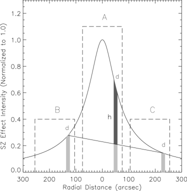
Figure 1: Our chopping strategy in relation to the SZ increment. The solid curve is an isothermal $\beta$ profile (discussed in Section $3.3$) with parameters $\theta_{\mathrm{c}}=50$ arcsec and $\beta=0.75$. The profile’s peak has been normalized such that $\Delta I_{0}=1.0$. The dashed lines show the SCUBA array size at the ‘source’ position marked ‘A’, and the two reference positions, ‘B’ and ‘C’. The filled areas marked ‘d’ show the FWHM of one bolometer, and indicate the bolometer’s position over an observation. SCUBA jiggle mapping gives data in the form $h=d_{\mathrm{A}}-(d_{\mathrm{B}}+d_{\mathrm{C}})/2$ for each bolometer. Because it is sensitive only to differences in SZ flux between the source and two reference beams, $h$ contains much of the information about the SZ effect amplitude, although this is the same information contained in the shape within the array size. However, the JCMT does not have high enough resolution to rely on the differenced SZ shape alone. Using the $850\,$$\,\mu$m array average (that is, the mean of every bolometer’s $h$) to remove the atmospheric emission at each time step subtracts a flux about the same size as $h$, which destroys the information about the SZ effect amplitude in this data.

$89\,$ks of data were taken, split between several fields. The CSO $225\,$GHz $\tau$-meter was not operational for either observing shift, so we relied on skydips to measure the atmospheric optical depth, $\tau_{850}$, in our data set. Both nights had relatively constant $\tau_{850}$, but the first evening had a lower average ($\tau_{850}\simeq 0.15$) than the second ($\tau_{850}\simeq 0.3$). Uranus was used as a calibration source throughout.

Three clusters and three blank fields were observed during this run (see Table 1 for details), referred to as Cl$\,0016$, MS$\,0451$, MS$\,1054$, Blank $02$, Blank $09$ and Blank $25$ hereafter. $23\,$ks of additional data were collected with an aluminum reflector masking the aperture of SCUBA. These data are used as null tests to study SCUBA’s behaviour under both optical and electrical influences (blank sky data) and electrical influences only (reflector data).

Additional data were taken at the JCMT on October $2$, $3$, and $6$, $2002$ in the same manner as the $1999$ run. Both Cl$\,0016$ and another blank field, Blank $21$, were mapped. In addition to the jiggle mapping, photometry of possible point sources in the Cl$\,0016$ field were performed. The photometry used a $9$ point jiggle pattern with $1$ arcsec spacing and a $60$ arcsec chop throw. Bolometer G9 of the SCUBA array was not operating properly during this run and its data are not used here. A total of $13\,$ks of data were taken in 2002; how they are combined with the earlier data is discussed below.

3 General Analysis

3.1 Data Preparation

The data are deswitched, flat-fielded and corrected for atmospheric extinction with surf (the SCUBA User Reduction Facility, Jenness & Lightfoot 1998). Extinction correction is performed by calculating the airmass at which each bolometer measurement was made, and then multiplying by the zenith sky extinction at the time of the measurement to give the extinction optical depth along the line of sight. Each data point is then multiplied by the exponential of the optical depth to give the value that would have been measured in the absence of the atmosphere. The photometric calibration of deep SCUBA fields like those presented here is known to be accurate to about 15 per cent (Borys 2002, Archibald et al. 2002), although $\sim 2/3$ of this uncertainty is due to error in the absolute calibration of the planets’ flux.

It is well documented that the deswitched $450$$\,\mu$m and $850$$\,\mu$m time streams are highly correlated, and that this correlation stems primarily from atmospheric noise (e.g. Jenness, Lightfoot, & Holland 1998, Borys et al. 1999, Archibald et al. 2002). The standard method of removing atmospheric noise from an array is to subtract the array average from each bolometer at each time step. However, most of the information about the SZ flux in this measurement is contained in the difference between the source and reference beam fluxes (see Fig. $1$) rather than in the shape of the SZ emission across the field of view. Therefore, removing the $850\,$$\,\mu$m array average at each time step would drastically reduce the inferred SZ emission. However, because the SZ effect is small at $450\,$$\,\mu$m, using that band’s data should mitigate this problem. A least-squares linear fit of the $450$$\,\mu$m array average to the $850$$\,\mu$m array average at each time step is used to obtain a linear coefficient $C_{1}$ and an offset $C_{0}$ (hereafter referred to as the $\left\langle 450\,\mu\mathrm{m}\right\rangle$ method). These fit parameters and the $450$$\,\mu$m array averages are then used in place of the $850$$\,\mu$m array average to subtract the atmospheric noise at each time:

$$S_{b}^{850}(t)=R_{b}^{850}(t)-\left(C_{1}\left\langle R^{450}(t)\right\rangle+C_{0}\right),$$ (1)

where $S_{b}^{850}(t)$ is the corrected data at time step $t$ for bolometer $b$, $R_{b}^{850}(t)$ is the raw, double-differenced and extinction corrected data at time step $t$ for bolometer $b$, the angled brackets denote an average over the whole array, and the superscripts denote wavelength. The fits are performed separately for each (approximately $20$ minute) observation. $C_{1}$ removes the atmospheric emission on scales of about $1\,$s, while $C_{0}$ removes the atmospheric average over periods long compared to the telescope nod time. The value of $C_{1}$ and $C_{0}$ do not vary by more than 10 per cent over an observation; this is consistent with the results of Borys et al. (1999). $C_{1}$ is typically $0.6$ and $C_{0}$ is of order $1\,\mu$V in our data set. The linear Pearson correlation coefficients of the $450$$\,\mu$m and the $850$$\,\mu$m time streams are on average $0.95$ and never less than $0.90$ for these observations. The average ratio of the variance of $S_{b}^{850}$ in the time stream of the $\left\langle 450\,\mu\mathrm{m}\right\rangle$ atmospheric subtraction method to the variance of the $850\,$$\,\mu$m time stream in the standard surf atmospheric subtraction method is $1.15$. This implies that the $\left\langle 450\,\mu\mathrm{m}\right\rangle$ method is slightly inferior for removing atmospheric noise. However, this approach is required for the analysis of SZ data, since it allows retention of information on angular scales up to that of the chop throw.

Table 1: Experimental target field parameters, including field names and coordinates, on source integration times, and dates of observation.

Target	Field Type	RA (2000)	DEC (2000)	Integration	Observation
				Time (ks)	Dates
Blank $02$	Blank Field	2:22:59.9	+4:59:57	$2.5$	11 Nov. 1999
Blank $09$	Blank Field	9:00:00.0	+10:02:00	$9.4$	10,11 Nov. 1999
Blank $21$	Blank Field	21:30:00.0	+16:30:00	$7.2$	03,06 Oct. 2002
Blank $22$	Blank Field	22:17:25.1	+0:12:59	$8.8$	11 Nov. 1999
Cl$\,0016$+$16$	Cluster Field	0:18:33.7	+16:26:04	$12.2$	11 Nov. 1999, 02,03 Oct. 2002
MS$\,0451$-$03$	Cluster Field	4:54:11.5	$-3$:00:52	$15.1$	10,11 Nov. 1999
MS$\,1054$-$03$	Cluster Field	10:56:57.4	$-3$:37:24	$15.1$	10,11 Nov. 1999

Of the seven target fields, three are unusable for this experiment in some way. A fundamental requirement of this analysis method is high enough signal to noise ratio that it is possible to determine the location of point sources in a field and remove them. However, the Blank $02$ field had only a short integration time (see Table 1), hence it is not included in the results of this experiment. Blank $22$ was a poor choice for a control field, because it contains large point sources which corrupt it for our purposes; Chapman et al. (2001) examine this field in detail. The MS$\,0451$ field contains a sub-mm bright gravitationally lensed arc serendipitously discovered when combining this data with previous observations (Chapman et al., 2002). Although an interesting target in its own right, the $\simeq 12\,$mJy beam^-1 resolved arc dominates the sub-mm emission in this cluster (Borys et al., 2003), making measurement of the SZ increment impossible with these data.

3.2 Point Source Removal

Recognition and removal of point sources, especially unbiased handling of lensed background sources, is important in this experiment (Loeb & Refregier 1997, Blain 1998). We adopt the following procedure. The measured flux differences are binned according to the spatial position of the ‘source’ beam. The standard method of presenting a SCUBA image is to convolve the binned data set with the telescope point spread function (PSF). Maps made by this method are shown in Fig. $2$ in order to indicate the locations of possible point sources and to exhibit their consistency with the same fields in Chapman et al. (2002). However, these images are not used as part of the quantitative analysis.

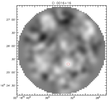
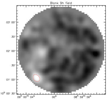
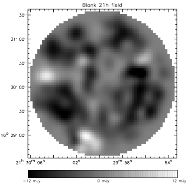
Figure 2: Maps of our target fields using a standard map-making procedure (similar to the surf map-making algorithm). These maps are not used at any point in our analysis, except to serve as a check that large point sources are not present in the data. Contours show the point source cutoff levels in each field (quoted in the text). The 1$\sigma$ rms values of these maps are: 2.9 mJy in Cl$\,0016$; 3.3 mJy in MS$\,1054$; 3.6 mJy in Blank $09$; and 3.9 mJy in Blank $21$. The fluxes and (possible) locations of point sources found and removed from later analysis are given in Table $2$.

Instead, the binned flux differences are convolved with a wavelet similar to a ‘Mexican Hat’ function:

$$\psi(\theta)=\psi_{0}\;\left(1-\frac{\theta^{2}}{2\sigma_{\mathrm{w}}^{2}}\right)\exp\left(\frac{-\theta^{2}}{2\sigma_{\mathrm{w}}^{2}}\right).$$ (2)

Here $\theta$ is an angular distance and $\sigma_{\mathrm{w}}$ is a parameter charactering the wavelet’s width. The normalization $\psi_{0}$ is set such that the flux from a point source placed in a blank field is returned identically at $\theta=0$. This wavelet is more useful than the telescope PSF in this analysis because it returns an amplitude which is insensitive to the average value in the map, which is not expected to be zero in an SZ experiment. The wavelet’s width was chosen to be $\sigma_{\mathrm{w}}=6.3$ arcsec, slightly smaller than the $\sigma$ corresponding to the FWHM of the telescope, because this value maximizes the signal to noise ratio in simulated measurements. After convolution with this function, the positive and negative extrema in the maps are the locations of possible point sources in the source and reference beams respectively (Table 2).

Table 2: Candidate point sources which are removed.

Field	Flux (mJy)	RA (2000)	DEC (2000)
Cl$\,0016$	$10$	0:18:32.7	+16:25:18
MS$\,1054$	$-11$	10:56:52.5	-3:37:27
MS$\,1054$	$-12$	10:56:53.0	-3:37:45
Blank $09$	$13$	9:00:02.4	+10:01:02

The philosophy of this experiment’s point source removal scheme is not to develop a list of point sources per se, but rather to remove the flux contributed by any point-like source. In the simple method utilized here, possible point sources in a field are removed by adopting a single flux level above which sources are found. The limiting flux level is estimated based on atmospheric extinction, integration time and the noise equivalent flux density. For each field, we use the following thresholds: 9 mJy in Cl$\;0016$, 9 mJy in MS$\,1054$; 11.5 mJy in Blank $09$; and 13 mJy in Blank $21$. It is found that the point source list matches that found in Chapman et al. (2002) well. The estimated variance given by this method and the actual mean variance of the pixels agree to 10 per cent or better in each field.

By determining the reference beam positions at which most of the negative flux originates, it is found that the ‘two’ negative point sources in MS$\,1054$ are, in fact, probably caused by one bright source. The source appears to be two sources because the MS$\,1054$ field was observed only at the beginning and the end of the Nov. 11 1999 shift. The field rotated during the interval, thereby extending the single source into ‘two’ apparent sources. Our best estimate of this source’s true position is 10:57:03.5 $\pm 2.0$ seconds in right ascension and $-3$:39:00 $\pm 60$ arc seconds in declination. Chapman et al. (2002) find another source of similar amplitude in this cluster which did not happen to fall in any of our beams. The presence of these sources is consistent with the source count models (e.g. Smail et al. 2002).

The effect of greater than 3$\sigma$ positive sources is removed directly from the time series using the measured amplitude, the telescope pointing history and the telescope’s PSF. A negative 3$\sigma$ source is equally likely to be in either of the two reference beam positions, so the same approach is not available. Hence, data associated with detected negative sources are simply excised from further analysis.

Monte Carlo simulations have been performed to develop an understanding of the effects of point sources on this data. These simulations are fully explained in Zemcov, Newbury & Halpern (2003) (hereafter ZNH ), and the application of the results found there are discussed in Sections $3.3$ and $5$.

3.3 Model Fitting

Because the SZ effect is extended on the sky, the simplest way to isolate it in a cluster is to fit the data to a model. Since the signal to noise ratio in any given pixel is poor for this data set, a simple isothermal $\beta$ model is adequate:

$$\Delta I^{\mathrm{D}}(\theta)=\Delta I_{0}^{\mathrm{D}}\;\left(1+\frac{\theta^{2}}{\theta_{0}^{2}}\right)^{(1-3\beta)/2}.$$ (3)

Here, $\Delta I_{0}^{\mathrm{D}}$ is a measure of the magnitude of the increment at the centre of the cluster, $\theta$ is the angular distance from the centre, and $\theta_{0}$ and $\beta$ are parameters characterizing the cluster. These parameters have already been determined for these clusters from combinations of X-ray and SZ decrement data (see Table $3$). Although there is some uncertainty in the values of $\beta$ and $\theta_{0}$, the error this causes in the inferred $\Delta I_{0}^{\mathrm{D}}$ is negligible at this experiment’s level of precision. We thus fix the angular dependence and focus on determining the amplitude alone with our SCUBA data.

Table 3: Isothermal $\beta$ profile fit parameters.

Cluster	$\theta_{0}$	$\beta$	$z$	Reference
Cl$\,0016$	$42.3$′′	$0.749$	$0.55$	Reese et al. (2000)
MS$\,1054^{\mathrm{a}}$	$66.0$′′	$0.75$	$0.83$	Jeltema et al. (2001)
Blank $09$, $21$	$50.0$′′	$0.75$		Generic Values
aJeltema et al. (2001) discuss the difficulty of applying an
isothermal $\beta$ profile to MS$\,1054$, which is a double–cored
X-ray cluster.

Because the SZ increment is non-zero at $450$$\,\mu$m and the $450$$\,\mu$m array average is used to remove residual sky noise, the superscript ‘D’ is used as a reminder that the value quoted is actually a difference between the $850$$\,\mu$m signal and the $450$$\,\mu$m array average. Retrieving the $850$$\,\mu$m signal (denoted $\Delta I_{0}^{850}$) from $\Delta I_{0}^{\mathrm{D}}$ will be discussed further below.

Directly fitting the data to an isothermal $\beta$ model differenced according to the telescope pointing history is the most straightforward way to determine the peak SZ increment flux in a given field. Both the $\Delta I_{0}^{\mathrm{D}}$ and the 1$\sigma$ error in $\Delta I_{0}^{\mathrm{D}}$ found from fitting to the differenced isothermal $\beta$ model are listed in Table $4$. The error in $\Delta I_{0}^{\mathrm{D}}$ is found via the correlation matrix of the linear fit. $\sigma(\Delta I_{0}^{\mathrm{D}})$ is the square root of the second diagonal element of this correlation matrix. The fit correlation matrix has very small off diagonal elements, meaning that the fit is not correlated with the (meaningless) voltage offset value.

To test the hypothesis that much of the information about the SZ intensity is contained in the difference $S_{b}^{850}(t)$, its average is calculated over the array at each time step. The mean of these values should be greater than 0 and be detected with approximately the same or slightly less significance as the detection given by the fit to the isothermal $\beta$ model. It is found that the means of the Cl$\,0016$ and MS$\,1054$ fields are approximately $1.5\sigma$ and $2\sigma$ above zero, respectively. We conclude that merely using the shape of the SZ distortion across the SCUBA field of view underestimates its true amplitude.

Note that intensities, $\Delta I_{\mathrm{SZE}}$, are generally quoted in mJy per JCMT beamsize, which is related to temperature change via the derivative of the blackbody distribution:

$$\Delta I_{\mathrm{SZE}}=2\,k_{\mathrm{B}}^{3}\,\Omega\left(\frac{T_{\mathrm{CMB}}}{hc}\right)^{2}\frac{x^{4}e^{x}}{(e^{x}-1)^{2}}\Delta T_{\mathrm{SZE}}$$ (4)

where $x=h\nu/kT_{\mathrm{CMB}}$ is the dimensionless frequency, $T_{\mathrm{CMB}}=2.725\,$K, $\Delta T_{\mathrm{SZE}}$ is the change in CMB temperature due to the SZ effect, and $\Omega=5.74\times 10^{-9}$ steradians per beamsize.

Table 4: SZ model fit results.

Target	$\Delta I_{0}^{\mathrm{D}}$ (mJy beam-1)	$\sigma(\Delta I_{0}^{\mathrm{D}})$ (mJy beam-1)
Cl$\,0016$	$1.5$	$0.5$
MS$\,1054$	$1.5$	$0.7$
Blank $09$	$-0.4$	$0.7$
Blank $21$	$1.1$	$1.0$

It is also desirable to make a crude ‘map’ to check the radial profile of the data. A matrix inversion technique utilizes all of the available data to make a map, including information about the off-source pointings (e.g. Tegmark & Bunn 1995, Wright, Hinshaw & Bennett 1996, Stompor et al 2002, Hinshaw et al. 2003). This method involves dividing the sky into a vector of pixels, creating matrices based on pointing and flux data, and the inversion of a single matrix to create a map. The matrix inversion itself is performed using a Singular Value Decomposition (e.g. Press et al. 1992).

Here, the pixel model of the sky is chosen to be the brightnesses of annular rings centred on the cluster, as this conforms to the approximately circular symmetry expected in the SZ signal. The rings have $40$ arcsec widths to track the radial variation with reasonable signal to noise ratio. Once the fluxes of the annuli including their errors and correlations have been estimated, they can be fit to the isothermal $\beta$ model. The fit is performed using both data and model with a weighted mean of 0. This ensures that the model’s DC term does not falsely increase the measured increment. A generalized $\chi^{2}$ statistic is determined, where $\mathbf{x}_{\mathrm{m}}$ is a pixel’s isothermal $\beta$ model value, and $\mathbf{x}_{\mathrm{d}}$ is a pixel’s data value.

$$\chi^{2}=(\mathbf{x}_{\mathrm{m}}-\mathbf{x}_{\mathrm{d}})_{i}\ \mathbf{C}_{ij}^{-1}\ (\mathbf{x}_{\mathrm{m}}-\mathbf{x}_{\mathrm{d}})_{j}.$$ (5)

Our observational strategy produces non-negligible correlations between the annular pixels which are given in $\mathbf{C}_{ij}$, the pixel–pixel covariance matrix. Explicitly, $\mathbf{C}_{ij}=\left(\mathbf{P}^{\mathrm{T}}\mathbf{N}^{-1}\mathbf{P}\right)^{-1}$, where $\mathbf{P}$ is our pointing matrix and the noise is $\mathbf{N}$. $\mathbf{N}$ is assumed to be diagonal because removing the fit to the $450\,$$\,\mu$m array average effectively acts as a pre-whitening filter. These correlations need to be carefully included when the SZ amplitude is determined using this annular pixel model and an isothermal $\beta$ profile. Fig. $3$ shows the annular pixel fluxes as well as the best fit profile (Equation ($3$)) using the parameters listed in Tables $3$ and $4$. The two methods yield very similar results, although we find that the direct fitting method is more sensitive.

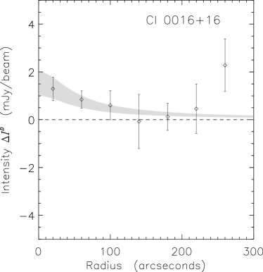
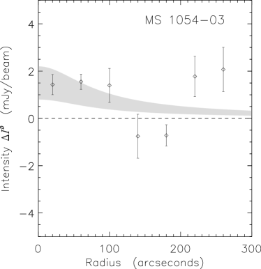
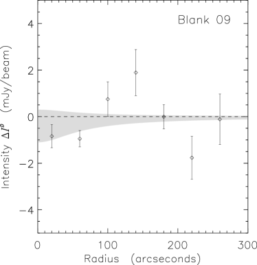
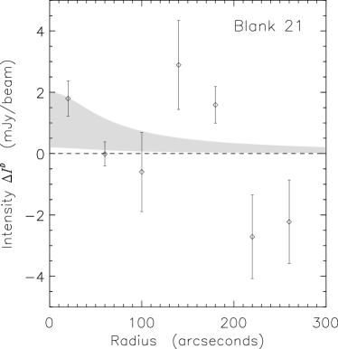
Figure 3: Data points determined via matrix inversion, together with best fit isothermal $\beta$ profiles found from a direct fit for the $4$ target fields shown as $\pm 1\sigma$ confidence regions by the grey band. Note that the isothermal $\beta$ profiles are not best fits to the data points shown but rather use the model in Table $3$ fit directly to the SCUBA differences. The annular points are used to assess the fields’ radial behaviour and to determine the effect of point sources in the beams. As matrix inversion yields data with a mean of zero, the mean of the best fit model is added to the data in these plots. The zero level is shown as a dashed line.

Generally, the figure of merit for the goodness of fit is that $\chi^{2}$ should be approximately the number of degrees of freedom in the data. However, source confusion may have an effect on the applicability of this figure of merit. To test how well $\chi^{2}$ estimates the goodness of fit, Monte Carlo simulations similar to those presented in ZNH are performed in order to determine the probability that the cluster field fits are consistent with the absence of an SZ increment. The direct fit to the isothermal $\beta$ model differences method is used to find $\Delta I_{0}^{\mathrm{D}}$ in simulations containing realistic point sources and with noise levels set to be the same as those in this experiment, but with no SZ increment in the fields. Point sources are removed at the same level as in this experiment; Fig. $4$ shows the results of 200 such simulations. It is found that the fits associated with the highest $10$ per cent of the $\chi^{2}$ statistics always yield drastically incorrect increment values because of point source contamination. We therefore exclude the worst $10$ per cent of the fits. Fig. $4$ also shows the SCUBA results for both clusters, each of which pass the $\chi^{2}$ cutoff. The results overlap, as the fits for these fields give almost the same increment value. If the SZ increment were absent from Cl$\,0016$ and MS$\,1054$, the probability of obtaining the $\Delta I_{0}^{\mathrm{D}}$ found is less than approximately $0.01$ for either cluster.

Figure 4: Results of simulations to determine the effect of confusion on these measurements. This plot shows the cumulative probability of finding an increment value $\Delta I_{0}$ if no increment were present, $P(\Delta I\!>\!\Delta I_{0})$, as a function of fit amplitude $\Delta I_{0}$ found from fitting to the differenced isothermal $\beta$ model. The simulations use realistic noise including point sources and no SZ effect. Point source removal has been implemented (see Section $3.2$ for details). The values determined for the two clusters in this study are shown by the dashed vertical line. This function is not symmetric about zero because gravitational lensing preferentially brightens positive point sources, thereby biasing the point source removal scheme.

The $\chi^{2}$ values found for Cl$\,0016$ are $3.7$ for $6$ degrees of freedom via the seven pixel fit method, and a $\chi^{2}$ of $178402$ for $178406$ degrees of freedom using the direct fit to model differences. We conclude that the fits are fully consistent with the presence of an increment in this cluster.

Our confidence in the parameters found for MS$\,1054$ is less than that for Cl$\,0016$. Based on its $\chi^{2}$ of $13.4$ for $6$ degrees of freedom from fitting the annular pixels to an isothermal $\beta$ model, this cluster would normally be flagged as a poor fit. The fit may be poor because the isothermal $\beta$ model does not describe the distribution of MS$\,1054$’s intracluster electron gas particularly well (Jeltema et al., 2001). However, the fit may become tolerable if the nature of the double–cored electron gas distribution is taken into account. Nevertheless, the reduced $\chi^{2}$ from fitting to the isothermal $\beta$ model differences is $258438$ for $258204$ degrees of freedom in this cluster. The reduced $\chi^{2}$ statistic associated with this fit falls well below the worst 10 per cent of reduced $\chi^{2}$ statistics in the Monte Carlo simulations discussed above. The fit is therefore acceptable based on this criterion.

The parameters determined for the blank fields are also given in Table $4$. From the fits to annular pixels, the Blank $09$ field has a $\chi^{2}$ of $11.7$ for $6$ degrees of freedom and the Blank $21$ field has a $\chi^{2}$ of $13.6$ for $6$ degrees of freedom. The $\chi^{2}$ from fitting to the model differences are poor in both fields. Both fields also seem to exhibit unremoved, confused point sources. The simulations of ZNH show that fields with no SZ increment form a well-defined locus on the $I_{0}$–$\chi^{2}$ plane, and both of the blank fields in this experiment would be inside the confused regime and hence be rejected as SZ increment candidates based on their $\chi^{2}$.

For the purposes of comparison, the line $\Delta I_{0}=0\,$mJy beam^-1 is fit to the data using the direct fit method. The $\Delta\chi^{2}(=\chi^{2}-\chi^{2}_{\mathrm{min}})$ values for these fits are 6.7 for Cl$\,0016$, 6.6 for MS$\,1054$, 0.5 for Blank $09$ and 2.0 for Blank $21$. These values are in good agreement with the significance of the detections.

Although the MS$\,0451$ and Blank $22$ fields were found to be unsatisfactory for this experiment earlier in our analysis, this analysis pipeline also rejects these fields. Both fields have $\Delta I_{0}$ consistent with $0\,$mJy per beam, and poor $\chi^{2}$ due to the number and location of sources within them. This is an objective check that retrieving an SZ increment from data heavily polluted by point sources is difficult.

4 Individual Cluster Analysis & Results

In this section our data are used to determine the $850$$\,\mu$m SZ increment values in Cl$\,0016$ and MS$\,1054$. A maximum likelihood method is used to determine the best fit Compton $y$ parameter (which parametrizes the integrated pressure in the cluster along the line of sight) and, in Cl$\,0016$, the peculiar velocity of the cluster along the line of sight.

4.1 Cl$\,\mathbf{0016}$+$\mathbf{16}$ $\mathbf{\Delta I_{0}^{850}}$ Determination

Worrall & Birkinshaw (2003) find that Cl$\,0016$ has $T_{\mathrm{e}}\simeq 9\,$keV, implying that it has a relativistic electron population which may give a significant correction near the positive peak of the SZ spectrum. Therefore, the corrections found by Itoh, Kohyama & Nozawa (1998), which are good to fifth order in $k_{\mathrm{B}}T_{\mathrm{e}}/m_{\mathrm{e}}c^{2}$, are used to determine the correct shape of the thermal SZ distortion. These corrections, which represent a $10$–$20$ per cent change to the flux at $850$$\,\mu$m for standard cluster parameters, are applied to all of the spectral calculations, and are implicit in the use of the term ‘thermal’ SZ effect below.

Because the SCUBA filters have a finite bandwidth, we need to determine the effective central frequencies of this measurement. This calculation must be performed because the SZ spectrum differs from the grey-body spectra SCUBA usually observes. To do this, the ‘equivalent frequency’ is defined as:

$$\bar{\nu}=\frac{\int_{0}^{\infty}\nu F(\nu)S(\nu)d\nu}{\int_{0}^{\infty}F(\nu)S(\nu)d\nu},$$ (6)

where $F(\nu)$ is the actual SCUBA filter’s response and $S(\nu)$ is the SZ effect spectrum over the region of interest. The results of this calculation are listed in Table $5$; we conclude that the frequency shift from the nominal values are negligibly small.

Table 5: Equivalent $\nu$, $\lambda$ for SZ spectra.

Filter	$\bar{\nu}$	$c/\bar{\nu}$
$850\,$$\,\mu$m	$347\,$GHz	$865\,$$\,\mu$m
$450\,$$\,\mu$m	$652\,$GHz	$460\,$$\,\mu$m

Foreground dust emission could also contaminate the measurement of the SZ increment in these clusters. ISO data are used to estimate the dust contribution. The telescope pointings are used to sample the $180$$\,\mu$m and $90$$\,\mu$m ISO map of the cluster region in exactly the same way as the SCUBA data. Errors for each measurement are determined from the error map and incorporated into the simulated time stream. These data are then fit to the model differences. The $\chi^{2}$ values imply that the fits are very poor; this is expected because any dust emission in the region (Galactic cirrus, extragalactic point sources, or the cluster itself) is unlikely to be distributed like the isothermal $\beta$ model. However, the dust may still contribute to the SZ signal and so must be removed. The dust contribution is determined by fitting a modified black body of the form:

$$I_{\mathrm{d}}(\nu,T_{\mathrm{d}})=\alpha\frac{\nu^{3+\gamma}}{e^{h\nu/k_{\mathrm{B}}T_{\mathrm{d}}}-1}.$$ (7)

Here, the parameters are the spectral index $\gamma$, dust temperature $T_{\mathrm{d}}$, and normalization $\alpha$, which is determined using both of the ISO data points weighted by their errors. $\gamma$ is taken to be $2.0$ and $T_{\mathrm{d}}$ to be $20\,$K, parameters which are typical for ISO–detected cirrus at these wavelengths (e.g. Lamarre et al. 1998). Using this model, the dust emission at $450$$\,\mu$m is determined to be $I_{\mathrm{d}}(660\,\mathrm{GHz})=0.07\pm 0.04$ mJy beam^-1 for Cl$\,0016$. This value is not very sensitive to variations in the parameters $\gamma$ and $T_{\mathrm{d}}$. The fit is corrected for dust emission by the addition of this value, which is a few per cent correction.

Because our analysis scheme subtracts the $450\,$$\,\mu$m flux, a method of retrieving $\Delta I_{0}^{850}$ from $\Delta I_{0}^{\mathrm{D}}$ is required. The actual quantity subtracted from each $850$$\,\mu$m bolometer’s time stream is the average of the $450$$\,\mu$m array at each time step. This average contains the SZ signal sampled as described in Fig. 1, with $\Delta I_{0}^{450}$ being the peak isothermal $\beta$ model amplitude. The average value of the $450\,$$\,\mu$m array is determined by sampling the model SZ profile in the same way as in this experiment. A map is made based on this data, and the average of this map in the field of view is constructed. It is found that there is a linear relationship between the input SZ amplitude and the average of the differenced map, given by $\Delta I_{\mathrm{Ave}}^{450}=A\Delta I_{0}^{450}$, where $A$ is a linear coefficient and $\Delta I_{\mathrm{Ave}}^{450}$ is the average of the difference map over the field of view. This means that $\Delta I_{0}^{850}$ can be found via:

$$\Delta I_{0}^{850}=\Delta I_{0}^{D}+A\Delta I_{0}^{450},$$ (8)

where $A$ depends only on the shape of the isothermal $\beta$ model. $A=0.72$ in Cl$\,0016$, including the gain difference between the $850$$\,\mu$m and $450$$\,\mu$m arrays.

To determine the best fit Compton $y$ parameter and peculiar velocity $v_{\mathrm{pec}}$, we utilize a likelihood function which searches the $y$ - $v_{\mathrm{pec}}$ parameter space for its maximum. Previous decrement measurements at $15\,$GHz (Grainge et al., 2002), $20\,$GHz (Hughes & Birkinshaw, 1998) and $30\,$GHz (Reese et al., 2000) are used alone to determine a best-fit $y$ value, and also in conjunction with our measurement to help constrain both the thermal and kinetic SZ effects in Cl$\,0016$. Alone, these values yield $y=(2.38\pm 0.12)\times 10^{-4}$ in this cluster, assuming $v_{\mathrm{pec}}=0\,$km s^-1. Our value alone yields $y=(2.2\pm 0.7)\times 10^{-4}$ under the same assumption. This measurement is therefore consistent with earlier results.

We find that the $850\,$$\,\mu$m SZ increment value for Cl$\,0016$ is $\Delta I_{0}^{850}=2.2\pm 0.7$ mJy beam^-1. This corresponds to $0.38\pm 0.12$ MJy sr^-1 or $\Delta T_{\mathrm{CMB}}=1.2\pm 0.4$ mK in thermodynamic temperature units. Fig. $5$ shows the corrected $850$$\,\mu$m data point, along with the radio and ISO results. Also plotted are the best fit thermal SZ effect and dust emission spectra, and the position of the $450$$\,\mu$m band–centre for reference.

Figure 5: Sources of extended emission in the Cl$\,0016$ field. The dashed line shows the corrected thermal SZ effect determined from both our $850$$\,\mu$m point and low frequency decrement measurements. The inset shows the low frequency data. The dot-dash line shows the dust emission determined from ISO measurements (asterisks). The best fit kinetic effect is shown as a dotted line. The sum of the thermal and kinetic effects is shown as a solid line. For reference, the position of $450$$\,\mu$m (dotted vertical line) and zero flux (horizontal solid line) are shown. Our $850$$\,\mu$m point is shown as a diamond, and has been corrected for both the $450$$\,\mu$m subtraction and dust emission.

In addition to constraining $y$, the amplitude of the kinetic SZ effect is also constrained by this likelihood analysis. Using both our measurement and the three decrement measurements, it is found that the marginalized best fit parameters are $y=(2.38\pm_{0.34}^{0.36})\times 10^{-4}$ and $v_{\mathrm{pec}}=400\pm_{1400}^{1900}$ km s^-1 in Cl$\,0016$. Assuming $v_{\mathrm{pec}}=0$, these points yield $y=(2.38\pm 0.11)\times 10^{-4}$. Fig. $5$ also shows the inferred kinetic SZ effect from the $850$$\,\mu$m data. This result is therefore only a weak constraint on the line of sight peculiar velocity.

A kinetic SZ effect in Cl$\,0016$ may be mimicked by a primary fluctuation in the CMB, because the spectral distributions of the two effects are the same. However, the primary CMB anisotropies at the scales of this experiment, $\ell>5000$, are about $1\mu\,$K rms (Hu & Dodelson 2002, Borys et al. 1999). This corresponds to a $\pm 0.005\,$mJy beam^-1 signal, which is negligible at our level of precision.

4.2 MS$\mathbf{\,1054-03}$ $\Delta I_{0}^{850}$ Determination

The value of $y$ for MS$\,1054$ is found by determining the difference $I^{850}-AI^{450}$ for the SZ distortions defined by $1.0\times 10^{-5}\leq y\leq 1.0\times 10^{-3}$, where $A=0.81$ for this cluster. The $y$ values giving differences most closely matching the data and 1$\sigma$ error points are the best fitting $y$ parameter and error bars. This method yields $y=\left(2.0\pm 1.0\right)\times 10^{-4}$ for this cluster, including relativistic corrections. These $y$ values correspond to an increment of $\Delta I_{0}^{850}=2.0\pm 1.0\,$mJy beam^-1, or $\Delta T_{\mathrm{CMB}}=1.0\pm 0.5\,$mK.

Because little other relevant data exist for this cluster, further analysis is not possible. The dust contamination cannot be estimated because there are no ISO data, and the available dust maps (Schlegel, Finkbeiner & Davis, 1998), which are of poor angular resolution, provide little spectral information. However, it appears that the dust contamination is at a similar level to that found in Cl$\,0016$, and hence is probably negligible. Although one published estimate of the thermal decrement magnitude already exists for MS$\,1054$ (Joy et al., 2001), a worthwhile estimate of its kinetic effect cannot be made because no explicit $y$ parameter or $\Delta T_{\mathrm{CMB}}$ is available.

5 Discussion

In principle, measurements of the SZ increment, in combination with lower frequency measurements, can yield a great deal of information. For example, the line of sight peculiar velocity and possibly even the cluster temperature can be determined via measurement of the SZ increment. However, measurement of the SZ increment with SCUBA is difficult. There are three essential components which combined to make this experiment a success.

The first component is a carefully planned observational strategy designed to maximize SCUBA’s sensitivity to an SZ signal. Using a large chop throw to reduce the tendency to subtract SZ signal and chopping in azimuth so that sky rotation reduces the effect of point source contamination are both parts of this. Also, using the $450$$\,\mu$m array average to remove the spurious sky signal, thereby keeping SZ information on scales larger than the array size, maximizes the available signal in the data. Controls such as the blank fields, and to a lesser extent the reflector data, are required to check for systematic effects in both the instrument and analysis methods.

The second necessary component of this experiment is the use of custom-designed software to handle the data analysis, which is particularly important for fitting the differenced data directly to a model.

The third important component of this analysis is the removal of point sources in order to reduce their contaminating effect. Because sub-mm bright, high $z$ background sources are relatively common in cluster fields, observations of the SZ increment could suffer prohibitively from the effects of point sources. The basic principle we employ is that point sources affect only a few pixels and hence can be distinguished from an extended SZ effect. Our data have a confusion limit of approximately $0.8\,$mJy beam^-1 for SZ signals. Integration to SCUBA’s fundamental confusion limit of $\simeq 0.5\,$mJy beam^-1 rms (which would require weeks of integration time) gives an SZ confusion of $\sim 0.5\,$mJy beam^-1. Our simulations show negligible reduction in the confusion limit of these observations when point sources with amplitude less than about 5 mJy are removed (ZNH, ). This limit would require approximately 2 shifts of integration time. Unfortunately, decreasing the confusion limit floor below $0.5$ mJy beam^-1 would require higher angular resolution observations. A corollary to this is that SZ increment detections from other experiments with lower resolution than SCUBA, such as SuZIE and ACBAR, may be confusion dominated if unsupported by higher resolution data.

These measurements confirm the SZ effect in 2 galaxy clusters at an amplitude consistent with the measured decrements. A weak constraint on the kinetic effect in Cl$\,0016$ is found which is consistent with the result in Benson et al. (2003). We quote a marginal 2$\sigma$ SZ increment detection in MS$\,1054$, but cannot do much more with the data at this point.

It is clear that large reductions in the uncertainty of the value for the kinetic effect velocity in Cl$\,0016$ will not be achievable because of source confusion with this type of instrument. This means that SCUBA is not capable of determining the amplitude of the kinetic effect in any specific cluster, given the expected level of SZ–derived peculiar velocities (e.g. Sheth & Diaferio 2001). It is likely that the only way to use SCUBA for constraining peculiar velocities is through a statistical survey of many clusters.

Nevertheless, we have demonstrated that, with sufficient care, it is possible to measure the $850$$\,\mu$m increment at the JCMT. Such SCUBA observations of the SZ effect at $850$$\,\mu$m can be combined with measurements at other frequencies to study individual clusters in more detail. Follow–up observations with high resolution sub-mm instruments are likely to become an important part of forthcoming SZ cluster surveys.

This paper has been produced using the Royal Astronomical Society/Blackwell Science LaTeX style file.

References

- Archibald et al. (2002) Archibald E. N. et al., MNRAS, 336, 1
- Birkinshaw (1999) Birkinshaw M., 1999, PhysRep, 310, 97
- Benson et al. (2003) Benson B. A. et al., 2003, Submitted to ApJ (astro-ph/0303510)
- Blain (1998) Blain A. W., 1998, MNRAS, 297, 502
- Borys et al. (1999) Borys C., Chapman S. C., Scott D., 1999, MNRAS, 308, 527
- Borys et al. (2002) Borys C., Chapman S. C., Halpern M., Scott D., 2002, MNRAS, 330, L63
- Borys (2002) Borys C., 2002, PhD Thesis, Univ. British Columbia
- Borys et al. (2003) Borys C., Chapman S. C., Donahue M., Fahlman G. G., Halpern M., Newbury P., Scott D., 2003, Submitted to MNRAS
- Carlstrom, Holder & Reese (2002) Carlstrom J. E., Holder G. P., Reese E. D., 2002, Annu. Rev. Astron. Astrophys., 40, 643
- Chapman et al. (2001) Chapman S. C., Lewis G. F., Scott D., Richards E., Borys C., Steidel C. C., Adelberger K. L., Shapley A. E., 2001, ApJL, 548, L17
- Chapman et al. (2002) Chapman S. C., Scott D., Borys C., Fahlman G. G., 2002, MNRAS, 330, 92
- Colafrancesco, Marchegiani, & Palladino (2003) Colafrancesco S., Marchegiani P., Palladino E., 2003, A & A, 397, 27
- Grainge et al. (2002) Grainge K., Grainger W. F., Jones M. E., Kneissl R., Pooley G. G., Souanders R., 2002, MNRAS, 329, 890
- Hinshaw et al. (2003) Hinshaw G. et al., 2003, Submitted to ApJ (astro-ph/0302222)
- Holland et al. (1999) Holland W. S. et al., 1999, MNRAS, 303, 659
- Holzapfel et al. (1997) Holzapfel W. L., Ade P. A. R., Church S. E., Mauskopf P. D., Rephaeli Y., Wilbanks T. M., Lange A. E., 1997, ApJ, 481, 35
- Hu & Dodelson (2002) Hu W., Dodelson S., 2002, Annu. Rev. Astron. Astrophys., 40, 171
- Hughes & Birkinshaw (1998) Hughes J. P., Birkinshaw M., 1998, ApJ, 501, 1
- Itoh, Kohyama & Nozawa (1998) Itoh N., Kohyama Y., Nozawa S., 1998, ApJ, 501, 7
- Jeltema et al. (2001) Jeltema T. E., Canizares C. R., Bautz M. W., Malm M. R., Donahue M., Garmire G. P., 2001, ApJ, 562, 124
- Jenness & Lightfoot (1998) Jenness T., Lightfoot J. F., 1998, in Albrecht R., Hook R. N., Bushouse H. A., eds, ASP Conf. Ser. Vol. 145, Astronomical Data Analysis Software and Systems VII. Astron. Soc. Pac., San Francisco, p. 216
- Jenness, Lightfoot, & Holland (1998) Jenness T., Lightfoot J. F., Holland W. S., 1998, Proc. SPIE, 3357, 548
- Joy et al. (2001) Joy M. et al., 2001, ApJL, 551, L1
- Kessler et al. (1996) Kessler M. F. et al., 1996, A&A, 315, L27
- Komatsu et al. (1999) Komatsu E., Kitayama T., Suto Y., Hattori M., Kawabe R., Matsuo H., Schindler S., Yoshikawa K., 1999, ApJL, 516, L1
- Lamarre et al. (1998) Lamarre J. M. et al., 1998, ApJL, 507, L5
- Loeb & Refregier (1997) Loeb A., Refregier A., 1997, ApJL, 476, L59
- Peterson et al. (2002) Peterson J. B. et al., 2002, Bulletin of the American Astronomical Society, 201, #59.07
- Press et al. (1992) Press W. H., Teukolsky S. A., Vetterling W. T., Flannery B. P., 1992, Numerical Recipes in C (2nd Ed.), Cambridge, Cambridge
- Reese et al. (2000) Reese E. D. et al., 2000, ApJ, 533, 38
- Rephaeli (1995) Rephaeli Y., 1995, ApJ, 445, 33
- Schlegel, Finkbeiner & Davis (1998) Schlegel D. J., Finkbeiner D. P., Davis M., 1998, ApJ, 500, 525
- Sheth & Diaferio (2001) Sheth R. K., Diaferio A., 2001, MNRAS, 322, 901
- Smail et al. (2002) Smail I., Ivison R. J., Blain A. W., Kneib J.-P., 2002, MNRAS, 331, 495
- Stompor et al (2002) Stompor R. et al., 2002, Phys. Rev. D, 65, 22003
- Sunyaev & Zel’dovich (1972) Sunyaev R., Zel’dovich Y., 1972, Comments Astrophys. Space Phys., 4, 173
- Tegmark & Bunn (1995) Tegmark M., Bunn E. F., 1995, ApJ, 455, 1
- Wright, Hinshaw & Bennett (1996) Wright E. L., Hinshaw G., Bennett C. L., 1996, ApJL, 458, L53