Escape probability methods versus “exact” transfer for modelling the X-ray spectrum of Active Galactic Nuclei and X-ray binaries

In the era of XMM-Newton and Chandra missions, it is crucial to use codes able to compute correctly the line spectrum of X-ray irradiated thick media (Thomson thickness of the order of unity), in order to build models for the structure and the emission of the central regions of Active Galactic Nuclei (AGN), or of X-ray binaries. In all photoionized codes except in our code Titan, the line intensities are computed with the so-called “escape probability approximation”. In its last version, Titan solves the transfer of a thousand lines and of the continuum with the “Accelerated Lambda Iteration” method, which is one of the most efficient and at the same time the most secure for line transfer. We first review the escape probability formalism and mention various reasons why it should lead to wrong results concerning the line fluxes. Then we check several approximations commonly used instead of line transfer in photoionization codes, by comparing them to the full transfer computation. We find that for conditions typical of the AGN or X-ray binary emission medium, all approximations lead to an overestimation of the emitted X-ray line spectrum, which can reach more than one order of magnitude. We show that it is due mainly to the local treatment of line photons, implying a delicate balance between excitations of X-ray transitions by the very intense underlying diffuse X-ray continuum (which are not taken properly into account in escape probability approximations) and the net rate of excitations by the diffuse line flux. The most affected lines are those in the soft X-ray range. Such processes are much less important in cooler and thinner media (like the Broad Line Region of AGN), as the most intense lines lie in the optical and near ultraviolet range where the diffuse continuum is small. We conclude that it is very important to treat correctly the transfer of the continuum to get the best results for the line spectrum. On the other hand the approximations used for the escape probabilities have a relatively small influence on the computed thermal and ionization structure of the surface layers, but in the deep layers, they lead to an overestimation of the ionization state. As a consequence the computed continuum emitted by the back (non-irradiated) side is not correct, and might be strongly overestimated in the EUV range.

1 Introduction

For about two decades, many computations of the structure and emission of irradiated hot media have been performed, to understand the spectra of Active Galactic Nuclei (AGN) or of X-ray binaries. Based on the observations, all interpretations of AGN postulate that their UV-soft X spectrum is emitted by a dense, warm, and optically thick medium (density higher than 10¹² cm^-3, temperature of 10⁵ to 10⁶ K, Thomson thickness of the order of, or greater than, unity), illuminated by an X-ray continuum. Similar conditions are met in X-ray binary stars. This medium can be identified with the atmosphere of an accretion disc in hydrostatic equilibrium (Ko & Kallman 1994, Nayakshin et al. 2000, Ballantyne et al. 2001, Różańska et al. 2002), or with a system of clouds, either of constant density, or of constant pressure (Collin-Souffrin et al. 1996, Dumont et al. 2002). In early models, the disc itself was assumed to be a slab of constant density (Ross & Fabian 1993, and subsequent works). Whatever it is, this medium is assumed to be heated and photoionized by an X-ray continuum extending up to a few hundreds keV.

Similar conditions hold in the atmospheres of the discs in X-ray binaries: they are also dense and thick, and irradiated by a strong X-ray continuum. Their modelling is performed exactly like those of AGN discs (cf. Ko & Kallman 1994).

Several codes have been developed in order to handle such computations. Three codes are particularly designed for Thomson thick media: Nayakshin’s code (Nayakshin et al. 2000), Ross and Ballantyne’s code (Ross et al. 1978, Ross 1979), and our code, Titan, described in Dumont et al. (2000), hereafter called DAC, updated in Dumont & Collin (2001), in Coupé (2002), and finally in the present paper where a new transfer method for the lines (the Accelerated Lambda Iteration method) has been implemented. Nayakshin’s code was especially developed for the irradiated atmosphere of an accretion disc in hydrostatic equilibrium, and Ross code and Titan have been adapted to this case (cf. Ballantyne et al. 2001, and Różańska et al. 2002). A comparison between these codes was performed in the case of a photoionized slab with a constant density, and the resulting spectra are shown in Pequignot et al. (2001). It is clear that they are all different, as a result of the approximations made in the computations, and in spite of the fact that the parameters of the model were exactly the same. One should also mention Hubeny’s code (Hubeny et al. 2000, 2001), which has produced accurate grids of model spectra for accretion disc atmospheres, but is still not adapted to the X-ray irradiated case.

With the advent of the X-ray missions Chandra and XMM-Newton, high resolution spectra of AGN in the soft X-ray range have been obtained showing features in absorption and/or in emission. There is in particular a strong controversy on the identification of the lines in the spectrum of MCG -6-30-15. Branduardi-Raymont et al. (2001) propose that the spectrum is dominated by very intense lines in emission (for instance OVIII L$\alpha$ with an equivalent width of about 100 eV) emitted by the atmosphere of an irradiated relativistic disc, while for Lee et al. (2001) the spectral features are mainly absorption edges and absorption lines of neutral elements locked in a dusty absorber. It is therefore crucial to get good model spectra in order to check the validity of the first hypothesis, and more generally to be able to model the X-ray line spectrum.

Several well-known and publicly available codes are also frequently used for photoionized media (Cloudy and XSTAR in particular). They are very accurate from the point of view of the atomic data and for the number of ions and discrete levels taken into account. In DAC it was shown that the transfer treatment of the continuum performed in these codes (outward only approximation, or escape probability formalism) precludes them to be used for Thomson thick media. We will show that the same restriction holds for the line transfer.

Titan, Ross-Ballantyne’s and Nayakshin’s codes are non-LTE photoionization codes differing both by the treatment of the atomic data and of the transfer. These points have been discussed in some details in Różańska et al. (2002) and in Dumont et al. (2002), so we will not insist on them here. It is sufficient to recall that, as long as atomic data are considered, Nayakshin’s code, which is based on the code XSTAR, is the best. Titan is intermediate between Nayakshin and Ross-Ballantyne codes, as it includes all ions of the ten most abundant elements, and treats them as interlocked multi-level atoms in the case of all hydrogen-like, helium-like, and lithium-like species and a few other ions.

For the transfer of the continuum, Ross-Ballantyne code uses the Kompaneets diffusion approximation, and Nayakshin the variable Eddington factor transfer method with the addition of a Compton scattering operator, while Titan uses the Accelerated Lambda Iteration (ALI, cf. Hubeny 2001, Dumont & Collin 2001). Titan considers the effect of Compton diffusions only in the energy balance, and has therefore to be coupled with the Monte Carlo code NOAR of DAC to take into account Compton scatterings in the high energy continuum.

For the transfer of the lines, Nayakshin’s and Ross-Ballantyne’s codes use the so-called “escape probability approximation”, like Cloudy and XSTAR. It means that the line intensities, the contribution of the lines to the energy balance, to the ionization equilibrium, and to the radiation pressure, are computed in an approximate way, which might or might not give correct results. In this new version of Titan the line transfer is solved now with the ALI method, unlike to the previous version described in Dumont & Collin (2001) where it was solved with a simple Lambda Iteration method (a full description of the present version of the code will be given elsewhere). This method ensures that even the most optically thick lines are accurately computed. Comptonisation of line photons was also recently added to the code as described in Appendix A.

A strong drawback of Titan is that it is time-consuming, and this prevents it from being easily used like the other codes, for instance to build grids of models. This is not only due to the resolution of the transfer in the lines, which requires to solve the transfer for fifteen frequencies inside each line, for several hundreds of lines (presently more than 800, whose majority is optically thick) to be sure to have a good representation of the spectrum and of the structure of the medium, but it is also due to the accurate treatment of the continuum itself, which is necessary as we will see later. Thus one could ask legitimely if it is worth performing these enormous computations, at the expense of other ones (for instance calculating the equilibrium of a very large number of levels like in Cloudy or XSTAR). Note however that the computation time with the ALI method is reduced with respect to the previous transfer method, especially using a diagonal i.e., local approximate operator as we did.

We will not discuss here the impact of the treatment of the continuum, as it was already done in DAC, and we will focus only on the influence of the escape probability approximation when it is used instead of line transfer. We will thus compare different line escape probability approximations with the full transfer treatment, keeping exactly the same method for the transfer of the continuum. It means that we will not be able to compare directly our computations with the Ross-Ballantyne and Nayakshin ones, since they do not use the same method for the transfer of the continuum. But doing that, we can disentangle the influence of the line approximations from that of the treatment of the continuum, which is more important than the lines in defining the temperature and ionization structure.

In this paper we restrict our study to two representative models. We will perform in a forthcoming paper the same comparison for different physical conditions, in order to set limits to the validity of the escape approximations.

In the next section, we summarize the basics of radiation transfer and of the escape probability formalism. Some approximations used in different codes for the escape probabilities are recalled in Section 3. In Section 4 the structure and the emission spectrum of an illuminated slab of constant density are computed for several approximations and compared to the results of the full transfer treatment. Section 5 is devoted to a discussion of the results.

2 The transfer equation and the escape probability formalism

The transfer equation writes in a plane-parallel geometry:

$$\mu{dI_{\nu}\over dz}=-(\kappa_{\nu}+\sigma)I_{\nu}+\sigma J_{\nu}+\epsilon_{\nu}\\$$ (1)

where $z$ is the distance to the illuminated edge, $\mu$ is the cosine of the angle between the normal and the light ray, $I_{\nu}$ and $J_{\nu}$ are respectively the specific intensity in the direction $\mu$ and the angle averaged intensity at the frequency $\nu$, $\kappa_{\nu}$ is the absorption coefficient, $\sigma$ is the diffusion coefficient - here it is due to Thomson scattering and does not depend on the frequency - and $\epsilon_{\nu}$ is the emissivity.

This equation depends on $\mu$, on $\nu$, on $z$, and is therefore impossible to solve in its whole generality. The dependence in $\mu$ can be simplified by the use of a limited number of directions, for instance with a “two-stream” approximation, as in our code Titan.

Integrating Eq. 1 on the angles gives:

$${dF_{\nu}\over dz}=-4\pi\kappa_{\nu}J_{\nu}+4\pi\epsilon_{\nu}$$ (2)

where $F_{\nu}$ is the flux at the frequency $\nu$.

If we consider a frequency where a line is superposed on the continuum, one has $\kappa_{\nu}=\kappa_{line}\phi_{\nu}+\kappa_{c}$, and $\epsilon_{\nu}=\epsilon_{line}\psi_{\nu}+\epsilon_{c}$, where $\kappa_{line}$ and $\epsilon_{line}$ are respectively the absorption coefficient and the emissivity integrated on the line profile, $\phi_{\nu}$ and $\psi_{\nu}$ are the absorption and emission normalized line profiles, $\kappa_{c}$ and $\epsilon_{c}$ are the absorption coefficient and the emissivity of the continuum at the line frequency. $\kappa_{line}$ and $\epsilon_{line}$ are given respectively by:

$$\kappa_{line}={h\nu\over 4\pi}[n_{l}B_{lu}-n_{u}B_{ul}]$$ (3)

and

$$\epsilon_{line}={h\nu\over 4\pi}n_{u}A_{ul}$$ (4)

where $A_{ul}$, $B_{ul}$ and $B_{lu}$ are the usual radiative (Einstein) excitation and deexcitation coefficients between the upper ($u$) and lower ($l$) levels of the line transition, and $n_{u}$ and $n_{l}$ are the numerical densities of the upper and lower levels.

Separating the flux of the line and of the underlying continuum, one gets:

$${d(F_{\nu}-F_{c})\over dz}=4\pi\left[-\kappa_{line}\phi_{\nu}J_{\nu}-\kappa_{c}(J_{\nu}-J_{c})+\epsilon_{line}\psi_{\nu}\right]$$ (5)

where $J_{c}$ and $F_{c}$ are respectively the angle averaged intensity and the flux in the continuum, both at the line frequency.

Integrating now on frequencies, one gets:

$${dF_{line}\over dz}={d(F-F_{c})\over dz} = 4\pi[-\kappa_{line}\int\phi_{\nu}J_{\nu}d\nu$$

$$- \kappa_{c}J_{line}+\epsilon_{line}]$$

where $F_{line}$ is the flux integrated on the line profile and $J_{line}=\int(J_{\nu}-J_{c})d\nu$. This equation can also be written, using Eqs. 3 and 4:

$${dF_{line}\over dz} = h\nu[n_{u}B_{ul}\int J_{\nu}{\psi}_{\nu}d\nu-n_{l}B_{lu}\int J_{\nu}{\phi}_{\nu}d\nu]$$

$$+h\nu n_{u}A_{ul}-4\pi\kappa_{c}J_{line}.$$

It is important for the following to notice that $J_{\nu}$ is the total mean intensity including the continuum $J_{c}$.

It is useful to introduce the source function $S_{\nu}$:

$$S_{\nu}={\epsilon_{\nu}+\sigma J_{\nu}\over\kappa_{\nu}+\sigma}.$$ (8)

For instance, via the statistical equilibrium equations, the source function writes for a two-level atom without an underlying continuum, and assuming that emission and absorption profiles $\phi$ and $\psi$ are equal (i.e., we assume complete redistribution in frequency which makes the line source function independent of frequency):

$$S({\rm line})={\int J_{\nu}\phi_{\nu}\,d\nu\,+\eta\,B_{\nu}(T_{e})\over 1+\eta}\ ,$$ (9)

with:

$$\eta={n_{e}C_{ul}\over A_{ul}}\left[1-\exp\left(-{E_{ul}\over kT_{e}}\right)\right]\ ,$$ (10)

where $B_{\nu}(T_{e})$ is the Planck function at the electronic temperature $T_{e}$, $n_{e}$ is the electronic density, and $C_{ul}$ and $C_{lu}$ being the collisional excitation and deexcitation coefficients. We see that the source function can be separated between a $J$-dependent and a $J$-independent component.

Introducing now the optical depth:

$$\tau_{\nu}=\int d\tau_{\nu}=\int(\kappa_{\nu}+\sigma_{\nu})dz,$$ (11)

Eq. 1 can be written:

$$\mu{dI_{\nu}\over d{\tau_{\nu}}}=-I_{\nu}+S_{\nu}.$$ (12)

The formal solution of Eq. 12 is:

$$J(\tau_{\nu})={1\over 2}\int d\mu\int S_{\nu}(t)e^{-(t-\tau_{\nu})/\mu}dt/\mu.$$ (13)

2.1 The ALI method

Eqs. 8, 9, and 13, show that the source function and the intensity are coupled through the transfer and the statistical equilibrium equations of the levels. It requires an iterative solution, unless it is possible to decouple these quantities using some approximation, like the escape one.

The iterative process can be exceedingly long unless a fast algorithm is used. In the new version of Titan, the iteration is performed with the ALI method. It is based on iterative schemes using operator splitting i.e., numerical methods better known as Jacobi’s method in mathematics (see Trujillo Bueno & Fabiani Bendicho, 1995, for a very clear discussion of iterative methods for the non-LTE radiation transfer problem). Such techniques were first introduced in the field of radiation transfer by Cannon (1973). A breakthrough was made when Olson et al. (1986) demonstrated that a fast and accurate solution can be computed using a diagonal approximate operator; this is what we have done in the present study (see also review of Hubeny 2001). We give here only a very brief account of the method.

We can formally write, introducing the operator $\bf\large{\Lambda}$:

$$\int J(\tau_{\nu})\phi_{\nu}d\nu={\bf\large{\Lambda}}[S_{\nu}(t)]\,.$$ (14)

Let us now introduce the following perturbations:

$$\cases{{\bf\large{\Lambda}}={\bf\large{\Lambda^{*}}}+({\bf\large{\Lambda}}-{\bf\large{\Lambda^{*}}})\cr S_{\nu}=S^{*}_{\nu}+\delta S_{\nu}}\,,$$ (15)

where $\bf\large{\Lambda^{*}}$ is an approximate $\bf\large{\Lambda}$ operator, and $S_{\nu}^{*}$ has been calculated at the previous iteration. It is easy to derive an expression for the line source function increment $\delta S_{\nu}$:

$$\delta S_{\nu}=[1-{1\over{(1+\eta)}}{\bf\large{\Lambda^{*}}}]^{-1}\left[{{\Lambda[S_{\nu}^{*}]+\eta B}\over{1+\eta}}-S_{\nu}^{*}\right]\,,$$ (16)

where $\eta$ is defined by Eq. 10.

The choice of the approximate operator ${\bf\large{\Lambda^{*}}}$ is therefore critical. However, in all calculations presented hereby, we adopted a diagonal approximate operator following Olson et al. (1986). It is also important to mention that the formal solution solver uses the 2nd order short characteristics method (Olson et Kunasz 1987; see also Kunasz & Auer 1988, Auer & Paletou 1994); acceleration of convergence was also used (Ng 1974, Auer 1991).

For multi-level ions, we use in addition the so-called “preconditioned” equations of statistical equilibrium, following Rybicki & Hummer (1991).

To perform this computation, one needs to know the opacities and emissivities at each frequency as functions of $z$, hence the temperature and the populations at each depth, so an iteration procedure is required. Indeed the ionization and thermal equilibria depend on the radiation field in a highly non-linear way. Therefore, when the optical thickness is large (say, for a Thomson thickness of the order of 10), between 30 to 100 iterations are necessary to ensure the stability of line fluxes and energy balance. It is much more rapid for optically thin models.

Our iterative scheme is thus as follows:

• For each layer, starting from the illuminated side, the ionization, statistical, and thermal balance equations are solved by iteration with $\int J_{\nu}{\phi}_{\nu}d\nu$, $J_{line}$ and $J_{c}$ from the previous iteration; the temperature, the opacity and the emissivity are computed;

• when the back side of the cloud is reached, the transfer is solved with the ALI method, and $J_{\nu}(z)$ is computed for each layer of the whole slab;

• the whole calculation is repeated until convergence; It is stopped when the energy balance is achieved for the whole slab (i.e. when the flux entering on both sides of the slab is equal to the flux coming out from both sides).

We stress that the choice of the grid in $z$ is critical in this computation, especially in the case of a photoionized model, owing to the rapid decrease of temperature and the rapid variation of the fractional ionic abundances occuring when the X-ray photons are absorbed. The ALI method gives good results when the number of layers is at least equal to 3 per decade of optical thickness. In order to fulfill this requirement, it is necessary to add several layers at the points where the temperature and ionization degrees vary rapidly. Moreover the optical thickness of the first layer must be smaller than 0.01. We use therefore a nearly symmetrical logarithmic grid, such that the optical thickness of the first and the last layer is smaller than 0.01 for all the lines.

In total, about 450 layers are necessary to ensure a correct computation, but we have used also a larger number of layers with different grids in order to check the precision of the results. For instance, when the numbers of layers is doubled in the regions where the temperature and ionization degrees vary rapidly (which amounts at using 650 points instead of 450) the line intensities differ at most by 1.8$\%$ in the UV and by 0.3$\%$ in the X-ray range.

2.2 The escape probability formalism

A body of important literature has been devoted to the escape probability formalism for more than three decades (Hummer 1968, Hummer & Rybicki 1970, Irons 1978, Elitzur 1982, Rybicki & Hummer 1983…). It is obviously beyond the scope of the present paper to give an account of the subject. Reviews by Rybicki, Frisch, Athay, Canfield et al., can be found for instance in “Methods in radiative transfer” (Kalkofen 1984). The physical basis and the main hypothesis underlying the escape formalism are summarized clearly by Hubeny (2001) in the case of a two level atom without an underlying continuum. It was also discussed in DAC. We will recall here only some ideas underlying this formalism, in order to be able to explain in Section 5 why it does not give correct results for the X-ray spectrum.

The essence of the escape probability method is decoupling the source function (i.e. for a line the statistical equations of the levels) and the intensity (therefore the transfer equation).

Let us now define the “Net Radiative Bracket”, NRB, of the rate equations, $\rho_{ul}$:

$$\rho_{ul}={\left\{{n_{u}(A_{ul}+B_{ul}\int J_{\nu}{\psi}_{\nu}d\nu)-n_{l}(B_{lu}\int J_{\nu}{\phi}_{\nu}d\nu)}\right\}\over n_{u}A_{ul}}.$$ (17)

Using $\rho_{ul}$, one can write Eq. 2 as:

$${dF_{line}\over dz}=h\nu\rho_{ul}n_{u}A_{ul}-4\pi\kappa_{c}J_{line}.$$ (18)

Again notice that for a line with an underlying continuum, $\rho_{ul}$ contains the continuum intensity.

The first term of the right side of Eq. 17 represents the net cooling rate per unit volume (it is equal to $\ h\nu\ (n_{u}\ n_{\rm e}C_{ul}\ -n_{l}\ n_{\rm e}C_{lu})$ only for a two-level atom), while the second member is the heating rate by continuum absorption of line photons. This equation shows that when $\kappa_{c}$ or $J_{line}$ is small, the line flux is equal to that of an optically thin medium, multiplied by ${\rho}_{ul}$.

The frequency-dependent transfer equations are now transformed into frequency integrated ones, which can be solved consistently with the statistical rate equations and the energy equilibrium equations. The challenge is to replace ${\rho}_{ul}$ by an expression independent of the local line radiation field. The escape probability formalism performs this task by identifying with $\rho$ the probability $P_{e}$ of a photon emitted at an optical depth $\tau$ from the surface to escape in a single flight. It is used generally in the case of a line, but it can be used also for the continuum, like in XSTAR.

The escape probability of a photon of frequency $\nu$ emitted at an optical thickness $\tau_{\nu}$ is equal to:

$$P_{e}(\tau_{\nu})=e^{-\tau_{\nu}/\mu},$$ (19)

and the angle averaged escape probability:

$$P_{e}(\tau_{\nu})={\cal{E}}_{2}(\tau_{\nu}),$$ (20)

where ${\cal{E}}_{2}$ is the second order integro-exponential. In the case of a slab of finite thickness, radiation is emitted by both sides, and the total escape probability becomes:

$$P_{tot}(\tau_{\nu})={P_{line}(\tau_{\nu})+P_{line}(T_{tot}-\tau_{\nu})\over 2}$$ (21)

where $T_{tot}$ is the total optical thickness of the slab at the frequency $\nu$.

Let us consider a line photon with an emission profile $\phi_{\nu}$ and no underlying continuum. Integrating over the frequencies, one gets:

$$P_{line}(\tau)=\int_{0}^{\infty}{\cal{E}}_{2}[\tau{\phi_{\nu}}]{\phi}_{\nu}\ d\nu$$ (22)

and we call $P_{escl}$ the escape probability from both sides (to be homogeneous with some authors). Then, the right member of Eq. 18 is reduced to the first term, and the line fluxes can be computed easily provided that a correct expression for $P_{line}$ is used. Moreover one has to take into account the escape probability only in the rate equations of the levels and in the line flux, as there is no additional heating or ionization term due to the line in the energy of ionization equilibrium.

For complete redistribution in a Voigt profile, one finds from Eq. 22 that $P_{line}$ can be written approximately (cf. Collin-Souffrin et al. 1981):

$$P_{line}(\tau_{0})={1\over 1+2\tau_{0}\sqrt{\pi ln(\tau_{0}+1)}},\ \ \tau_{0}\leq 1/a$$ (23)

$$P_{line}(\tau_{0})={2\over 3}\sqrt{{a\over\tau_{0}\sqrt{\pi}}},\ \ \tau_{0}>1/a$$

where $\tau_{0}$ is the optical thickness at the line center and $a$ is the usual damping constant. The first expression corresponds to the Doppler core, and the second to the Lorentz wings of the Voigt profile, which become important only for large values of $\tau_{0}$. Using this expression in Eq. 21, one gets the total escape probability replacing $\rho_{ul}$ in Eq. 18.

Redistribution in frequency may be incomplete for intense lines, whose wings are optically thick, and/or for strongly interlocked lines. This is impossible to account for without a coarse approximation with the escape probability formalism. Note however that only very thick lines are dominated by the Lorentz wings (basically if $\tau_{0}\gg 1/a$).

Summarizing the assumptions, the identification of $P_{line}$ with $\rho_{ul}$ implies a homogeneous medium (it is a “global” approximation, which is used “locally”), that the absorption and emission profiles $\phi_{\nu}$ and $\psi_{\nu}$ are identical (i.e. if there is complete redistribution of frequencies), and no destruction mechanisms of line photons (no second term in the right member of Eq. 18). Note in particular a crucial difference between the $\rho$ and $P_{line}$, namely that the first quantity can become negative, while the latter is always positive. Hubeny (2001) showed that even in this oversimplified case, the result of the escape probability computation for the source function and the emergent profile and intensity differ significantly from that of the full transfer, because the escape probability approximation fails in the outer layers where the line core is formed and the source function varies strongly (his Figure 1).

Moreover the emission in AGN and in X-ray binaries is very far from this simplified case of a two-level atom and a homogeneous medium. In a highly ionized medium with a high column density, an intense diffuse continuum underlies the X-ray lines, which on the other hand are reabsorbed in photoionizing less ionized species. The escape probability should thus take into account both destruction of line photons and radiative excitation by continuum photons. As we will see in the next section, there is no consensus on the way this should be done.

3 Different approximations used for the escape probability.

Several approximations are used in the literature to account for these effects. The reader is invited to refer to original papers for more detailed explanations.

3.1 In the absence of an underlying continuum

XSTAR (and consequently Nayakshin’s code) assumes complete redistribution in a Doppler core for all lines (cf. Kallman and Bautista 2001), with $P_{line}$ given from Hollenbach & McKee (1979):

$$P_{line}(\tau) = {1\over\tau\sqrt{\pi}(1.2+{\sqrt{log(\tau)}\over 1+10^{-5}\tau})},\ \ (\tau\geq 1)$$ (24)

$$P_{line}(\tau) = {1-exp(-2\tau)\over 2\tau},\ \ (\tau\leq 1).$$

where $\tau$ is here the mean optical thickness in the line, equal to $\sqrt{\pi}\tau_{0}$.

Other approximations are adopted. For instance, in Cloudy 95, incomplete redistribution is mimicked by complete redistribution in a Doppler profile for resonance lines such as CIV, and L$\alpha$ of helium and hydrogen (which are intense in the Broad Line Region of AGN for which Cloudy is appropriate, and weak in regions emitting the UV-X continuum like those concerned by this paper). In some approximations $P_{line}$ is derived from Bonihla et al. (1979) and Hummer and Kunasz (1980), and is (see Rees et al. 1989):

$$P_{line}(\tau_{0})={1\over 1+b(\tau_{0})\tau_{0}},$$ (25)

where $b(\tau_{0})$ is a factor of the order of unity, differing in the Lorentz wing and in the Doppler core. The other lines are treated by complete redistribution in Voigt profile, with an expression similar to Eq. 2.2.

Finally Ross et al. (1978) uses

$$P_{line}(\tau_{0})={1\over 4\tau_{0}(ln\tau_{0}/\sqrt{\pi})^{1/2}}.$$ (26)

Since our reference model in the following computations is a slab of finite thickness, we will use mainly Eq. 21 which takes into account the emission from both sides. Except in one case where we will use Eq. 25, this equation will be coupled with Eq. 2.2, coherent with our solution of the transfer equation assuming complete redistribution in a Voigt profile. Note that the X-ray lines in which we are interested here have a relatively small optical thickness ($\tau_{0}\leq 10^{5}$, i.e. $\leq 1/a$), so the difference between a Voigt and a Doppler profile is not important.

3.2 In the presence of destruction processes

As mentioned above, things are complicated by the fact that line photons are destroyed by several processes, in particular in photoionizing less ionized species. One must thus take into account these photoionizations and their contribution to the energy balance.

Continuum opacity is taken into account in two different ways. In some codes (XSTAR, Cloudy), $P_{line}$ is replaced by $F(P_{line})P_{line}$, where $F$ is an operator given by Hummer (1968) accounting for destruction by continuum absorption in one line scattering:

$$F(X)=\int_{-\infty}^{\infty}{\phi(x)\over X+\phi(x)}dx$$ (27)

where $x=\delta\nu/\delta\nu_{D}$, and $\delta\nu_{D}$ is the Doppler width.

In ION (Netzer et al. 1985), as well as in old versions of Cloudy (cf. Ferland & Rees, 1988, and Rees et al. 1989), $A_{ul}$ is replaced in the level equations by $A_{ul}\times P_{esc}$, with:

$$P_{esc}=P_{line}(\tau_{0}+\tau_{c})\times{\kappa_{0}\over\kappa_{0}+\kappa_{c}}+{\kappa_{c}\over\kappa_{0}+\kappa_{c}},$$ (28)

where $\kappa_{0}$ is the absorption coefficient at the line center. In the most recent version of Cloudy, the operator $F$ is also introduced.

3.3 Local and non-local processes

It was shown a long time ago (Hummer and Rybicki 1970) that in the absence of a destruction mechanism, a line photon is scattered many times inside the line core, staying close to its point of emission. And when finally the photon is driven in the line wing by scattering, it escapes from the medium in one single long flight.

This is actually the foundation on which all the codes are built using the escape probability approximation. The medium is divided in a number of small layers (generally a few hundred). Once line photons have been emitted in a given layer, they escape from this layer with a probability $P_{esc}$ (which is computed for the whole medium), and then they lose their identity of line photons to become continuum photons, which are no subject to any line processes.

Moreover, destruction mechanisms such as photoionizations or Compton process, can take place both during the diffusion of the line photons close to their point of emission, and on their way towards the surface and towards the back of the cloud. It is thus necessary to differentiate between “local” and “non-local” processes.

3.3.1 Local processes

Rate equations

Ko & Kallman (1994) adopt the following scheme to solve the line transfer in the irradiated atmosphere of an accretion disc (the same approximation was probably used in the previous version of XSTAR). If a line photon does not escape, it has a probability $(\kappa_{c}+\sigma)/(\kappa_{l}+\kappa_{c}+\sigma)$ of being destroyed locally by continuum absorption, where $\kappa_{l}$ is the mean absorption line coefficient =$\sqrt{\pi}\kappa_{0}$, and $\kappa_{c}$ is the continuum absorption coefficient at the line frequency, due to photoionization and free-free processes. In the statistical level equations, $A_{ul}$ is thus replaced by $A_{ul}\times P_{esc}$, with:

$$P_{esc}=P_{line}(\tau)+(1-P_{line}(\tau)){\kappa_{c}+\sigma\over\kappa_{l}+\kappa_{c}+\sigma},$$ (29)

where $\tau$ is the mean line opacity.

In the last version of XSTAR the approximation is slightly different (cf. Kallman & Bautista 2001). $\kappa_{c}/\kappa_{l}$ and $\sigma/\kappa_{l}$ are replaced respectively by $\kappa_{c}/\kappa_{l}\times F(\kappa_{c}/\kappa_{l})$ and by $\sigma/\kappa_{l}\times F(\sigma/\kappa_{l})$. Then the expression used in the statistical level equations is:

$$P_{esc}=min[1,P_{line}(\tau)\times(1+{\kappa_{c}\over\kappa_{l}}F({\kappa_{c}\over\kappa_{l}}))].$$ (30)

In Ross et al. (1978) the escape probability in the statistical level equations is written:

$$P_{esc}={P_{line}(\tau_{0})\over P_{line}(\tau_{0})+(\kappa_{c}/\kappa_{0})\times F(\kappa_{c}/\kappa_{0})}\times e^{(-\sqrt{3}\tau_{c})}.$$ (31)

Local energy and ionization balance equations

In some cases, all photoionizations by line photons are assumed to take place locally (“on the spot”), and consequently also the corresponding energy gains. This is the case of Cloudy and of Ko & Kallman computations (1994). This treatment is not appropriate if the line photons are reabsorbed in a location where the physical conditions are different from those of the emission point, as in Thomson thick photoionized media, which are generally very inhomogeneous in temperature and in ionization state.

Ionization by line photons corresponds to a cooling term in the local energy balance. It can be expressed as:

$$\Lambda_{line}={n_{u}A_{ul}h\nu\over n_{e}n_{H}}\times\beta,$$ (32)

where $\beta$ includes or not continuum absorption. Ko and Kallman (1994) use a term $\beta=P^{{}^{\prime}}_{esc}$, with:

$$P^{{}^{\prime}}_{esc}=P_{line}(\tau)+(1-P_{line}(\tau)){\sigma\over\kappa_{l}+\kappa_{c}+\sigma},$$ (33)

This expression takes into account the fact that a line photon that does not escape directly has a probability of being removed from the line core by Compton scattering but still contributes to the line intensity. Since continuum absorption is taken into account locally, the emergent line intensity on one side (frequency integrated) is obtained with a simple integration

$$4\pi J_{\rm line}=\int{n_{u}A_{ul}\times P^{{}^{\prime}}_{esc}\ dz},$$ (34)

where the integration is performed between the point of emission and the surface.

This treatment is different from that of XSTAR, where $\beta=P_{line}(\tau_{l})$, i.e. continuum absorption is not taken into account locally in the energy balance and in the line emissivity (as far as we understand).

A hybrid treatment was adopted by Ferland and Rees (1988) as $A_{ul}$ is replaced in the energy balance equation by:

$$A_{ul}\times P_{line}(\tau_{0}+\tau_{c}),$$ (35)

which takes into account continuum absorption locally in the thermal balance, but at the same time the line photons are attenuated by the exponential factor (only towards the illuminated side). They take into account a local ionization rate by line photons:

$$Ion = n_{u}A_{ul}[P_{line}(\tau_{0}+\tau_{c})\times{\kappa_{0}\over\kappa_{0}+\kappa_{c}}$$

$$+ {\kappa_{c}\over\kappa_{0}+\kappa_{c}}-P_{line}(\tau_{0}+\tau_{c})\times{\rm exp}(-\tau_{c})]\ \ {\rm cm^{-3}s^{-1}}.$$

3.3.2 Non local processes, emerging fluxes

As already mentioned, in the escape approximation the fraction of line photons that does not escape directly from their point of emission is injected in the continuum and transferred like continuum photons. For instance in XSTAR these photons are exponentially attenuated by non-local continuum absorption:

$$4\pi J_{\rm line}=\int{n_{u}A_{ul}\times P^{\prime}_{esc}\times e^{-\tau_{c}}dz}$$ (37)

where $\tau_{c}$ is the optical thickness between the point of emission and the surface. These line photons are taken into account in the ionization and gain processes far from the emission point. This is performed also in Nayakshin’s and Ross-Ballantyne’s codes.

Of course this method allows us to take into account heating and ionization due to the line photons far from the emission point, and to provide better emerging line fluxes than the pure local treatment. In spite of that, it is not fully self-consistent.

Indeed, to perform calculations, the slab is divided into a few hundred layers, in order to get a good mesh for the optical thicknesses at all important frequencies of the continuum, in particular at the ionization edges. This division is made independently of the lines: a given layer is optically thick for some lines, optically thin for others. In the escape approximation, whatever the thickness of the layer, it is decided that if a line is emitted there, a fraction $P_{esc}$ escapes the layer.

First this fraction is computed according to the total optical thickness of the lines, which depends on the conditions out of the layer, in the whole medium. As we have also seen, the functional dependence of $P_{esc}$ on $\tau$ is hampered by many uncertainties and approximations.

Second, one has to decide if a fraction of the line is reabsorbed by a continuum process inside the layer itself, and we have seen that the approximations differ on this point, for instance on the way Thomson diffusions are taken into account inside the layer or not.

Finally, since line photons are treated as continuum photons out of the emission layer, it means that they will not be able to reexcite the line. In a sense, one can say that any escape approximation involves assuming somewhat arbitrarily the fraction of line photons that are absorbed “on the spot” and non-locally.

For all these reasons, the escape probability approximations do not allow us to achieve a total energy balance, i.e. the total energy absorbed by the medium (from the incident spectrum) will not be exactly equal to the total energy emitted by the medium, in spite of the fact that the local energy balance can be achieved with a very high precision. This was already stressed in DAC, and it will be illustrated in the next section.

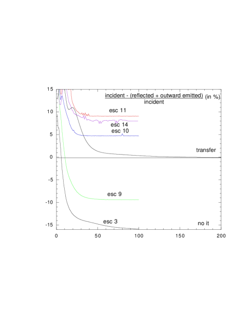
Figure 1: This figure shows the total net energy balance for the reference model, i.e. the difference between the total incident flux and the sum of the reflected and outward fluxes, referred to the incident flux, as a function of the number of iterations, with the different approximations and with the full transfer treatment. We do not show Escape 12, which converges towards +47$\%$, and Escape 13, which gives almost the same result as Escape 14. It shows that a large number of iterations are necessary for the convergence of Titan, which reaches then total energy balance, while the escape probability approximations converge more rapidly, but do not reach energy balance.

4 Escape probability versus transfer models

4.1 The models and the approximations used

Our reference model is a plane-parallel slab of constant density $n=10^{12}$ cm^-3 and total hydrogen column density $5\times 10^{24}$ cm^-2 (Thomson thickness $\tau_{es}=4$), irradiated on one side by a semi-isotropic incident continuum with a spectral distribution $F_{\nu}\propto\nu^{-1}$ extending from 0.1 eV to 100 keV. The ionization parameter $\xi$ at the surface of the irradiated slab, defined as $\xi=4\pi\ F/n$, where $F$ is the integrated incident flux and $n$ is the number density, is equal to $10^{3}$. The equilibrium temperature in such a slab (see below) varies between 10⁵ to 10⁶ K, so such a model is typical for the region emitting the “Big Blue Bump” in AGN, and for the “irradiated skin” of an accretion disc giving rise to the reflection spectrum observed in the X-ray range (Nayakshin et al. 2000). We also considered a thinner slab (column density $10^{24}$ cm^-2, i.e. $\tau_{es}\sim 1$) to see whether the escape approximation is more valid in this case.

Finally it is worth noticing that, keeping the same ionization parameter, we did not succeed in running any escape approximation with a slab thicker than $\tau_{es}=5$ (the energy balance does not converge).

In order to compare the structure and the emission spectrum computed with the escape probability approximation and with a real line transfer, we performed computations using, on one side the recently updated version of the code Titan (cf. Coupé 2002 for the atomic data) coupled with the NOAR code as described in DAC, plus ALI, and on the other side the same version (same atomic data, same transfer treatment of the continuum), but with the escape probabilities replacing the corresponding terms in the statistical and ionization equilibrium equations, in the energy balance and in the emitted line fluxes.

We have constructed a set of approximations. We give here neither the description nor the results corresponding to all our computations, but only those of the most representative ones, which follow as closely as possible the treatment of Ko & Kallman (1994), of Kallman & Bautista (2001), i.e. XSTAR, and of Ross-Ballantyne’s and Nayakshin’s codes.

Figure 2: Temperature versus $\tau_{es}$ for the reference model, with the different approximations and with the full transfer computation. The escape approximations give almost the same result as the transfer in the hot layers, but not in the colder ones.

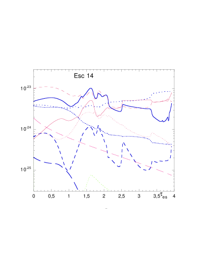
Figure 3: Heating and cooling rates due to the different processes, in ergs cm⁺³ s^-1, versus $\tau_{es}$, for the reference model, with the full transfer computation and with Escape 14 approximation. Thick lines correspond to cooling and thin lines to heating: solid lines: heating by photoionizations by line photons and net line cooling; large-dashed lines: Compton heating and cooling; small-dashed lines: heating by photoionizations due to continuum photons, cooling by radiative recombinations onto excited levels; very small dashed line: cooling by recombinations onto ground levels; dotted lines: free-free heating and cooling. We see that heating by line photons is much more important for $\tau_{es}\geq 2$ with the escape approximation than with the transfer treatment.

• Escape 3: line escape probability computed with Eqs. 21 and 2.2, energy balance with Eq. 33, line fluxes with Eq. 34, level populations with Eq. 29. This is a treatment similar to that of Ko & Kallman (1994), except that they consider a semi-infinite atmosphere, while we are considering a finite slab with escape from both sides. Also, we added a term of local ionization due to line photons:

  $$Ion=n_{u}A_{ul}\ P_{line}\times{\kappa_{c}\over\kappa_{0}+\kappa_{c}}$$ (38)

  and the corresponding energy gain term. Thus it is a pure local treatment.

• Escape 8: line escape probability computed with Eqs. 21 and 2.2, $P_{esc}$ computed with the Hummer operator, energy balance with only $P_{line}$ and line fluxes with Eq. 37, level populations with Eqs. 27 and 30. This treatment is similar to that of Kallman & Bautista (2001) with the exponential attenuation of the line photons towards the surface, and their non-local use for ionizations and gains of energy. The only difference is in the expression of the line escape probability (Eqs. 21 and 23 instead of Eq. 25).

• Escape 9: same as Escape 8, except that the line photons are taken into account in photo-absorption in both directions.

• Escape 10: same as Escape 8, except that the ionization and gain equations, $P_{esc}$ is replaced by $P^{{}^{\prime}}_{esc}$ of Kallman & Bautista (2001).

• Escape 11: same as Escape 9, except that the ionization and gain equations, $P_{esc}$ is replaced by $P^{{}^{\prime}}esc$ of Kallman & Bautista (2001).

• Escape 12: same as Escape 11, but using Eq. 3.1 as Kallman & Bautista (2001) for the escape probability.

• Escape 13: same as Escape 11, but using $\tau_{e}=\sqrt{3\tau_{abs}(\tau_{abs}+\tau_{es})}$ instead of $\sqrt{3}\tau_{abs}$ in the attenuation of the continuum photons. Note that the term $\sqrt{3}$ is present here to mimic our “semi-isotropic” treatment. Indeed Titan solves the transfer for a semi-isotropic radiation field, and in particular it considers an isotropic incident radiation, instead of a monodirectional intensity perpendicular to the surface as the other codes.

• Escape 14: same as Escape 13, but with $\tau_{0}$ replaced by $\sqrt{3}\tau_{0}$ in $P_{line}$ (Eqs. 21 and 23), to better fit the transfer treatment.

We have also tried an approximation identical to Escape 14 (Escape 14bis), except that the differential line fluxes are multiplied by a factor of two, which should be present to take into account the semi-isotropy of the radiation field. This approximation is therefore more rigorous, we will see however that it leads to stronger lines than the other approximations, much stronger than the full transfer computation. To clarify what we have done, we give in Appendix B more details about the full set of equations used in the last approximation, which we consider as being the best.

In summary, Escape 3 is close to the treatment of Ko & Kallman (1994), and is the only one to take into account for local escape by Compton diffusions in the statistical level equations, Escapes 8 and 10, 12, are close to that of Kallman & Bautista (2001) and of XSTAR, and Escape 11 and the following ones can be compared to the treatment of Ross-Ballantyne’s and Nayakshin’s codes. Since Escape 8 differs from Escape 10 exactly like Escape 9 differs from Escape 11, we do not show the results corresponding to this approximation.

4.2 Results: the structure

Table 1: Energy balance after convergence, for the reference model, with the different approximations and with the full transfer.

The computations performed with an escape probability approximation converge more rapidly than those with the full transfer. It was expected, since the lines require the convergence of only $\tau_{0}$ and $T_{tot}-\tau_{0}$ with the escape probability approximations. But this is actually only a “pseudo-convergence”, as the total energy balance, i.e. the difference between the incident flux and the emitted plus transmitted one, has a value different from zero. It is due to the reasons mentioned in the previous section. Fig. 1 displays this quantity referred to the incident flux (in percentage), as a function of the number of iterations. We see that the various approximations “converge” towards different values. From this point of view, the best approximation is Escape 10 (the balance is achieved within 5$\%$). Notice that Escape 3 is not completely “converged” after 100 iterations.

This absence of energy balance is linked with the discrepancy between the spectra, and in particular between the line fluxes, obtained in the case of the escape approximations and of the full transfer computation. To illustrate this fact, Table 1 gives the number of the approximation (column 1), the percentages of the line flux (reflected and outward) with respect to the incident flux (column 2), and the mismatch in energy balance in percents (column 3). With the transfer treatment, the spectral lines represent only 14$\%$ of the total emission, which we assume to be the correct value. We notice that the importance of the spectral lines is larger when the mismatch is larger and positive, indicating that it is partly due to the spectral lines. The other part is due to the continuum emitted outward.

The mismatch in energy balance has a relatively small influence on the structure in temperature $T$ in the hot layers, but not in the deepest layers (Fig. 2). This is because the energy balance is dominated by continuum processes, which are treated in the same way in the escape approximations and in the full transfer treatment. In the deepest layers, bound-bound transitions dominate both the cooling and the heating, owing to the smaller temperature, and the temperature equilibrium is therefore more sensitive to the approximation used.

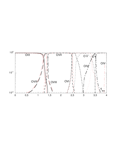
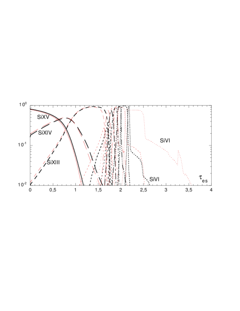
Figure 4: Fractional abundances of oxygen and silicium as functions of the optical thickness, for the reference model, with the full transfer computation (thick lines) and with Escape 14 approximation (thin lines). Ionization is strongly overestimated with the escape approximation for $\tau_{es}\geq 2$.

This can be seen in Fig. 3 which displays the local energy gains and losses due to the different processes for the full transfer computation and for Escape 14 approximation. One can also check that the “local energy balance” is achieved with a very good precision in all computations (actually better than 10^-4).

Though the losses and gains are quite similar in the transfer and in the escape treatment near the surface, one notices that in the region where $T$ is small (i.e. for $\tau_{es}\geq 2$), heating by photoionizations due to line photons, and line cooling, are important in the energy balance with the escape treatment. In particular the gains are dominated by photoionizations due to line photons, which are negligible in the transfer treatment. We will see later that X-ray line emissivities are overestimated in the escape treatment. It leads to the overestimation of photoionizations by line photons. Note in passing that lines of lithium-like ions have a role in the interplay between heating and cooling, and in the ionization equilibrium. First the medium is copiously cooled by lithium-like ions of elements like CNO, whose first excited levels have low potential energies (for this reason it is important to take into account carefully the excited levels of these ions). Second, owing to their relatively small ionization potential (for instance the ionization potential of OVI is 130 eV), they can easily be collisionally ionized at $T\sim 10^{5}$K.

As examples Fig. 4 displays the fractional abundances of oxygen and silicium as functions of the depth in the layer. Again the ionization equilibrium is little dependent on the approximation used near the surface, with the transfer and the escape treatments, but it is quite different in the deepest layers: the ionization state is overestimated in the escape treatment, and this is also linked to the overestimation of photoionization by line photons.

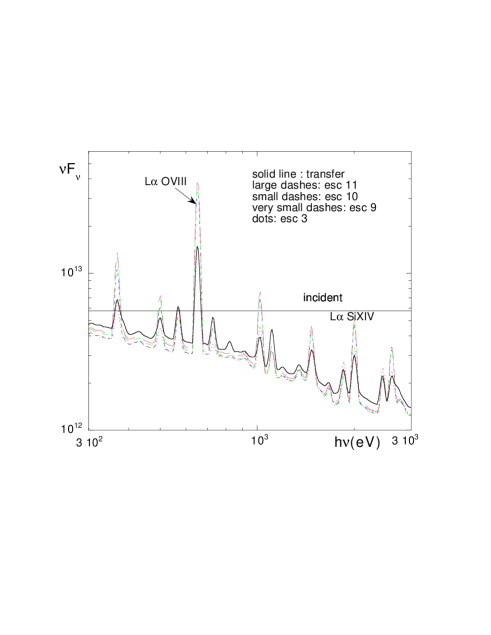
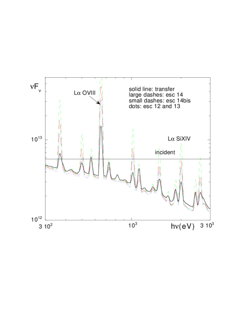
Figure 5: Reflected spectrum in ergs cm^-2 s^-1, for the reference model, with the different approximations and with the full transfer computation. The spectral resolution is 30.

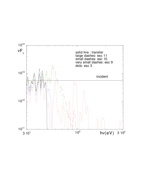
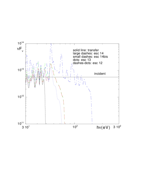
Figure 6: Outward emitted spectrum in ergs cm^-2 s^-1, for the reference model, with the different approximations and with the full transfer computation. The spectral resolution is 30. The flux is always overestimated with the approximations, owing to the overestimation of line ionization and heating in the deepest layers.

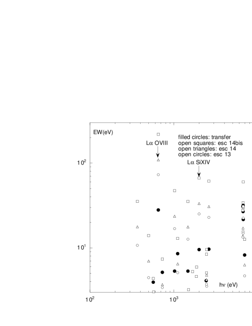
Figure 7: Line equivalent widths in eV, with respect to the total continuum (reflected plus incident), for the reference model, with the different approximations and with the full transfer computation. Some approximations lead to an overestimation of the EWs by one order of magnitude. Escape 3, which seems to be the best, gives weak lines because it overestimates continuum emission through the back side.The other approximations lead to at least a factor of three overestimation of the intense lines.

Figure 8: The reflected (solid line) and outward emitted (dotted line) spectra in ergs cm^-2 s^-1, with the full transfer computation: top panel: the reference model; bottom panel: the thin model. The spectral resolution is 30.

Figure 9: Reflected (top panel) and outward emitted (bottom panel) spectrum in ergs cm^-2 s^-1, for the thin model, with different approximations and with the full transfer computation. The spectral resolution is 30. The outward emitted spectrum is much better computed than in the case of the thicker slab, but still the lines are strongly overestimated.

4.3 Results: the spectrum

Figs. 5 and 6 display respectively the reflected and the outward emitted spectrum, in the full transfer and in the approximate computations. They are not intended to allow a detailed comparison, but only to show the broad differences between the results.

We first see that the reflected continua (Fig. 5) are very similar in all computations. This was expected as the structure in temperature and ionization of the hot part of the irradiated atmosphere is similar.

The outward emitted continua (Fig. 6) differ considerably in the UV and EUV ranges: it is due to the different ionization structure of the “cold” layers. With the transfer treatment the spectrum is completely cut above 54 eV, owing to the presence of a large fraction of He⁺ ions when $\tau_{es}\geq 3$, while with the escape probability approximations, helium remains completely ionized up to the back of the slab. It is particularly obvious for Escape 3 approximation, because the lines emitted by the surface layers are not reabsorbed by the continuum in the cold layers (note that Escape 3 is made for a semi-infinite medium). Escape 12 gives also a completely wrong outward spectrum, corresponding to the large mismatch in the energy balance.

Fig. 7 displays the equivalent widths in eV of the most intense lines, with respect to the total continuum (reflected plus incident - the outward emitted continuum is negligible in this frequency range), for the different approximations and for the transfer treatment. Strong discrepancies appear between the different escape approximations, and we see that basically they all lead to overestimates of the equivalent widths, sometimes by more than one order of magnitude. Note for instance the large value of the EW of the OVIII L$\alpha$ line at 650 eV with Escape 14 (220 eV), while it is only 28 eV with the transfer treatment. Note also that in the blend of iron lines near 7 keV, some lines are underestimated by the approximations, and other are overestimated, but they are not very different from the transfer treatment. Curiously, Escape 14bis, which is in principle the best approximation, give the worst results: the lines are in average 5-10 times more intense than with the transfer treatment, while this factor is only about 3 for the other approximations. Escapes 11 and 12 give exactly the same line spectrum, meaning that the approximation chosen for $P_{line}$ is actually not the dominant factor for the reflected spectrum, and that it is the treatment of the continuum absorption and of the Thomson scattering which plays the crucial role. The best approximation for the reflected lines is Escape 3, which is the worse for the outward spectrum! It is because the energy balance for this approximation is strongly negative, which is itself due to the fact that a large fraction of the radiation escapes from the back of the slab. On the other hand this approximation is the only one that takes into account Thomson-Compton scattering in the statistical equations, and we will see that it is in this respect better than the others.

We have not shown here the hard X-ray spectra: they are comparable with the escape approximations and with the transfer treatment. It is due to the similarity of the thermal state of the surface layers (cf. Fig. 2). For illustration, Fig. 8 (top panel) displays the whole reflected and outward emitted spectrum for the full transfer computation.

4.4 A “thin” model

To check whether the results would be better for the escape approximations with a thinner slab, we have run a model with a column density equal to $10^{24}$ cm^-2 (i.e. $\tau_{es}=0.8$). All the other parameters are identical to those of the reference model.

In this case the medium is almost homogeneous, with a temperature of the order of 1.5 10⁶ K in the whole slab. The escape probability approximations should therefore be more valid. It is only partly the case. The corresponding spectra are displayed on Fig. 9 for Escape 13, 14, and 14bis approximations. The agreement with the full transfer computation is indeed much better for the outward emitted continuum, but it is still very bad for the lines. Note in particular again the strong discrepancy of the OVIII L$\alpha$ line. It is due to the fact that in both the “thin” and the “thick” cases, the X-ray lines are formed in the same region $\tau_{es}\leq 1$, and the transfer suffers from the same problems, which will be discussed in the next section.

Fig. 8 (bottom panel) displays the whole reflected and outward emitted spectra for the full transfer computation, for this model.

5 Why are the line intensities larger with the escape approximations than with the full transfer treatment?

Figure 10: The differential reflected flux versus depth, for OVIII L$\alpha$ and SiXIV L$\alpha$ as a function of $\tau_{es}$, for the reference model with the different escape approximations. The solid line gives the value obtained with the full transfer treatment. We notice that the results have almost nothing in common, the transfer treatment leading to large negative values, which do not exist with the escape approximations, and which explain the overestimation of the line fluxes. The smaller line fluxes obtained with Escape 3 are actually due to the local treatment.

Figure 11: The product $\beta(ref)\times n_{2}$, proportional to the local line emissivity, as a function of $\tau_{es}$, for the reference model with the different escape approximations. The solid line gives the product $P_{e}(ref)\times n_{2}$, with $P_{e}(ref)$ defined in the text for the transfer treatment. Again the results are very different, with strong negative values in the case of the transfer treatment. The smaller value of the product with Escape 3 explains why the reflected fluxes are smaller.

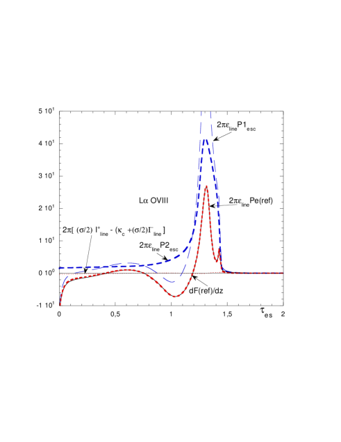
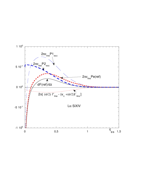
Figure 12: The different parts of the right member of Eq. 41, as functions of $\tau_{es}$, for the reference model, with the transfer treatment and for L$\alpha$ OVIII and SiXIV. It shows that for both lines (it is even more obvious for L$\alpha$ OVIII $),{dF(ref)/dz}$ is determined by $P_{e}(ref)$. $P_{e}(ref)$ itself is the difference of the two terms $P1_{esc}$ and $P2_{esc}$. The figure shows that the negative values of $P_{e}(ref)$ (and of $dF_{(}ref)/dz$) are due to the presence of the term $P2_{esc}$, i.e. to excitations by the diffuse continuum.

We would like to know whether the line intensities differ as a consequence of the local treatments, or of the treatments of the photons during their travel towards the surface, or both. It is not easy, because in the case of the transfer, local and non-local photons are not distinguishable.

To study the problem, we have chosen to examine two intense X-ray lines formed in different layers, OVIII L$\alpha$ and at 650 eV and SiXIV L$\alpha$ at 2 keV.

First it is necessary to know where these lines are formed. Note that the emission of both lines is restricted to the reflected flux. The differential reflected flux $dF_{ref}/dz$ is given by Eq. 49 for Escape 14, and one has equivalent expressions for the other escape approximations. For the transfer treatment, one cannot use directly Eqs. 2 or 18, because they give the flux in both directions, while we want only the reflected flux. In the two-stream approximation, the transfer equation becomes:

$${1\over\sqrt{3}}{dI_{\nu}^{+}\over dz} = -(\kappa_{\nu}+{\sigma\over 2})I_{\nu}^{+}+{\sigma\over 2}I_{\nu}^{-}+\epsilon_{\nu}$$ (39)

$${-1\over\sqrt{3}}{dI_{\nu}^{-}\over dz} = -(\kappa_{\nu}+{\sigma\over 2})I_{\nu}^{-}+{\sigma\over 2}I_{\nu}^{+}+\epsilon_{\nu}$$

where $I_{\nu}^{-}$ and $I_{\nu}^{+}$ are the intensities towards the surface and towards the back, and $F_{\nu}={2\pi/\sqrt{3}}(I_{\nu}^{+}-I_{\nu}^{-})$. The reflected flux integrated on the line profile can be obtained from these equations, like Eq. 2 was obtained from Eq. 2:

$${dF_{line}(ref)\over dz}={2\pi\over\sqrt{3}}{dI^{-}_{line}\over dz}=$$ (40)

$$\left[2\pi\epsilon_{line}-2\pi\kappa_{line}\int\phi_{\nu}I^{-}_{\nu}d\nu\right]$$

$$-2\pi(\kappa_{c}+{\sigma\over 2})I^{-}_{line}+2\pi{\sigma\over 2}I^{+}_{line},$$

where $I^{-}_{line}$ and $I^{+}_{line}$ are integrated on the line ($I_{line}=\int(I_{\nu}-I_{c})d\nu$), and $\int\phi_{\nu}I^{-}_{\nu}d\nu$ takes into account the continuum intensity $I^{-}_{c}$.

Fig. 10 shows ${dF_{line}(ref)/dz}$ for the two lines, as a function of the optical depth, for a few escape approximations and for the full transfer treatment. Actually there is almost nothing in common between the results of the two treatments! It is obvious that the smaller values of the line intensities with the transfer treatment come from the fact that ${dF_{line}(ref)/dz}$ is negative in a large fraction of the medium, while it is not the case in the escape treatment. This is due to the fact that the flux is directed towards the surface or towards the back, according to the variation of the source function (see below). Finally, one should note the much smaller flux obtained with Escape 3.

Note also that with the transfer treatment, the emission of OVIII L$\alpha$ is provided by a small layer located at $\tau_{es}\sim 1.3$. We have seen on Fig. 4 that it is precisely the region where OVIII ions are dominant. Thus we can infer that the emission is mainly due to excitation and not to recombination. Actually it is excitation by the diffuse continuum flux, and not by collisions. SiXIV emission is important up to $\tau_{es}\sim 1$, again when the SiXIV ions dominate, and SiXIV L$\alpha$ is also dominated by radiative excitation.

One can go a step further in our understanding. In analogy with Eq. 18, one can write Eq. 40:

$${dF_{line}(ref)\over dz}=2\pi\epsilon_{line}\times P_{e}(ref)+$$ (41)

$$-2\pi(\kappa_{c}+{\sigma\over 2})I^{-}_{line}+2\pi{\sigma\over 2}I^{+}_{line},$$

where

$$P_{e}(ref)={-2\pi\kappa_{line}\int\phi_{\nu}I^{-}_{\nu}d\nu+2\pi\epsilon_{line}\over 2\pi\epsilon_{line}}$$ (42)

is the equivalent of an escape probability for the reflected flux.

Fig. 11 displays the product $P_{e}(ref)\times n_{2}$, and compares it to $\beta(ref)\times n_{2}$ for different escape approximations ($\beta$ is given by Eq. 32). This last product is proportional to the local line emissivity with the escape approximations. Again there is little in common between the two treatments, but now we see that the reflected fluxes are determined by the local treatment, and not by the non-local one. This is in particular the case of Escape 3, which is the only local treatment to take into account Thomson-Compton scattering in the statistical equations (see below).

The second part of the right member of Eq. 41 is negligible, or at least not dominant, so the behavior of ${dF_{line}(ref)/dz}$ is determined by that of $P_{e}(ref)$. $P_{e}(ref)$ itself is the difference of two terms,

$$P1_{esc} = {-2\pi\kappa_{line}[\int\phi_{\nu}I^{-}_{\nu}(line)\ d\nu]+2\pi\epsilon_{line}\over 2\pi\epsilon_{line}}$$

$$= 1\ -\ {\int\phi_{\nu}I^{-}_{\nu}(line)\ d\nu\over S_{line}}$$

which can be identified with the one side escape probability computed with Eqs. 20 and 2.2, and a second term:

$$P2_{esc}={2\pi\kappa_{line}I^{-}_{c}\over 2\pi\epsilon_{line}}\ =\ {I^{-}_{c}\over S_{line}}$$ (44)

which corresponds to excitation of the line by the diffuse continuum, which is not taken into account in the expression of the escape probability.

Fig.12 shows $2\pi\epsilon_{line}P1_{esc}$ and $2\pi\epsilon_{line}P2_{esc}$. It proves that the negative values of $P_{e}(ref)$ and $dF_{line}(ref)/dz$ are mainly due to the diffuse continuum. It is a confirmation that the problem is mainly a local one, and does not depend much on the way the photons are treated non-locally in the escape approximations.

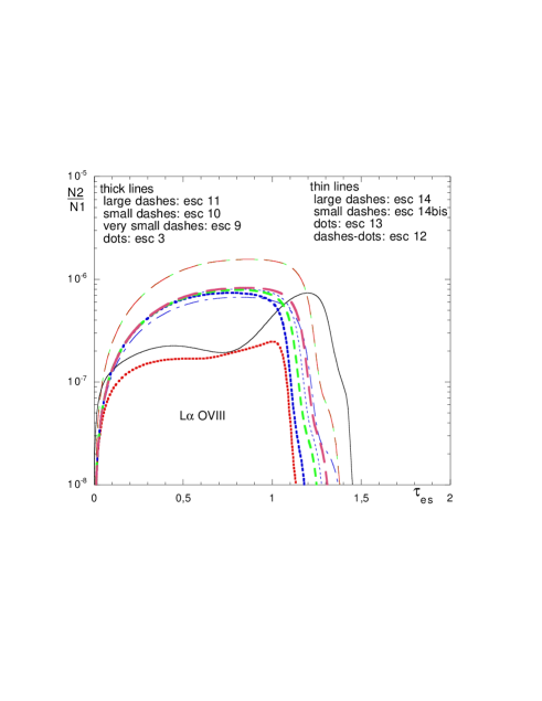
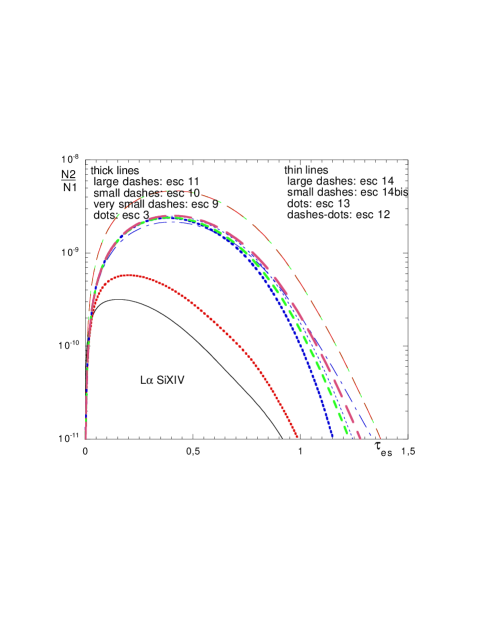
Figure 13: The ratio of the population of the upper level to that of the lower level, $n_{2}/n_{1}$ (proportional to the source function), for OVIII L$\alpha$ and SiXIV L$\alpha$, as a function of $\tau_{es}$, for the reference model with the different escape approximations. The solid line gives the ratio for the full transfer treatment. Except Escape 3, the other approximations strongly overestimate the source function, but Escape 3 underestimates it for the OVIII line in the region where it is emitted.

Figure 14: Comparison between the NRB and the escape probability $P_{esc}$ which replaces the NRB in the statistical equations of the levels computed with the escape probability, for OVIII L$\alpha$ and SiXIV L$\alpha$, as functions of $\tau_{es}$, for the reference model with the different escape approximations. The solid line gives NRB for the full transfer treatment. The escape approximations strongly underestimate $P_{esc}$, which means that they overestimate the importance of local diffusions. Escape 3 has a different behavior in this respect, because it allows the photons to escape by Thomson-Compton diffusions.

To stress this aspect, it is interesting to compare local quantities obtained with both treatments, such as the source function.

Fig. 13 displays the ratio of the population of the upper level to that of the lower level, $n_{2}/n_{1}$, which is proportional to the source function, for OVIII L$\alpha$ and SiXIV L$\alpha$, as a function of $\tau_{es}$. For both lines the source function is very badly determined by the escape approximations in the whole emission region, and it differs also by large factors between the different approximations, up to one order of magnitude. Except Escape 3, the other approximations mainly overestimate the source function. Escape 3 underestimates it for the OVIII line in the region where it is emitted. Since $n_{2}/n_{1}$ differs by large factors from the real value with the escape approximations, it means that any physical process implying the population of the upper level will be badly determined (we recall that the first levels have almost the same populations in all approximations, i.e. equal to the fractional abundances of OVIII and SiXIV).

Finally Fig. 14 displays the NRB and the escape probability $P_{esc}$ which is used instead of the NRB in the rate equations of the levels. There are large differences between the transfer treatment and the escape approximations, which are of course linked with the differences of the source function. Except Escape 3, the other approximations strongly underestimate $P_{esc}$, which means that they overestimate the importance of local diffusions. Escape 3 has a different behavior in this respect, because it allows the photons to escape by Thomson-Compton diffusions, but it is also bad in the region where the OVIII line is produced.

However the escape probability approximations do not overestimate all the lines. The lines which are most affected are those which have an intense underlying diffuse continuum. For the present model, it is not the case of the Fe lines near 7 KeV, because the diffuse continuum is relatively weak at this frequency. Therefore the Fe lines are computed relatively correctly by the approximations (within 30$\%$). It would probably be different with a very thick layer and a high ionization parameter. Again, we see that other models are required to set the limit of validity of the escape approximations.

6 Conclusion

In this paper we have shown that the escape probability approximations lead to a strong overestimation of the line intensities, in the case of a highly ionized and thick medium. They also lead to an overestimation of the ionization state at the back of the slab, and finally to an overestimation of the radiation escaping from the back.

We have shown that the local treatment is more important than the way absorption is taken into account non-locally. We have discovered that the much smaller values of the line intensities obtained with the transfer treatment are due to line excitations by the diffuse continuum, which are not taken into account correctly with the escape approximations. Considering the fact that the most correct expression for the emergent flux is that of Escape 14bis, which gives the largest line intensities (up to one order of magnitude larger than the full transfer treatment), it means that this process should be even more important than suspected. From this point of view the best approximation seems to be Escape 3, i.e. the one made by Ko and Kallman (1994), which includes a local escape from the line core by Thomson-Compton scattering in the statistical equations, but it is actually an artifact simply due to the fact that it reduces the source function in allowing this escape.

We stress also that the differences in the intensities of the X-ray lines between the various approximations on one hand, and between the escape approximations and the transfer treatment on the other hand, are almost exclusively due to the “transfer treatment”, as the structure of the hot part of the medium is almost the same in all cases, owing to the fact that the transfer of the continuum was perfomed exactly in the same way in all computations.

This result leads to the conclusion that not only the line transfer, but also the continuum transfer, should be correctly handled in order to get correct line intensities. In particular, it is not possible to use escape probability approximations to compute the diffuse continuum, as it is made in some codes.

This study was limited to one value of the ionization parameter ($\xi=1000$), and to a modest Thomson thickness. It has shown that the escape approximation is better in the case of a smaller thickness only for the emission from the back side. For the reflected line fluxes, it is equally bad, and we are inclined to think that only for Thomson thicknesses much smaller than unity, the escape probability approximations lead to correct X-ray line intensities in these hot media. We suspect that for a larger thickness, even the structure of the slab is badly computed. Note that the excitation equilibrium of the atoms is not correct. This can be important for denser media, where ionizations and line excitations can take place from excited levels. Thus it is mandatory to perform other comparisons in order to delineate the parameter region where the escape approximations can be used.

Finally it is worth mentioning that we have performed here all the computations assuming complete redistribution of frequencies, but with ALI it is equally possible to assume partial redistribution (cf. Paletou & Auer 1995), while this cannot be done with the escape formalism, unless very crude approximations are used.

APPENDIX A: Treatment of Comptonization in the lines by Titan

The transfer equation for the lines, in the absence of Compton scattering, can be written in the two-stream approximation:

$${1\over\sqrt{3}}{dI_{\nu}^{+}\over dz} = \ -(\kappa_{\nu}+\sigma)I_{\nu}^{+}+\sigma J_{\nu}+\epsilon_{\nu}$$ (45)

$${-1\over\sqrt{3}}{dI_{\nu}^{-}\over dz} = -(\kappa_{\nu}+\sigma)I_{\nu}^{-}+\sigma J_{\nu}+\epsilon_{\nu}$$

where $I_{\nu}^{+}$ and $I_{\nu}^{-}$ are respectively the outward and inward intensities.

During a Compton diffusion, a photon with an energy $E$ can lose an average energy $<\Delta E_{dc}>=E^{2}/mc^{2}$ for a direct Compton scattering, and gain an average energy $<\Delta E_{ic}>$ = $E\times 4kT/mc^{2}$ for an inverse Compton scattering. It is can be sent outside the Doppler core, provided that $|\Delta E_{dc}-\Delta E_{ic}|\geq cst\ \Delta\nu_{D}$, where $cst$ is of the order of unity, and $\Delta\nu_{D}$ is the Doppler width. It is then no longer absorbed inside the line.

In the transfer equation, we therefore treat differently the diffusion term $\sigma J_{\nu}$ for those photons which satisfy the previous condition (actually the value of $cst$ is not important): they are transferred like continuum photons. Their mean intensity is computed as:

$$J_{Compton}={\sigma\int J_{\nu}d\nu\over\Delta\nu_{Compton}},$$ (46)

where $\Delta\nu_{Compton}$ is set equal to:

$$\sqrt{\pi}\nu\sqrt{{2kT(0)\over mc^{2}}+{2\over 5}\left({h\nu\over mc^{2}}\right)^{2}}$$ (47)

where $T(0)$ is the surface temperature (actually $T$ is almost constant in the hot Comptonizing medium). These photons are taken into account like continuum photons in the heating and ionization equations. Conversely, continuum photons are injected in the line core by Compton scattering.

Comptonization in the lines is therefore now taken into account in the statistical equilibrium equations, in the transfer, and in the emerging line fluxes. The gains or losses corresponding to the Compton shift of line photons were already taken into account in the energy balance in the previous version of Titan.

APPENDIX B: Some details concerning Escape 14bis approximation

The local line cooling function is taken as:

$$\Lambda_{line}={n_{2}A_{21}h\nu\over n_{e}n_{H}}\times P_{escl}.$$ (48)

The reflected flux is computed as:

$$F_{ref}={1\over 2}\int{n_{2}A_{21}h\nu\beta^{\prime}_{ref}\ exp[-\tau_{e}]dz},$$ (49)

and the outward emitted flux is computed as:

$$F_{out}={1\over 2}\int{n_{2}A_{21}h\nu\beta^{\prime}_{out}\ exp[-T_{e}+\tau_{e})]dz},$$ (50)

where $T_{e}$ is the total optical thickness of the slab. $\beta^{\prime}_{ref}=P_{line}(\tau)+{1\over 2}(1-P_{escl}(\tau)){\sigma\over\kappa_{l}\sqrt{\pi}+\kappa_{c}+\sigma}$, and $\beta^{\prime}_{out}=P_{line}(T-\tau)+{1\over 2}(1-P_{escl}(\tau)){\sigma\over\kappa_{l}\sqrt{\pi}+\kappa_{c}+\sigma}$. $\tau_{e}$ is the effective continuum optical thicknesses in the two-stream approximation ($\tau_{e}=\sqrt{3\tau_{abs}(\tau_{abs}+\tau_{dif})}$).

The ionization rate $\kappa_{c}4\pi J_{l}/h\nu$ due to the lines, at the depth $z$, is equal to:

$$\kappa_{c}A_{21}\times{\bf[}\int_{0}^{z}{n_{2}(Z)\beta^{\prime}_{out}(Z)exp(-\tau_{e}(z)+\tau_{e}(Z))dZ}$$ (51)

$$+\int_{H}^{z}{n_{2}(Z)\beta^{\prime}_{ref}(Z)exp(-\tau_{e}(H)+\tau_{e}(Z))dZ}{\bf]},$$

where $H$ is the geometrical thickness of the slab. This expression is used for the gains by photoionizations due to the lines.

References

- (1) uer L.H., 1991, in: Stellar Atmospheres: Beyond Classical Models, Proceedings of the Advanced Research Workshop, Trieste, Italy, Dordrecht, D. Reidel Publishing Co.
- (2) Auer, L.H., Paletou, F. 1994, A&A, 284, 675
- Ballantyne, Ross, & Fabian (2001) Ballantyne, D. R., Ross, R. R., & Fabian, A. C. 2001, MNRAS, 327, 10
- Bonilha et al. (1979) Bonilha, J. R. M., Ferch, R., Salpeter, E. E., Slater, G., & Noerdlinger, P. D. 1979, ApJ, 233, 649
- Branduardi-Raymont et al. (2001) Branduardi-Raymont, G., Sako, M., Kahn, S. M., Brinkman, A. C., Kaastra, J. S., & Page, M. J. 2001, A&A, 365, L140
- (6) Cannon C.J. 1973, J. Quant. Spectroscop. Radiat.Transfer, 13, 627
- Collin-Souffrin, Delache, Frisch, & Dumont (1981) Collin-Souffrin, S., Delache, P., Frisch, H., & Dumont, S. 1981, A&A, 104, 264
- Collin-Souffrin, Czerny, Dumont, & Zycki (1996) Collin-Souffrin, S., Czerny, B., Dumont, A.-M., & Zycki, P. T. 1996, A&A, 314, 393
- (9) Coupé, S., 2002, PhD thesis, Université de Lyon
- Dumont, Abrassart, & Collin (2000) Dumont, A.-M., Abrassart, A., & Collin, S. 2000, A&A, 357, 823 (DAC)
- Dumont & Collin (2001) Dumont, A. & Collin, S. 2001, ASP Conf. Ser. 247: Spectroscopic Challenges of Photoionized Plasmas, 231
- Dumont, Czerny, Collin, & Zycki (2002) Dumont, A.-M., Czerny, B., Collin, S., & Zycki, P. T. 2002, A&A, 387, 63
- (13) Elitzur, M., 1982, Review of Modern Physics, 54, 1125
- Ferland & Rees (1988) Ferland, G. J. & Rees, M. J. 1988, ApJ, 332, 141
- Hollenbach & McKee (1979) Hollenbach, D. & McKee, C. F. 1979, ApJS, 41, 555
- Hubeny, Agol, Blaes, & Krolik (2000) Hubeny, I., Agol, E., Blaes, O., & Krolik, J. H. 2000, ApJ, 533, 710
- Hubeny (2001) Hubeny, I. 2001, ASP Conf. Ser. 247: Spectroscopic Challenges of Photoionized Plasmas, 197
- Hubeny, Blaes, Krolik, & Agol (2001) Hubeny, I., Blaes, O., Krolik, J. H., & Agol, E. 2001, ApJ, 559, 680
- (19) Hummer, D.G., 1968, MNRAS, 138, 73
- (20) Hummer, D.G., Rybicki, G.B., 1970, 150, 419
- Hummer & Kunasz (1980) Hummer, D. G. & Kunasz, P. B. 1980, ApJ, 236, 609
- (22) Irons, F.E., 1978, MNRAS, 182, 705
- Ko & Kallman (1994) Ko, Y. & Kallman, T. R. 1994, ApJ, 431, 273
- (24) Kalkofen, W., 1984, “Methods in radiative transfer”, Cambridge University Press
- Kallman & Bautista (2001) Kallman, T. & Bautista, M. 2001, ApJS, 133, 221
- (26) Kunasz, P., & Auer, H. L., 1988, J. Quant. Spectroscop. Radiat. Transfer, 39, 67
- (27) Lee, J.C., et al. 2001, ApJ, 554, L13
- Nayakshin, Kazanas, & Kallman (2000) Nayakshin, S., Kazanas, D., & Kallman, T. R. 2000, ApJ, 537, 833
- Netzer, Elitzur, & Ferland (1985) Netzer, H., Elitzur, M., & Ferland, G. J. 1985, ApJ, 299, 752
- (30) Ng K. C. 1974, J. Chem. Phys., 61, 2680
- (31) Olson, G.L., Auer, L.H., Buchler, J.R., 1986, J. Quant. Spectroscop. Radiat. Transfer, 35, 431
- (32) Olson, G.L., & Kunasz, P.B., 1987, J. Quant. Spectroscop. Radiat. Transfer, 38, 325
- (33) Paletou, F., & Auer, L.H., 1995, A&A, 297, 771
- Péquignot et al. (2001) Péquignot, D. et al. 2001, ASP Conf. Ser. 247: Spectroscopic Challenges of Photoionized Plasmas, 533
- Rees, Netzer, & Ferland (1989) Rees, M. J., Netzer, H., & Ferland, G. J. 1989, ApJ, 347, 640
- (36) Rybicki, G.B., Hummer, D.G., 1983, ApJ, 274, 380
- (37) Rybicki, G.B. & Hummer, D.G., 1991, A&A, 245,171
- (38) Ross, R. R., Weaver, R., & McCray, R. 1978, ApJ, 219, 292
- (39) Ross, R. R. 1979, ApJ, 233, 334
- Ross & Fabian (1993) Ross, R. R. & Fabian, A. C. 1993, MNRAS, 261, 74
- Różańska, Dumont, Czerny, & Collin (2002) Różańska, A., Dumont, A.-M., Czerny, B., & Collin, S. 2002, MNRAS, 332, 799
- (42) Trujillo Bueno, j. & Fabiani Bendicho, 1995, ApJ, 455, 646