From Small-Scale Dynamo to Isotropic MHD Turbulence

Abstract

We consider the problem of incompressible, forced, nonhelical, homogeneous, isotropic MHD turbulence with no mean magnetic field. This problem is essentially different from the case with externally imposed uniform mean field. There is no scale-by-scale equipartition between magnetic and kinetic energies as would be the case for the Alfvén-wave turbulence. The isotropic MHD turbulence is the end state of the turbulent dynamo which generates folded fields with small-scale direction reversals. We propose that the statistics seen in numerical simulations of isotropic MHD turbulence could be explained as a superposition of these folded fields and Alfvén-like waves that propagate along the folds.

The term ’MHD turbulence’ embraces a number of turbulent regimes described by the MHD equations. Their physics can be very different depending on the Mach number, presence of external forcing and of mean magnetic field, flow helicity, relative magnitude of the velocity and magnetic-field diffusion coefficients, etc. Here we consider what is perhaps the oldest MHD turbulence problem dating back to Batchelor_dynamo: incompressible, randomly forced, nonhelical, homogeneous, isotropic MHD turbulence. No mean field is imposed, so all magnetic fields are fluctuations generated by the turbulent dynamo. We are primarily interested in the case of large magnetic Prandtl number ${\rm Pr}=\nu/\eta$ (the ratio of fluid viscosity to magnetic diffusivity), which is appropriate for the warm ISM and cluster plasmas. Numerical evidence suggests that the popular choice ${\rm Pr}=1$ is in many ways similar to the large-${\rm Pr}$ regime. ${\rm Pr}\gg 1$ implies that the resistive scale $\ell_{\eta}\sim{\rm Pr}^{-1/2}\ell_{\nu}$ is much smaller than the viscous scale $\ell_{\nu}$. Thus, the problem has two scale ranges: the hydrodynamic (Kolmogorov) inertial range $\ell_{0}\gg\ell\gg\ell_{\nu}\sim{\rm Re}^{-3/4}\ell_{0}$ ($\ell_{0}$ is the forcing scale) and the subviscous range $\ell_{\nu}\gg\ell\gg\ell_{\eta}$. This makes it very hard to simulate this regime numerically.

For a moment, let us consider the traditional view of the fully developed incompressible MHD turbulence in the presence of a strong externally imposed mean field. This view is based on the idea of Iroshnikov and Kraichnan_MHD that it is a turbulence of strongly interacting Alfvén-wave packets. Their phenomenology, modified by GS_strong to account for the anisotropy induced by the mean field, predicts steady-state spectra for magnetic and kinetic energies that are identical in the inertial range and have Kolmogorov $k^{-5/3}$ scaling. An essential feature of this description is that it implies scale-by-scale equipartition between magnetic and velocity fields: indeed, $\delta{\bf u}_{\bf k}=\delta{\bf B}_{\bf k}$ in an Alfvén wave. Numerics appear to confirm the Alfvénic equipartition picture provided there is an externally imposed strong mean field. The reader will find further details and references in Chandran’s review in these Proceedings.

Figure 1: Energy spectra in our simulations of isotropic MHD turbulence. Here ${\rm Re}_{\lambda}={\langle u^{2}\rangle}^{1/2}\lambda/\nu\sim{\rm Re}^{1/2}$, where $\lambda=\sqrt{5}\,(\langle|\nabla{\bf u}|^{2}\rangle/{\langle u^{2}\rangle})^{-1/2}$ is the Taylor microscale and ${\rm Re}$ the box Reynolds number.

In the case of zero mean field, it is tempting to argue that essentially the same description applies, except now it is the large-scale magnetic fluctuations that play the role of effective mean field along which smaller-scale Alfvén waves can propagate. This is, indeed, what has widely been assumed to be true. However, the numerical simulations of isotropic MHD turbulence tell a very different story. No scale-by-scale equipartition between kinetic and magnetic energies is observed numerically. There is a definite and very significant excess of magnetic energy at small scales. This holds true both for ${\rm Pr}>1$ and for ${\rm Pr}=1$ (figure 1). The trend is evident already at low resolutions and persists at the highest currently available resolution ($1024^{3}$, see Haugen_Brandenburg_Dobler and their paper in these Proceedings).

In order to understand what is going on, let us consider the genesis of the magnetic field in the isotropic MHD turbulence. As there is no mean field, all magnetic fields are fluctuations self-consistently generated by the small-scale turbulent dynamo. This type of dynamo is a fundamental mechanism that amplifies magnetic energy in sufficiently chaotic 3D flows with large enough magnetic Reynolds numbers (typically above 100) and ${\rm Pr}\geq 1$ (note that both the physics and the numerical evidence that apply to plasmas with ${\rm Pr}\ll 1$, e.g., stellar convective zones and protostellar discs, are very different: see SCMM_lowpr). The amplification is due to random stretching of the (nearly) frozen-in magnetic-field lines by the ambient velocity field. What sort of magnetic fields does the dynamo make? During the kinematic (weak-field) stage of the dynamo, the growth of the field is exponential in time (figure 2a) and the magnetic-energy spectrum is peaked at the resistive scale, $k_{\eta}\sim{\rm Pr}^{1/2}k_{\nu}$, and grows self-similarly (spectral profiles normalised by ${\langle B^{2}\rangle}$ are shown in figure 1; theory is due to Kazantsev; KA). The dynamo growth rate is of the order of the turnover rate of the viscous-scale eddies, which are the fastest in Kolmogorov turbulence.

Figure 2: From kinematic dynamo to nonlinear steady state: (a) evolution of magnetic and kinetic energies, (b) evolution of characteristic wave numbers. Here $k_{\lambda}=(\langle|\nabla{\bf u}|^{2}\rangle/{\langle u^{2}\rangle})^{1/2}=\sqrt{5}/\lambda$; $k_{\rm rms}$ and $k_{\parallel}$ are defined in the text.

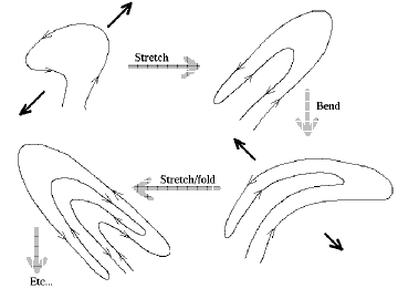
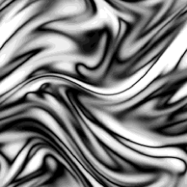
Thus, the bulk of the magnetic energy concentrates at the resistive scale. Let us inquire, however, what actually happens to the field lines? It turns out that the dynamo-generated fields are not at all randomly tangled, but rather organised in folds within which the fields remain straight up to the scale of the flow and reverse direction at the resistive scale. Figure 3b illustrates the folded structure observed numerically. Figure 3a explains how such fields result from repeated application of random shear to the field lines. The folded structure is, in fact, a measurable statistical property of the magnetic field. A variety of diagnostics can be used. Ott and coworkers noticed in early 1990s that kinematically generated fields exhibited extreme flux cancellation due to field reversals (see review by Ott_review). Our preferred description has been to compare the characteristic parallel and rms wave numbers of the field and to study the statistics of the field-line curvature (Kinney_etal; SCMM_folding, 2004c). We have shown that (i) $k_{\parallel}=(\langle|{\bf B}\cdot\nabla{\bf B}|^{2}\rangle/{\langle B^{4}\rangle})^{1/2}\sim k_{\nu}$ independently of ${\rm Pr}$ while $k_{\rm rms}=(\langle|\nabla{\bf B}|^{2}\rangle/{\langle B^{2}\rangle})\sim{\rm Pr}^{1/2}k_{\nu}\gg k_{\nu}$ (figure 2b) (ii) the bulk of the curvature PDF is at flow scales. This confirms the picture of direction-reversing fields that are straight up to the scale of the flow. Note that the folded structure is not static: it is a net statistical effect of constant restretching and partial resistive annihilation of the magnetic fields.

(a) (b)

Figure 3: The folded fields. (a) Sketch of the stretch-and-fold mechanism. (b) Cross-section of field strength in a simulation of nonlinear dynamo (${\rm Pr}=500$).

One immediate implication of the folded field structure is the criterion for the onset of nonlinearity: for incompressible MHD, the back reaction is controlled by the Lorentz tension force ${\bf B}\cdot\nabla{\bf B}\sim k_{\parallel}B^{2}$, which must be comparable to other terms in the momentum equation. This quantity depends on the parallel gradient of the field and does not know about direction reversals. Balancing ${\bf B}\cdot\nabla{\bf B}\sim{\bf u}\cdot\nabla{\bf u}$, we find that back reaction is important when magnetic energy becomes comparable to the energy of the viscous-scale eddies. Clearly, some form of nonlinear suppression of the stretching motions at the viscous scale must then occur. However, the eddies at larger scales are still more energetic than the magnetic field and continue to stretch it at their (slower) turnover rate. When the field energy reaches the energy of these eddies, they are also suppressed and it is the turn of yet larger and slower eddies to exercise dominant stretching. A model constructed along these lines Schekochihin et al. (2002b) leads us to expect a self-similar nonlinear-growth stage during which the magnetic energy grows $\propto t$ and the rms wavenumber of the magnetic field drops $\propto t^{-1/2}$ due to selective decay of the modes at the large-$k$ end of the magnetic-energy spectrum. The folded structure is preserved with folds elongating to the size $\ell_{\rm s}$ of the dominant stretching eddy. If ${\rm Pr}\gg\sqrt{{\rm Re}}$, the culmination of this process is a situation where total magnetic and kinetic energies are equal, ${\langle B^{2}\rangle}\sim{\langle u^{2}\rangle}$, the fields are still folded with $k_{\parallel}\sim$ inverse box size, and $k_{\rm rms}$ has dropped by a factor of ${\rm Re}^{1/4}$ compared to the kinematic case. Since ${\rm Pr}\gg\sqrt{{\rm Re}}$, we have $k_{\rm rms}\sim k_{\nu}{\rm Pr}^{1/2}{\rm Re}^{-1/4}\gg k_{\nu}$ still below the viscous scale. Thus, the condition ${\rm Pr}\gg\sqrt{{\rm Re}}$ is necessary for $k_{\rm rms}$ and $k_{\nu}$ to be distinguishable in the nonlinear regime. It is possible that a second period of selective decay ensues, but this cannot be checked numerically because the case ${\rm Pr}\gg\sqrt{{\rm Re}}\gg 1$ is unresolvable and likely to remain so for a long time. While astrophysical large-${\rm Pr}$ plasmas are certainly in this regime, the numerics can only handle $\sqrt{{\rm Re}}>{\rm Pr}\gtrsim 1$ (or ${\rm Pr}\gg\sqrt{{\rm Re}}\sim 1$, see SCTMM_stokes and figure 3b). What can we learn from such numerical experiments? Our model predicts that the nonlinear-growth stage in such a situation is curtailed with ${\langle B^{2}\rangle}/{\langle u^{2}\rangle}\sim{\rm Pr}/\sqrt{{\rm Re}}<1$ and magnetic energy residing around the viscous scale. Note that all these estimates are asymptotic ones, so factors of order unity can obscure comparison with simulations, in which only very moderate scale separations can be afforded. With this caveat, we claim that the numerically observed state where there is excess magnetic energy at small scales but overall ${\langle u^{2}\rangle}>{\langle B^{2}\rangle}$ (figure 1), is consistent with our prediction. The ratio ${\langle B^{2}\rangle}/{\langle u^{2}\rangle}$ does increase with ${\rm Pr}$, but a conclusive parameter scan is not yet possible. Furthermore, the reduction of $k_{\rm rms}$ in the nonlinear regime, as well as the elongation of the folds (decrease of $k_{\parallel}$), are clearly confirmed by the numerics (figure 2b).

Figure 4: Alfvén waves superimposed on folded fields.

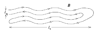
Our model was based on the assumption of some effective nonlinear suppression of stretching motions. This does not have to mean complete suppression of all turbulence in the inertial range. Two kinds of motions that do not amplify the field can, in principle, survive. First, the velocity gradients could become locally 2D and perpendicular to the field (a quantitative model based on such two-dimensionalisation is described in SCTHMM_aniso and SCTMM_stokes). One should expect a large amount of 2D mixing of the direction-reversing field lines leading to very fast diffusion of the field. If this happens, any selective decay must be ruled out, i.e., the nonlinear-growth stage cannot occur and ${\langle B^{2}\rangle}$ cannot grow above the viscous-eddy energy. Since numerics support selective decay and saturated values of ${\langle B^{2}\rangle}$ are certainly far above the energy of the viscous eddies, we tentatively conclude that mixing due to the surviving 2D motions is not very efficient. The second kind of allowed motions are Alfvén waves that propagate along the folded direction-reversing fields (figure 4). Their dispersion relation is $\omega_{\bf k}=\pm({{\hat{\bf b\mkern-4.0mu}\mkern 4.0mu}{}}{{\hat{\bf b\mkern-4.0mu}\mkern 4.0mu}{}}:{\bf k}{\bf k})^{1/2}{\langle B^{2}\rangle}^{1/2}$, where ${{\hat{\bf b\mkern-4.0mu}\mkern 4.0mu}{}}={\bf B}/B$ and $k$ varies between the inverse length of the folds ($\sim$ box size) and $k_{\nu}$ Schekochihin et al. (2002b). These waves do not stretch the field, do not know about the direction reversals, and have the same properties as standard Alfvén waves. However, Fourier transforming a field structure sketched in figure 4 would not give ${\bf B}_{\bf k}={\bf u}_{\bf k}$ (scale-by-scale equipartition). Instead, the magnetic-energy spectrum would be heavily shifted towards small scales due to the presence of direction reversals. The Alfvén-wave component, while mixed up with folds in the magnetic field, should be manifest in the velocity field. We therefore expect the kinetic energy to have an essentially Alfvénic spectrum, probably $k^{-5/3}$. This picture accounts for the excess small-scale magnetic energy observed in numerical simulations. Thus, we conjecture that the fully developed isotropic MHD turbulence is a superposition of Alfvén waves and folded fields. The advent of truly high-resolution numerical simulations should make it possible to confirm or vitiate this hypothesis in the near future.

A more extended exposition of the ideas presented above, as well as a detailed account of the numerical evidence, are given in an upcoming paper by SCTMM_stokes.