Far Ultraviolet Spectroscopic Explorer Survey of the Local Interstellar Medium within 200 Parsec
Abstract
We present Far Ultraviolet Spectroscopic Explorer observations of the interstellar gas toward 30 white dwarf and 1 subdwarf (SdO) stars. These sightlines probe the Local Bubble (LB) and the local interstellar medium (LISM) near the LB. We systematically measure the column densities for the following species: C II, C II*, C III, N I, N II, O I, Ar I, Si II, P II, Fe II, Fe III, and H2. Our survey detected only diffuse H2 molecular clouds () along six sightlines. There is no evidence from this study that H2 exists well inside the perimeter of the LB. The kinematical temperature for H2 is less than the usual temperature observed in the local interstellar clouds, implying different gas phases in the LISM. The relative abundance ratios of Si II, P II, and Fe II give insight about the dust content. These ratios vary, but are similar to the depletion patterns observed in warm and halo diffuse clouds in more distant sightlines in the Galaxy. The N I/O I and Ar I/O I ratios are significantly subsolar within the LB. Outside the LB a larger scatter is observed from subsolar to solar. Because Ar and N are only weakly depleted into dust grains if at all, the deficiencies of their neutral forms are likely due to photoionization. The evidence for significant ionization of N (and hence Ar) is strengthened by the detection and measurement of N II, which is a dominant ion for this element toward many sightlines. C III appears to be ubiquitous in the LISM toward our sightlines, but C II remains the dominant ionization stage of C. The limits on Fe III/Fe II imply that Fe II is the dominant ion. These observations imply that photoionization is the main ionization mechanism in the LISM and do not support the existence of a highly ionized condition in the past. In view of the variations observed in the different atomic and ionic ratios, the photoionization conditions vary significantly in the LB and the LISM. The cooling rate in the LISM, (in erg s-1 (H I atom)-1), derived from the emission of the C II 157.7 line has a mean value of dex, very similar to previous determinations.
1 Introduction
Because of its proximity, the local interstellar medium (LISM) provides an unique opportunity to study in detail the physics of the warm (partially ionized) interstellar gas. Such gas is a major component of the interstellar material in the Galaxy and in other galaxies. The overall characteristics (temperatures, densities, kinematics) of the LISM were determined with ground-based telescopes and the Copernicus, International Ultraviolet Explorer (IUE), the Hubble Space Telescope (HST) satellites (e.g., McClintock et al., 1975; Bruhweiler & Kondo, 1982; Frisch & York, 1983; Linsky et al., 1993; Lallement et al., 1995; Redfield et al., 2002). Measurements of interstellar gas after it has entered the heliosphere has also provided information on the interstellar medium very close to the sun (see, e.g., studies of the local interstellar cloud by Lallement 1998 and by Slavin & Frisch 2002 and references therein).
From the ground-based observations, via mainly the Ca II K and Na I D absorption lines, very accurate absolute wavelength and very high spectral resolution provide precise information on the local gas dynamics and the complex velocity structure of nearby gas (e.g., Vallerga et al., 1993; Ferlet, 1999, and references therein). UV resonance absorption lines are much stronger than the available optical absorption lines (which are not in the dominant ionization stages), and are therefore more sensitive probes of the warm, low density LISM. Major advances in determining the physical conditions have been carried-out with UV observations, especially in the last decade, with the Goddard High Resolution Spectrograph (GHRS) and the Space Telescope Imaging Spectrograph (STIS) onboard HST (e.g., Linsky et al., 1993; Lallement et al., 1995; Lallement, 1996; Linsky, 1996).
With high spectral resolution ultraviolet observations, the physical properties of the cloud surrounding our solar system (the local interstellar cloud, LIC) can be estimated. The LIC is not very dense ( cm-3), but it is warm ( K) and partially ionized (e.g., Frisch & York, 1983; Lallement, 1996; Linsky, 1996). Near the LIC, there are similar clouds with different velocities (see, Linsky et al., 2000). All these clouds constitute collectively the LISM, and the clouds within roughly 100 pc are in a region called the Local Bubble (LB; the cavity has a radius of about 100 pc in almost every direction, except toward one very low column density direction ( CMa) where it extends to 200 pc; Sfeir et al. 1999). Na I absorption line studies by Sfeir et al. (1999) show that the boundary of the LB is delineated by a sharp gradient in the neutral gas column density with increasing radius. The distance of this boundary deduced from X-ray data is generally smaller by about 30% (see Snowden et al. 1998). In this study, we use the Far Ultraviolet Spectroscopic Explorer (FUSE) satellite to survey sightlines with distances less than 200 pc. For the purposes of this study, this distance will define the extent of the LISM. Even though the distances are not great in the LISM, the sightlines are expected usually to have complex kinematical structure (e.g., Lallement et al., 1995).
EUVE observations also have improved our knowledge of the ionization structure of the LISM (see the review by Bowyer, Drake, & Vennes, 2000, and references therein). The EUVE data show that the neutral helium to neutral hydrogen ratio is about 0.07, which is somewhat less than the cosmic abundance of He to H of 0.1 (Dupuis et al., 1995). Helium is therefore more ionized than H. Also, He shows less variability in its degree of ionization from one region to the next (Wolff, Koester, & Lallement, 1999). One possible explanation for the high fractional ionization of He in the LISM is that there has not been enough time for the ionized He to recombine to an equilibrium concentration from a more highly ionized condition in the past, perhaps from the influence of radiation from a supernova or its shockwave less than few years ago (Frisch & Slavin, 1996; Lyu & Bruhweiler, 1996). A different alternative is that the LISM is currently exposed to a strong, steady flux of photons with eV (e.g., a conductive interface between the LISM and a surrounding medium at K; Slavin & Frisch 2002, or by recombination radiation from highly ionized but cool gases; Breitschwerdt & Schmutzler 1994). A way to distinguish between these possibilities is to study the lightly depleted elements Ar, N, and O (Sofia & Jenkins, 1998). In particular, the ionization of Ar (and to a lesser extent of N) can help us to differentiate between photoionization equilibrium and non-equilibrium cooling models.
It is possible to increase our knowledge of the ionization structure of the LISM significantly by using data from FUSE (Jenkins et al., 2000; Lehner et al., 2002; Moos et al., 2002; Wood et al., 2002b). For instance, Jenkins et al. (2000) found a deficiency of Ar I toward 4 white dwarf (WD) stars, thus favoring photoionization equilibrium. In the present work, we increase the sample to 31 stars that are located within 200 pc. WDs are particularly good background objects for studying the LISM because they are nearby, they have relatively simple stellar continua, and they are often nearly featureless. FUSE gives access to the wavelength interval between 905 Å and 1187 Å, a region containing features of some important neutral species (N I, O I, and Ar I), many ionized species (C II, C III, N II, P II, Fe II, and Fe III), and H2. Surveys of O VI interstellar absorption and D I/O I ratio will be discussed by Oegerle et al. (2003) and Hébrard et al. (2003), respectively. Although FUSE has a moderate resolution of and, hence, only the properties of the dominant cloud or the “average” properties of the clouds can be derived, the large number of resonance lines for atoms in several ionization stages as well as molecular lines provides the unique opportunity to study in detail the ionization structure, dust, and molecules in the LISM.
2 Observations
2.1 The Sample
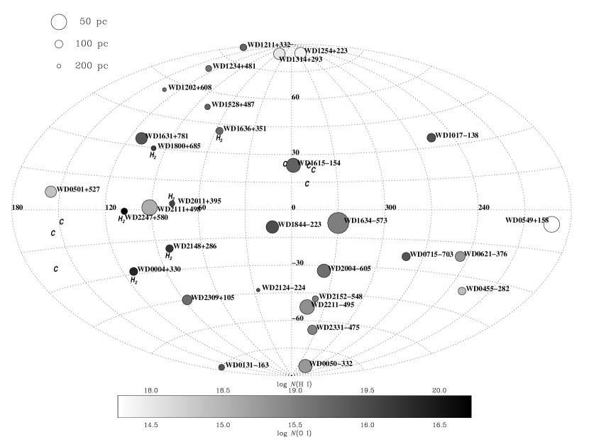
In Table 1, we list the positions, spectral types, distances, and heliocentric velocities for the sample of 31 stars observed with FUSE. The distribution of the targets on the sky is shown in Galactic coordinates in Figure 1. There is a good coverage of the sky in almost each quadrant with the exception of the region spanned by and . Most of the WDs are from the FUSE PI Team programs (P104 and P204) used to study D/H and O VI in the LISM. The primary criterion for selecting the stars in Table 1 was that we would be able to measure the species of interest for this work (see § 3) with a sufficient degree of confidence.
Recently, in the course of the FUSE observatory program “Survey of White Dwarfs from the McCook and Sion Survey” (Z903), several other WDs were observed. The quality of these data are not good enough for this study because strong airglow emission lines are present at all wavelengths and the signal-to-noise levels are too low (the flux of these WDs in this program are systematically lower than in the PI team programs). We also note that these targets do not fill in the deficiency of targets in the quadrant at , .
2.2 Instrument and data reduction
The FUSE instrument consists of four channels: two optimized for the short wavelengths (SiC 1 and SiC 2; 905–1100 Å) and two optimized for longer wavelengths (LiF 1 and LiF 2; 1000–1187 Å). There is, however, overlap between the different channels, and, generally, a transition appears in at least two different channels. More complete descriptions of the design and performance of the FUSE spectrograph are given by Moos et al. (2000) and Sahnow et al. (2000). To maintain optimal spectral resolution the individual channels were not co-added together. Also, measurements on the independent spectra could be compared with each other to obtain information about the effects of detector fixed pattern noise. Detailed information for each sightline, including whether the low resolution (LWRS) apertures or the medium resolution (MDRS) apertures were used, can be found in Table 1.
Standard processing with the current version of the calibration pipeline software (version 2.0.5 and higher) was used to extract and calibrate the spectra. The software screened the data for valid photon events, removed burst events, corrected for geometrical distortions, spectral motions, satellite orbital motions, and detector background noise, and finally applied flux and wavelength calibrations. The extracted spectra associated with the separate exposures were aligned by cross-correlating the positions of absorption lines, and then co-added. In some cases, the lack of strong absorption lines or the contamination of airglow lines prevented us from determining the relative displacements, so we simply coadded the spectra with no shifts. Generally, the different exposures were obtained successively, so no large shifts were expected and no significant loss of spectral resolution was observed. The co-added spectra were finally rebinned by 4 pixels ( mÅ) since the extracted data are oversampled.
Figure 2 presents two examples of FUSE calibrated spectra of WDs. As can be seen in the figure, the stellar continua are relatively simple and can be fitted with low-order () Legendre polynomials. The primary error sources are statistical noise, fixed-pattern noise, and possible saturation effects in the lines. The fixed-pattern noise is reduced by comparing the same spectral feature in different channels, while saturation can be examined when there are several transitions of the same species with different values (§ 3).
3 Spectral Features
3.1 General Considerations
The primary objective of this work is to measure the column densities of the neutral atoms, weakly ionized atoms and molecular hydrogen toward sightlines within 200 pc in order to probe the physical conditions within the LISM. For such study FUSE provides access to several important resonance lines, and we have measured systematically the column densities, , (or limits on the column densities) for the following species: C II, C II*, C III, O I, N I, N II, Si II, P II, Ar I, Fe II, and Fe III. The column densities of H2 were determined by using the Lyman and Werner bands. We note that P III and N III also are present in the FUSE bandpass and are potentially interesting ions. However, the P III transition is too weak to be detected and its 3 upper limit does not constrain the ratio P II/P III in a meaningful way. N III is blended with the saturated Si II line and possibly with photospheric N III making any measurements of this line highly uncertain. However, upper limits obtained by assuming that N III is not blended and lies on the linear part of the curve of growth (COG) show that N III is not the dominant ion stage of N in the LISM. Corrections for saturation would increase the upper limit, but this effect is likely less than the contribution from the Si II blend. Therefore, nitrogen is primarily N I and N II in the LISM.
In Table 2, we summarize the atomic/ionic transitions used in this work. To measure the column densities (see below), we adopted wavelengths and oscillator strengths from the Morton (2000, private communication) atomic data compilation. This compilation is similar to the Morton (1991) compilation with only a few minor updates to the atomic parameters for lines of interest in this study. For the Fe II lines, the new oscillator strengths derived by Howk et al. (2000) were adopted. We note, however, that there is a new laboratory measurement of the -value for Fe II 1144.9 (, Wiese, Bonvallet, & Lawler, 2002), which is about 30% lower than the experimental value of Howk et al. (2000). However, Wiese, Bonvallet, & Lawler (2002) note that additional study is necessary for the other transitions available in the FUSE bandpass, rather than a simple rescaling, as they are further down on the COG than the Fe II 1144.9 line. As we use all the transitions available in the FUSE spectrum, we employ the -values of Howk et al. (2000).
3.2 Photospheric Lines
To varying degrees, WD stars have sharp metal photospheric lines that can mimic interstellar lines, and therefore it is important to identify and disentangle them. Some WDs can be pure hydrogen (no photospheric metal lines) and some have only small amounts of metals in their photosphere. Their metallicity is generally very sub-solar (less than a few solar metallicity, ), and only a few metal-rich WDs are as high as (e.g., WD 2211495, WD 0621376). As a consequence, WDs have relatively smooth continua with only a few stellar lines. Figure 2 presents spectra of two WDs, one pure hydrogen and the other with some metals, with the interstellar lines flagged. Table 1 summarizes the metallicity of the WDs.
The lines that can be affected by photospheric lines are C III 977, Ar I 1066, P II 1052, and Fe III 1122. C III can be present in WDs with K, and peak at K (see Chayer, Fontaine, & Wesemael, 1995). Thus, when the star is not pure hydrogen, some contamination is expected for C III. Generally the stellar radial velocity is not different enough from the interstellar component to be able to distinguish between the two components. Photospheric Fe III can be also present for WDs with K. Moreover, Fe III 1122.53 is blended with photospheric Si IV 1122.49. For this species, we have a direct diagnostic for knowing if there is photospheric Si IV 1122 or Fe III 1122 by inspecting the lines Si IV 1128 and Fe III 1128 (see Figure 2 in Chayer et al., 2000). P II and Ar I are not found in the photosphere of the WDs, but can be blended with Fe VI, Ni VI 1152 and Si IV 1066, respectively. Fe VI (and Ni VI) are present in significant quantities only at K (Chayer, Fontaine, & Wesemael, 1995). Therefore for most of our sample, these blends with Fe VI and Ni VI are not much of a concern. For Si IV 1066 we look at longer wavelengths (e.g. Si IV 1128) for possible presence of this line. We finally note that some of the N I, O I, Fe II, and H2 transitions may be blended with some stellar lines, but the (generally) large numbers of transitions for these species allow us to detect if a specific line is contaminated.
3.3 Circumstellar Lines
Our survey used hot WDs, typically with temperatures ranging from 30,000 to 70,000 K (the subdwarf SdO BD+28°4211 has a temperature of 82,000 K; Sonneborn et al. 2002). Such hot WDs are emitting a large number of ionizing ultraviolet photons, creating Strömgren spheres with radii from 8 upto 30 pc depending on the electron density and the temperature of the WD (Dupree & Raymond, 1983; Tat & Terzian, 1999). Bannister et al. (2003) recently found direct evidences of such circumstellar absorption features (in form of high ions such as C IV) in the spectra of 4 WDs out of 11 present in our survey. Therefore, our study of the ionization conditions in the LISM could a priori be systematically biased because of the use of hot WDs. However, to probe these conditions, we employ mainly diagnostics from neutral species, such as N I, O I, and Ar I, species not present in the completly ionized Strömgren spheres. We have found no correlation between the ratios of Ar I/O I and N I/O I with the temperature of the WDs. While it is clear that the hot WDs participate to the overall ionization of the LISM (Vallerga, 1998; Slavin & Frisch, 2002), we have no evidence that stronger EUV sources give different results compared to weaker EUV sources in our column density ratios.
3.4 Geocoronal Emission Lines
Contamination of the spectra by geocoronal emission can be significant for the LWRS apertures of the FUSE spectrograph. Such emission lines are very strong at H I Ly , but decline rapidly in strength for the higher Lyman lines. During the sunlit part of the orbit, airglow emission lines are also present for many of the same lines of N I, O I, and Ar I used to measure the absorption by interstellar species. The importance of airglow emissions depends on many factors, including the fraction of sunlit time, the limb angle, the flux of the target, the aperture used, and the length of individual exposures. For the stars considered in this study, the observational strategy was to reduce the contribution from airglow lines: (1) The targets were observed in a manner that maximized the night time fraction, ranging typically from 30% to 100% (only WD 1234+481 was observed with basically no night time). (2) In order to remove small spectral shifts during an observation caused by thermally induced motion of the optics, an exposure is broken up into a large number of sub-exposures. Correlation techniques using uncontaminated interstellar lines are used to remove the shifts between the spectra and they are then added. To the extent the shifts are due to telescope mirror motions rather than grating motions, these shifts will smear out the airglow contribution. In practice, impact of the airglow contamination is reduced by this technique. (3) The objects studied are relatively bright with fluxes from a few to erg cm-2 s-1 Å-1. (In contrast the stars from the Z903 program have lower fluxes, long individual exposure times, and are observed largely in day time.) However, even under the conditions mentioned above, the airglow could still be significant. Therefore, we took several steps discussed below to check for possible contamination.
The widths of the airglow lines are determined by the size of the spectrograph apertures. For the LWRS aperture, the width of an airglow is typically 0.35 Å, while it is typically 0.045 Å for the MDRS aperture. Figure 2 illustrates the differences in strength and width of the airglow lines between the MDRS aperture (WD 1800+685, night fraction of 0.85) and LWRS aperture (WD 0131163, night fraction of 0.95). Hence with the LWRS aperture, the primary concern for measuring the interstellar lines considered here is the continuum placement, but for the MDRS aperture, the width is small enough that the emission could fill the interstellar lines. Several of our targets were observed with both the LWRS and MDRS apertures. The column densities generally agree within the errors, and in particular there was no systematic smaller column densities derived with the MDRS compared to those derived with the LWRS.
Feldman et al. (2001) have reported the brightnesses of the terrestrial day airglow lines using the FUSE instrument. We have examined airglow lines not blended with interstellar lines to estimate if our interstellar measurements could suffer from airglow contamination. At Å, we use the O I 1D–1D0 1152 line as an indicator for the presence of N I emission near 1134 Å, since the lines have comparable strengths. This airglow line can cause a continuum placement problem for the measurement of P II 1152 as shown in Figure 2 in the spectrum of WD 0131163. We were careful to use the N I 1134 lines only when these lines were not contaminated by airglow. At Å, we checked the strengths of several O I airglow lines at 1027, 1028 and 1042 Å. These lines have strengths that indicate the strengths of the O I 1039 and Ar I 1048, 1066 airglow lines. We do not find any cases where the contamination could be troublesome (in any case the 1 errors quoted here should be larger than the effects of contamination). Finally, at Å, where the most useful lines of N I and O I are located, the airglow emissions are negligible based on O I 990. Generally, we are confident that the airglow lines do not seriously compromise our interstellar measurements in ways we do not recognize.
3.5 Interstellar Absorption Lines
3.5.1 Species with Only One or Two Transitions
The apparent optical depth (AOD) method (Savage & Sembach, 1991) was used when only one or two lines of the same atomic species were available. The absorption profiles were converted into apparent optical depths per unit velocity, , where , are the intensity without and with the absorption, respectively. is related to the apparent column density per unit velocity, (cm-2 ()-1) through the relation . The integrated apparent column density is equivalent to the true integrated column density in cases where the absorption is weak () or the lines are resolved. This method was also used to place a lower limit on a saturated line.
For C II and N II, only a strong transition is available, and therefore, except for a few cases, the column densities are lower limits. The P II transition is weak for all of the sightlines considered. C II* is also usually relatively weak for the sightlines considered, but can be slightly blended with the Lyman 5–0 R(1) line of H2. When hydrogen molecules are present along a sightline, the contribution of both lines can still be measured because the shift between the two lines is large enough.
Si II has two transitions. The weakest one is free of blending with other interstellar or stellar lines, but the strongest transition at 989.873 Å is usually saturated and blended with N III of interstellar or stellar origin.
For Ar I, two transitions are also available at 1048.22 and 1066.66 Å, with the latter being the weakest transition of the two. We can therefore check for the effect of saturation, except when the WD is not pure hydrogen in which case Ar I 1066.66 is blended with the stellar Si IV 1066.66.
3.5.2 Species with several () transitions: N I, O I, Fe II, and H2
A COG analysis was undertaken when several lines were present (N I, O I, Fe II, and H2) by using the measured equivalent widths. The equivalent widths were measured by directly integrating the intensity, and their errors were derived following the method described by Sembach & Savage (1992). A single component Gaussian (Maxwellian) curve of growth was constructed in which the Doppler parameter and the column density were varied to minimize the between the observed equivalent widths and a model curve of growth. For H2, first a COG was constructed for the set of lines within each rotational level (). The resulting column densities and -values were then used as the starting point for a minimization of a COG that simultaneously included all of the rotational levels with the column density for each level and a single value as free parameters.
Depending on the quality of the data and the amount of matter along a given sightline, we found that generally the column densities of N I, O I, and Fe II were well determined with a COG because they have several transitions with different in the FUSE bandpass. We found that fixed-pattern noise was not a serious problem, and the effects of saturation can be reasonably well understood. In Table 3, we compare the -values of N I and O I obtained from the COG analysis, and within the errors, they are generally similar. In isolated cases where there was no good constraint on , we used the -value from one species to constrain the column density of the other. Those cases are indicated by colons in Table 3. The different Fe II transitions generally lie on the linear part of the COG.
Even though we considered seriously the saturation problem, with the FUSE spectral resolution, it still could be that narrow, unresolved components could be concealed by broader features. Jenkins (1986) showed, however, that column densities remain accurate to 10% provided that the lines are not heavily saturated (central optical depth such as ) and and do not have a bimodal distribution function. Three sightlines (WD 0501527, WD 1254223, and WD 1314293) of our sample were obtained with high spectral resolution using STIS. Redfield & Linsky (2003), but see also Vidal-Madjar et al. (1998) and Kruk et al. (2002), derived the column densities of several species considered in our survey for these sightlines, and their total column density measurements are in agreement within 1 with ours. This shows that FUSE measurements are reliable despite the moderate spectral resolution of the instrument. It also shows that the oscillator strengths of the species available in the FUSE wavelengths are also reliable.
3.5.3 Upper Limits
The upper limits for the equivalent widths are defined as , where is the inverse of the continuum S/N ratio per resolution element Å FWHM. The corresponding upper limits on the column density, presented in Table 4, are obtained from the corresponding equivalent width limits and the assumption of a linear curve of growth.
3.6 Results from Other Sources
Table 1 lists the sources of the column densities when they were derived from other investigations. For the sightlines that are reported in the ApJS special issue on the determination of D/H with FUSE (Hébrard et al., 2003; Kruk et al., 2002; Lehner et al., 2002; Lemoine et al., 2002; Sonneborn et al., 2002; Wood et al., 2002a), we complemented the measurements with additional measurements of the column densities for species considered here but not in those papers. In addition, for WD 1631781 and WD 2004-605, the values reported here are a mean between our methods (AOD and COG) and the profile fitting method reported by Hébrard et al. (2003). We note that our values agreed at level. For WD 1211332, WD 2247583 WD 2309105, and WD 2331475, the column densities are from Oliveira et al. (2003). For WD 0004330, they are from Oliveira et al. (private communication, 2003). They were also obtained using several independent methods. In addition, we made independent measurements of the column species for WD 0004330 and WD 2331475; our values agreed at the level.
4 General Findings
4.1 Sky-Distribution of the O I Column Density
O I is an excellent tracer of H I because its ionization potential and charge exchange reactions with hydrogen ensure that the ionization of H I and O I are strongly coupled. Only a few sightlines considered in this work have an accurate H I column density measurement (see Moos et al., 2002). Measuring H I column densities is particularly complex for LISM sightlines because the H I Lyman series transitions in the FUSE wavelength range are generally on the flat part of the COG. In addition, the interstellar lines are narrow enough that blending with the stellar spectra can be a significant source of uncertainty. Therefore, we use O I as a proxy of H I, adopting the O I/H I ratio derived by Oliveira et al. (2003) (who considered one sightline plus the sightlines in Moos et al. 2002), O I/H I , to estimate the amount of H I along a given sightline. This ratio is similar to values obtained for more distant sightlines (O I/H I ; O I/H I ; Meyer, Cardelli, & Sofia, 1997; André et al., 2003a, respectively), showing that O is usually a good proxy for H in different environments of the Galaxy. Also O is the most abundant species after H and He, making it a general good tracer of neutral gas over a large range of values of column density. The O I/H I ratio may vary in regions of elevated dust and density (Cartledge et al., 2001) or possibly in regions where the signature of stellar processed gas is still visible (Hoopes et al., 2003), but these conditions likely do not hold for the sightlines studied here. Therefore, we expect O I to be a reliable proxy for H I in this study.
Figure 1 shows the distribution of the O I column density (and thus H I) in the Galactic sky. The diameter of each circle is inversely proportional to the WD’s distance and the intensity of the shading of the symbol indicates the total column density along a given line of sight. Because the clouds are not resolved (see below), most of the sightlines have column densities between 15.5 and 16.5 dex. Generally, the farthest sightlines result in the largest column densities. However, there are cases where, for example at and , sightlines with very different stellar distances (stellar distances being only an upper limit on the distances of the interstellar clouds) have a similar column density. At pc, the North Galactic pole sightlines seem to have much lower column densities than those near the South Galactic pole (see also, Génova et al., 1990; Redfield et al., 2002; Welsh et al., 1999). The lowest column density is found near (WD 0549+158) which is known for its relatively low density (Gry & Jenkins, 2001; Redfield et al., 2002).
4.2 Sightlines and the Local Bubble
A typical sightline goes through the Local Interstellar Cloud (LIC), other warm partially ionized clouds, the Local Bubble (LB), and, depending on the distance of the star, might even go beyond the LB. With very high resolution observations (–), the different clouds along a given sightline can be resolved as long as they do not occur at the same velocity. However, with FUSE, a resolution of only about 20 is achieved. As a result, the column densities derived in this study reflect the total amount of matter along a given line of sight.
Sfeir et al. (1999) have used the absorption line studies of Na I D, a tracer of cold neutral gas, to map the boundary of the LB. The LB consists of an interstellar cavity of low density neutral gas with radii between 65–250 pc in the galactic plane and 100 pc in other directions which is surrounded by a denser neutral gas boundary (also referred as the “wall”). The H I density corresponding to the wall is about 19.3 dex (20 mÅ equivalent width for Na I D). Therefore both the distance and total H I column density are used as a guide on whether or not a sightline extends beyond the edge of the LB.
Based on these arguments, the clouds toward the following targets should be well inside the LB (H I dex): WD 0050332, WD 0455282, WD 0501527, WD 0549158, WD 0621376, WD 1254223, WD 1314293, WD 1634573, WD 2111498, WD 2152548, WD 2211495, and WD 2331475. In contrast, the following sightlines have H I dex and therefore must be close to the boundary: WD 1211332, WD 1615154, WD 1636351, WD 2004605, and WD 2309105. All the other sightlines have H I dex, though we note that some of them have values close to the approximate boundary. In short, some of our sightlines are well inside the LB, some are very close to the wall, and some are beyond. We note that the column densities in the LIC are of the order of – cm-2 (Redfield & Linsky, 2000). Therefore material in the LIC generally constitutes only a very small fraction of an observed total column density.
We emphasize again that even though some of the sightlines reside completely within the LB, it is likely that several clouds separated by less than 20 are present along a given sightline. Therefore, with the FUSE observations we only derive either the properties of the dominant (larger column density) cloud or a mixture of these clouds properties. This is the case, for example, for G191–B2B and GD 246 where 2 or 3 clouds are detected using higher spectral resolution (Vidal-Madjar et al., 1998; Oliveira et al., 2003). This hidden component structure can subsequently complicate the physical interpretation of these spectra (see § 6 and 7).
4.3 Distribution of the Column Densities for the Different Species
In Figure 3, we present the column density distribution of O I, N I, Ar I, Si II, Fe II, and P II (based only on the measurements – not the limits – presented in Table 4). Recently, Redfield et al. (2002) presented the column density distribution of individual clouds along sightlines within 100 pc. A comparison with the distribution of Fe II column density in their work (their Figure 9) and this work clearly shows an increase in our sample of dex in the column density. Our targets generally lie at larger distances and thus our sightlines have intrinsically more gas along the line of sight. This difference is also due to the fact that our sightlines contain several clouds, which are unresolved in the FUSE data.
Figure 3 also gives some general information about the composition of the LISM. Not surprisingly, the highest column densities are observed in the most abundant metals, O I and N I. These high column densities also indicate that the LB, known mostly for its hot gas that emits soft X-rays, nevertheless still has a substantial amount of neutral gas. Ar I appears to be deficient with respect to O I, suggesting that some of the gas is partially ionized (see § 6). Si II and Fe II have similar solar abundances, but their column density distributions clearly show that Fe II is deficient with respect to Si II, suggesting that Fe is more depleted onto dust grains. P II is much less abundant than Fe II and Si II, but a comparison with the solar abundance ( dex with respect to Fe II and Si II) implies that Fe and Si are depleted onto dust grains, and hence dust in the form of silicate and iron grains must be present in the LISM (see § 7).
5 Molecular Clouds in the LISM
5.1 Previous Studies
Copernicus was the first satellite to probe the H2 Lyman and Werner lines in absorption (Spitzer et al., 1973). Spitzer, Cochran, & Hirshfeld (1974) presented H2 results toward 28 stars lying between 110 pc and 2 kpc (we corrected these distances with the parallaxes measured by Hipparcos). Seven of these stars are situated between 111 and 166 pc and are presented on the Galactic sky in Figure 1 with the symbol “C”. After Copernicus was decommissioned, CO emission was the primary technique used to probe molecules in the LISM. Magnani, Blitz, & Mundy (1985) discovered a very large number of CO clouds at high galactic latitude , and based on statistical arguments estimated that these clouds (known as MBM clouds) are within 100 pc. Two of these clouds, known as MBM 12 () and MBM 16 () clouds were considered until recently to be the nearest known molecular clouds to the Sun, at a distance of 65 pc and pc, respectively (Hobbs, Blitz, & Magnani, 1986; Hobbs et al., 1988). However, two recent independent estimates of the distance place the cloud MBM 12 at 275–300 pc (Luhman, 2001; Andersson et al., 2002), i.e. at a much larger distance than initially thought. These recent results could imply that the MBM clouds might be farther away. Dame et al. (1987) presented a CO survey of the Galaxy at , but the clouds studied were estimated to be farther away, pc. Trapero et al. (1996) also found two other molecular cloudlets in 12CO emission in the Galactic plane within 120 pc, .
Direct evidence of H2 in the LISM has been made possible again with the recent launch of FUSE. Note that because H2 is observed in absorption, the distance to the star directly places a firm upper limit on the distance of any molecular cloud. Recently, Gry et al. (2002) used FUSE data to study H2 in three lines of sight passing through the Chamaeleon complex (), which has an estimated distance of 150 pc.
5.2 Distribution of H2 in the LISM
Although the FUSE instrument is sensitive to H2 columns down to low values, cm-2, there appears to be detectable amounts of H2 along six sightlines out of 31 in our sample (Table 5 summarizes the results). The sightlines have distances between pc and lie at and (see Figure 1). We also examined the lower signal-to-noise data from the Z903 program (see § 2.1). The only two stars in the program (at the time of this work) that show H2 in their spectra are WD 0421+740 ( pc) and WD 1725+586 (, ).111The distance for WD 1725+586 is from J. Dupuis (2002, private communication). For the other sightlines mentioned in this section the distances are from Holberg, Barstow, & Sion (1998) or Vennes et al. (1998) unless otherwise mentioned. There is, however, no H2 detection toward 3 other WDs lying in this region of the sky (WD 1820+580, WD 1845+683 pc], WD 1943+500 pc]). We also note that H2 was detected toward Feige 110 at even higher latitude (, pc, Friedman et al., 2002). These diffuse H2 clouds roughly lie in the same direction as that of some of the CO detections. Finally, another star which was not used in our study of atomic and ionic column densities, WD 0441+467 ( pc), has very strong H2 transitions with a larger number of rotational levels compared to the other sightlines. This cloud could be related to the two CO clouds observed by Trapero et al. (1996, see below).
Most or all of the H2 detected in this study may be close to the boundary of the LB or outside it. Of the six sightlines in Table 5, one, WD 1636+351, has an O I column indicating it is close to the inside of the LB wall, H I dex. The others are 0.3 to 1 dex higher. It is also possible to compare detections and non-detections along neighboring sightlines. Some of the Copernicus sightlines (Spitzer, Cochran, & Hirshfeld, 1974) that show H2 are marked with a “C” in Figure 1. Four of them are close to WD 1615154 where no H2 was detected. As shown in Figure 1, WD 1800+685 ( pc), which is listed in Table 5, is near WD 1631+781 ( pc), which shows no detectable H2. Likewise, WD 2011+395 ( pc) and WD 2247+583 ( pc), also listed in Table 5, are close to WD 2111+498 ( pc), which shows no H2. Although small-scale structure in the medium could cause these differences, it is likely that the molecular clouds reported here reside at distances between 60 pc and 140 pc. Using the Na I D2 contour map of Sfeir et al. (1999) (their Figure 3), toward the general direction of WD 1615154 () the edge of the LB is about 90 pc, while it is about 65 pc toward the general direction of WD 1631+781 and WD 2111+498 (). We are forced to conclude on the basis of both the O I column densities and distance considerations, that aside from WD 1636+351, which appears to be just at the wall, there is no evidence in the present data set for molecular clouds within the LB. We note, however, that Sfeir et al. (1999) found dense, cold clouds toward this direction at 85 pc.
5.3 Properties of the Observed H2
The total H2 column densities are modest ranging from cm-2 toward WD 2011+395 to cm-2 toward WD 2148+286. Toward the other sightlines in our sample, the H2 amount is less than cm-2. These column densities are generally smaller than the ones derived by Spitzer, Cochran, & Hirshfeld (1974) (2 sightlines have between 14.5 and 15.3 dex, the others marked in Figure 1 have 19 dex).
The molecular fraction is defined as (H I. To obtain the values for the H I columns, we use O I as a proxy, except toward WD 2148+286 which has a good H I determination (Sonneborn et al., 2002). The molecular fractions obtained range between and and are comparable to values obtained for other Galactic sightlines with (H I dex (Savage et al., 1977). We note that these sightlines do not have higher depletion onto dust grains compared to the other sightlines (see § 7).
In contrast, Trapero et al. (1996) found (H I cm-2 toward Perseus (, pc) from 12CO measurements. The FUSE data for WD 0441+467, discussed in § 5.2, indicates a large amount of H2 probably at a level of a few times – cm-2.222This star was not considered for this survey because the large contamination of molecular lines and stellar lines, but clearly a detailed analysis of this sightline would be very interesting. The stars observed by Copernicus are also at similar distances and also have H2 column densities between – cm-2 (Spitzer, Cochran, & Hirshfeld, 1974). This indicates that the LISM has a higher density in this direction at relatively close distances.
We find that all the rotational levels can generally be fit with a single excitation temperature, K (see Table 5), a value that represents all of the sightlines well. This follows the results of Spitzer, Cochran, & Hirshfeld (1974) where they found if cm-2, a single excitation temperature generally fits all the observed . The value of reported in Table 5 compares favorably with the results of Spitzer, Cochran, & Hirshfeld (1974). Note that they also found one sightline ( Sco) with a similar total H2 column density (14.56 dex) but with a much larger K.
The H2 -values for the 6 sightlines in our sample range from 2.8 to 5 . This is smaller than the -values derived for O I and N I which are generally larger than 5 (see Table 3). The parameter is usually defined as , where the symbols have their usual meaning. So if H2 and O I (or N I) were in the same gas phase, one would expect to have O IH, since the mass of H2 is lower than that of O. This is not the case, and it would seem to imply that H2 is in a different phase. However, some of the higher values for O I) might be explained by the presence of several components separated in velocity but not all detected in H2. The H2 -values indicate a thermal temperature less than 900–3000 K, different from the temperature of 7000 K observed usually in the local interstellar gas. The O I column densities and distances of these sightlines place these clouds near the wall of the LB or beyond. This would appear to be in agreement with H2 tracing colder neutral gas and hence with smaller -values.
All the sightlines showing H2 in our survey are located in roughly the same area, with similar upper limit distances or, as discussed in § 5.2, ranges of distances. They also have similar column densities, molecular fractions, excitation temperatures, and -values. These facts suggest that the gas studied could be the same large diffuse cloud, possibly in form of an extended thin sheet.
Combining these results imply that the H2 clouds in the LISM can be in form of diffuse clouds, but there are regions (not explored with our survey) where there is enough gas and dust to shield the interstellar radiation field, allowing a large molecular fraction to form (see, Trapero et al., 1996).
6 Ionization of the LISM
6.1 The Neutral Species
6.1.1 Background
Recent studies of the neutral species in the LISM reveal that they could constrain the origin (photoionization or non-equilibrium cooling) of the ionization (Sofia & Jenkins, 1998; Jenkins et al., 2000). The argument of Sofia & Jenkins (1998) is that a deficiency of Ar I is not caused by Ar depleting into dust grains, but rather its neutral form can be more easily photoionized than H. The photoniozation cross-section of Ar is about 10 times that of H over a broad range of energies, so Ar can be more fully ionized than H in a partially ionized gas. While in dense regions N behaves like O, i.e. the ionization fractions of these elements are strongly coupled with the ionization fraction of H via a resonant charge-exchange reaction, in low density, partially ionized regions N behaves more like Ar by showing a deficiency of its neutral form. N also is not depleted onto dust grains (Meyer, Cardelli, & Sofia, 1997). On the one hand, if a region was highly ionized at some earlier epoch, by say a shock, and is in the process of recombining, then Ar I, (N I) and H I would have about the same ionized fraction because the recombination coefficients are roughly the same. On the other hand, if steady photoionization dominates, then Ar I should be deficient from the arguments mentioned above. If the region is low density and ionized, N I will also be deficient.
We first describe the results that the data show in this section and § 6.2. We will discuss more thoroughly their meaning and their implications with new ionization calculations in § 6.3.
Figure 4 presents the ratios of Ar I/O I, N I/O I, and (N II+N I)/O I plotted versus the total column density of O I and the distance of the sightline. Both Ar I and N I show deficiencies with respect to O I toward many of the sightlines but the scatter is large. We also plot in this figure the B-type star and solar abundances for Ar/O, and B-type star, solar, and interstellar abundances for N/O.
The reference abundances of Ar are from Keenan et al. (1990) and Holmgren et al. (1990) for B-type stars, and from Anders & Grevesse (1989) and Meyer (1989) for the solar abundance. The solar O and N abundances are from Allende Prieto, Lambert, & Asplund (2001) and Holweger (2001), respectively. We note that Holweger (2001) also derived an O solar abundance, but with a higher uncertainty than Allende Prieto, Lambert, & Asplund (2001). In any case the difference between these two values is 0.05 dex and does not change any of our conclusions. The interstellar O and N abundances are from Meyer, Jura, & Cardelli (1998) and Meyer, Cardelli, & Sofia (1997), respectively (the interstellar abundances were typically measured for more distant sightlines with higher hydrogen column densities, H I). For the O and N abundances in B-type stars see Sofia & Meyer (2001) and references therein. Table 6 summarizes the Ar I/O I and N I/O I ratios measured in this study, normalized to the solar abundances for reference.
6.1.2 Nitrogen and Oxygen
The N I/O I ratio versus the distance presented in Figure 4 does not show any particular trend, probably primarily because the interstellar clouds are not resolved and the exact distance of the clouds remains unknown. However, when considering the sightlines for which the clouds are well within the LB (O I), N I/O I is systematically down to dex (compared to the interstellar ratio in denser clouds of dex and to the solar value of dex). Once O I dex, i.e. the gas is near or beyond the edge of the LB, the picture is far more complicated, with a scatter of N I/O I between dex and the interstellar value obtained for sightlines with much higher column densities; N I/O I varies over 0.45 dex in the LISM.
The bottom panel of Figure 4 shows clearly that measurements or lower limits of (N II+N I)/O I are much closer to a normal interstellar N/O ratio. The deficiency of N is therefore explained by ionization of this element. In the LB, the amount of N II can be as large as 3 times the amount of N I. Several limits or values of (N II+N I)/O I are above the interstellar N/O ratio, suggesting that O can be partially ionized in significant quantities as well.
The last column in Table 6 gives the ratio of N I/(N I+N II). There is a measured value of this ratio toward 5 stars. For the four of them which are well inside the LB (O I) the measured ratio implies that from 40% to 70% of N is ionized, while in the sightline located near the edge of the LB (O I) only 5% of the N is ionized. The upper limits show, depending on the direction, that at least 2% to 75% of N can be ionized. Combining the upper limits and the measurements suggests that the ionization conditions are not uniform in the LB (even though N I/O I appears fairly constant).
6.1.3 Argon and Oxygen
For most sightlines, the Ar I/O I ratio also shows a deficiency of Ar I in the LB by dex with respect to the solar value when O I dex, but with a larger scatter than the scatter observed in N I/O I. Ar I/O I is near solar for the WD 1634573 sightline with O I dex. Wood et al. (2002a) using GHRS G230M observations suggest that there could be at least two clouds along WD 1634573. The amount of N II is actually larger than the amount of N I by a factor 2 toward WD 1634573, even though the N I/O I is the highest in the LB sample. It seems therefore plausible that one of these clouds is largely ionized, while the other one is mostly neutral. This explains why N I/O I and Ar I/O I are near solar, since these atoms exist predominantly in the neutral cloud. In addition, the super-solar and super-interstellar ratios for (N II+N I)/O I and the low N I/(N II+N I) ratio indicate a deficiency of the neutral form of O and N, and thus the presence of a substantially ionized cloud along this line of sight (this is also confirmed by the strong C III line, see § 6.2). Hence, a near solar ratio for Ar I/O I does not necessarily imply that there is no ionized cloud along the sightline.
Near the edge of the LB and beyond, the scatter of the Ar I/O I becomes larger, ranging from a solar value to dex subsolar. In the Local Cloud within pc from the Sun, Ar II is the dominant ion according to the photoionization calculation by Slavin & Frisch (2002). The scatter in the Ar I/O I ratios is large, either plotted with respect to the O I column density or the distance and is larger than the scatter of N I/O I.
The Ar II line can be found at 919.781 Å, which is within the FUSE spectral range. However, the data in this wavelength region are usually of lower quality and this line is too weak to be detectable in the spectra studied here. Sofia & Jenkins (1998) show that Ar was very unlikely to be depleted onto dust grains. Therefore we conclude that the observed deficiency of Ar I found for almost every sightline in our study of the LISM is due to photoionization.
6.1.4 Nitrogen and Argon
In Figure 5, we compare the ratios of [Ar I/O I] and [N I/O I] normalized to their solar values333Hereafter, [X/Y] refers to an abundance ratio in logarithmic solar units, X and Y represent the column densities of two elements: [X/Y] . but only for data with error dex, i.e. only with the higher quality measurements. This plot confirms that N I and Ar I are deficient compared to their respective solar values. With only a few exceptions, [N I/O IAr I/O I]. This result can be explained by the fact that Ar is more easily ionized than N because of its larger ionization cross section. There are, however, several data points that suggest that N I could be as efficiently ionized as Ar I. Figure 3 of Sofia & Jenkins (1998) suggests that for ionizing photons energies eV, N could be more easily ionized than Ar. But with the constraint from C III/C II measured in this study and with new ionization calculations, it appears difficult to satisfy this condition in the LISM. We will return to a discussion of [Ar I/O I] and [N I/O I] in the context of a photoionization model in § 6.3.
6.2 The Ionized Species
The singly ionized species measured in this work are in the dominant ionization stage in both the neutral and ionized gas, and therefore cannot tell us directly much about the ionization conditions in the LISM. There are, however, detections of C III along nearly every sightline and one detection of Fe III toward WD 1800+685. The production of C III by photoionization requires photons with energies greater than the C II ionization threshold of 24.4 eV. At energies above 47.9 eV, C III is ionized to C IV. For the production of Fe III, the Fe II threshold is 16.2 eV and the Fe III threshold is 30.7 eV. As discussed in § 6.3, C III, in particular, is a good tracer of ionized gas.
Unfortunately, usually both the C II and C III lines are saturated, and only a few meaningful limits and measurements are presented in Table 7. In this Table, we also list the values or range of values of C III after correction for blending of the interstellar line with the stellar C III line. We modeled the synthetic spectra by using either the C III excited lines at 1175 Å or using C IV available with IUE. In some cases, we were only able to estimate a limit and hence only a range of possible values.
Toward WD 1634573 the value of C III/C II is relatively high, about dex, confirming the presence of a largely ionized cloud along this sightline, possibly a H II region around the star. For all the other sightlines the ratio is less than or of the order of dex; and toward WD 1314+293 this ratio is very weak, dex. The sightlines for which we were able to measure C III/C II lie well within the LB. However, Tables 4 and 7 show that C III appears to be ubiquitous in the LISM toward our sightlines. We note, however, that toward several more nearby stars, C III was not detected (Redfield et al., 2002), implying that either the ionization conditions change in more distant sightlines or that C III might arise partly from H II regions near the WDs. While C III/C II appears to vary from sightline to sightline, unlike what we found for N II/N I, the fraction of C III with respect to C II is generally small. The recent ionization calculations of Slavin & Frisch (2002) of the Local Cloud within 5 pc of the sun show that C III/C II dex (model 17, their Table 8), in general agreement with our measurements. Our observations typically probe denser clouds. Possibly a significant fraction of the clouds are neutral regions, where C II is also dominant. These observations demonstrate that C III, while present, is not a dominant ion in the LISM.
While we generally have a good measurement of Fe II, Fe III is either undetected or can be blended with photospheric lines. Only one measurement, Fe IIIFe II dex, was obtained toward WD 1800+685 which probably lies beyond the wall of the LB. This result and the other limits are summarized in Table 8. Slavin & Frisch (2002) found with their ionization calculations Fe III/Fe II dex (model 17, their Table 8), which, as for C III, shows an agreement with our measurements and indicates that Fe II is the dominant ion in the LISM.
6.3 Ionization Calculations and Implications
To obtain more quantitative insights, we developed the photoionization code used
by Sofia & Jenkins (1998) and Jenkins et al. (2000).
The detailed equations and how they are solved are
fully described in Sofia & Jenkins (1998). But here, in all cases, the formulae included the
effects of charge exchange with neutral hydrogen and the modifications
of the H and He ionization fractions. We modified several parameters in the
program that created Figure 2 in Jenkins et al. (2000) in the following ways:
(1) We replaced the hot gas interface radiation given by Slavin (1989)
with the spectrum calculated by Slavin & Frisch (1998).
This new spectrum shows more details at high photon energies, and the physical
conditions for the Local Cloud seem more realistic. The new
spectrum is about 5 times more intense than the old one. This slightly
increases the ionization inside the cloud. We are assuming
that more distant clouds have properties similar to those that
we know exist for the Local Cloud. Likewise, we
assume that the radiation field due to the WDs is the same
everywhere and is that reported for the local neighborhood by Vallerga (1998) using EUVE observations.
(2) The upper limit for the H I absorbing column densities has been
increased to somewhat above cm-2, on the assumption that some
lines of sight could be dominated by monolithic clouds with this
column density. This upper limit approximately corresponds to the
median column density of O I that we found in this survey. In all
likelihood, the higher column density cases are composed of several
clouds that have less shielding than a few times cm-2 of
neutral hydrogen. In addition, the complex non-spherical geometry
of a cloud may reduce the effective shielding to absorbing column densities
much lower than the value implied by the measurement along the sightline.
(3) We added the atomic parameters for C, P, Si, S, and Fe. In particular,
we plot explicitly the values of C III/C II and
Fe III/Fe II.
The results are plotted in Figure 6 as a function of the absorbing column shielding in the external ionizing radiation sources. A uniform pressure within a given cloud of cm-3 K is assumed. This pressure is consistent with the pressure derived by Gry & Jenkins (2001) toward CMa. Reducing the pressure would give a C III/C II ratio that is too high with respect to the observed values.
Figure 6 illustrates how O I follows H I very well, while N I and Ar I become progressively more deficient as the shielding from hydrogen decreases. The other elements (C, P, Si, S, and Fe) remain primarily in the singly ionized state, but the abundances of these ions are elevated relative to that of neutral hydrogen. The assumed pressure seems to give a reasonable set of values for C III/C II, but Fe III/Fe II appears to be too low. Yet, we have only one measurement and this measurement is very uncertain (see § 6.2). In contrast, Slavin & Frisch (2002) found similar fractions for C III/C II and Fe III/Fe II in their model. Except for this discrepancy, these two models are in reasonable agreement. According to our model, the fraction of Fe III is heavily dependent on the effect of charge exchange with neutral hydrogen. This is not the case for C III. Without taking into account the effect of charge exchange with neutral hydrogen, the fraction of Fe III is comparable to the fraction of C III. Therefore, the amount of Fe III depends on the density and ionizing radiation field, making Fe III a less reliable tracer of ionized gas compared to C III.
In Figure 5, the model predictions are compared with the measured ratios of [N I/O I] and [Ar I/O I]. There is a large scatter in the measurements due to the scatter in the physical properties of the different clouds. The model assumes the same physical properties for all clouds. The study reported here and many others (e.g., Gry & Jenkins, 2001; Redfield et al., 2002) demonstrate that this is not the case. Nevertheless, it should be noted that, within 1 error, the majority of the data points agree with our model.
For about 6/22 data points in Figure 5, [Ar I/O I] is significantly higher than predicted and thus is approximatively equal to [N I/O I]. This suggests that, for these sightlines, the ionization fraction of N could be as large as that of Ar. Using our model, we have explored several combinations of parameters by varying the pressure and ionizing flux to see if we could reproduce such ionization fractions. First, the value of must be well below cm-3 K to make the electron density high enough (and H I) low enough) in order to have the charge exchange relatively inefficient between nitrogen and hydrogen. Moreover, the spectrum of the ionizing radiation must be altered drastically, e.g., with a very strong flux of photons (of unknown origin) that have an energy eV (see Figure 3 of Sofia & Jenkins 1998). Perhaps these photons originate from the recombination of He II. When all of these extreme conditions are invoked, the ionization of N can even be slightly higher than that of Ar. However, under those conditions C III/C II becomes far too large compared to our result. So with our model, a higher or comparable ionization fraction of N compared to that of Ar is difficult to explain with a simple photoionization phenomena. Assuming collisional ionization equilibrium in a hot plasma, Shull & van Steenberg (1982) calculated the expected deficiency of the neutral forms of Ar, N, and O. According to their values, collisional ionization of these elements would not appear to solve this problem. While in principle O can be depleted by about 25% (Moos et al., 2002), Ar and N are very unlikely to be depleted by any significant amount (Sofia & Jenkins, 1998; Meyer, Cardelli, & Sofia, 1997). Another possibility would be an overabundance of Ar in certain directions. But that would seem to be difficult to reconcile with no apparent changes in abundances for the other elements, especially the -elements such as O.
While our model might be too naive to reproduce the different changes in the physical conditions occurring in the LISM, our observations strongly indicate that photoionization is a major ionization contribution in the LISM. These results do not support the proposition that the LISM is in the process of recombining from an highly ionized phase at some earlier epoch, in which case Ar I and N I and H I would be roughly equally ionized. The photoionization conditions may not be constant in the LB and more generally in the LISM according to the variation observed in Ar I/O I, N I/O I, N I/(N I+N II), and C III/C II. But this is complicated by the unresolved cloud structure. For example, toward WD 1634573, at least two clouds are present with one of them being substantially ionized (large C III and N II fractions; possibly an H II region near the star) and the other one mostly neutral (near solar abundance for Ar I/O I and N I/O I). Another example is toward WD 1314+293, where there is a large fraction of N II but a very small fraction of C III.
7 Dust in the LISM
Several studies have examined the deficiency of elements in the gas-phase of the Galaxy with respect to solar or B-type star abundances (see the review by Savage & Sembach, 1996a, and references therein). When ionization is not the cause, these deficiencies are called depletions and are usually explained by the fact that certain elements are preferentially locked up into dust grains. These studies show a general progression of increasingly severe depletion from warm halo clouds, to warm disk clouds, to colder disk clouds. Below, we will compare these observed depletion patterns with studies of other parts of the Galaxy. S II (or Zn II) or H I are often used because the former two are lightly or not depleted onto dust grains and the latter gives the absolute gas-phase abundance directly (when ionization is not important). S II and Zn II are not available in the FUSE wavelength range, and as discussed in the § 6, the LB and LISM are partially ionized, therefore using O I as a proxy for H is not suitable. However, we show in § 6.3 that as long as conditions are not extreme, the other elements (C, Si, P, and Fe) appear to remain primarily in the singly ionized state. This is also confirmed by the photoionization calculations of Slavin & Frisch (2002). Therefore the abundance of C II, Si II, P II, and Fe II can be compared directly in order to measure the depletion onto grains. We note that this method of sensing the existence of dust relies on the underlying assumption that the reference abundances of the elements apply to the LISM. Direct detection of dust grains within the solar system were made possible using the Ulysses and Galileo satellites and are discussed by Frisch et al. (1999).
Previous studies show that P is only lightly depleted onto dust grains especially in warm gas (e.g., Welty et al., 1999). However, P II is 2 or 3 orders of magnitude less abundant than the other species, so that only a few measurements were possible in our survey. On the other hand, C is very abundant and is lightly depleted. Because of this and the fact that C is so abundant and the only available transition of C II is so strong, a measurement of the column density of C II was possible toward only a few sightlines with low columns (the high velocity components have all low column densities and are discussed in § 9). Si II and Fe II are both depleted into dust grains, and they are easily measured in our survey.
Evidence for dust grains in the LB and beyond is shown in Figure 7 where the logarithmic ratios of Fe IISi II) and P IISi II) are shown. Even though P is the least depleted amongst these three elements and would then be a better element for reference, we chose Si because there are many more measurements in common with Fe. The solar (meteoric) values of these ratios are and dex for Fe/Si and P/Si, respectively (Anders & Grevesse, 1989). Except for one value that could be compatible with a solar value within the error bars (WD 2011+395), [Fe II/Si II] is depleted from about to dex, typical of what is observed in “cold-warm” and “halo” clouds (Savage & Sembach, 1996a, and references therein). Note that for Fe/Si it is not possible to differentiate between a cold and a warm depletion pattern, since it is depleted in both types of gas by dex. Figure 7 shows that there is no difference between the interstellar clouds within the LB, near the wall, or beyond. In particular the range of values over which [Fe II/Si II] varies is similar.
[P II/Si II] varies generally from a solar value ( dex) to dex. This is also similar to depletions observed either in “cold” or “warm-halo” clouds (Savage & Sembach, 1996a). Note that in this case the warm and halo depletion patterns can not be differentiated from each other (there is only an estimate of the depletion of P in halo gas). Only two values are available within the LB: a solar value and dex below solar.
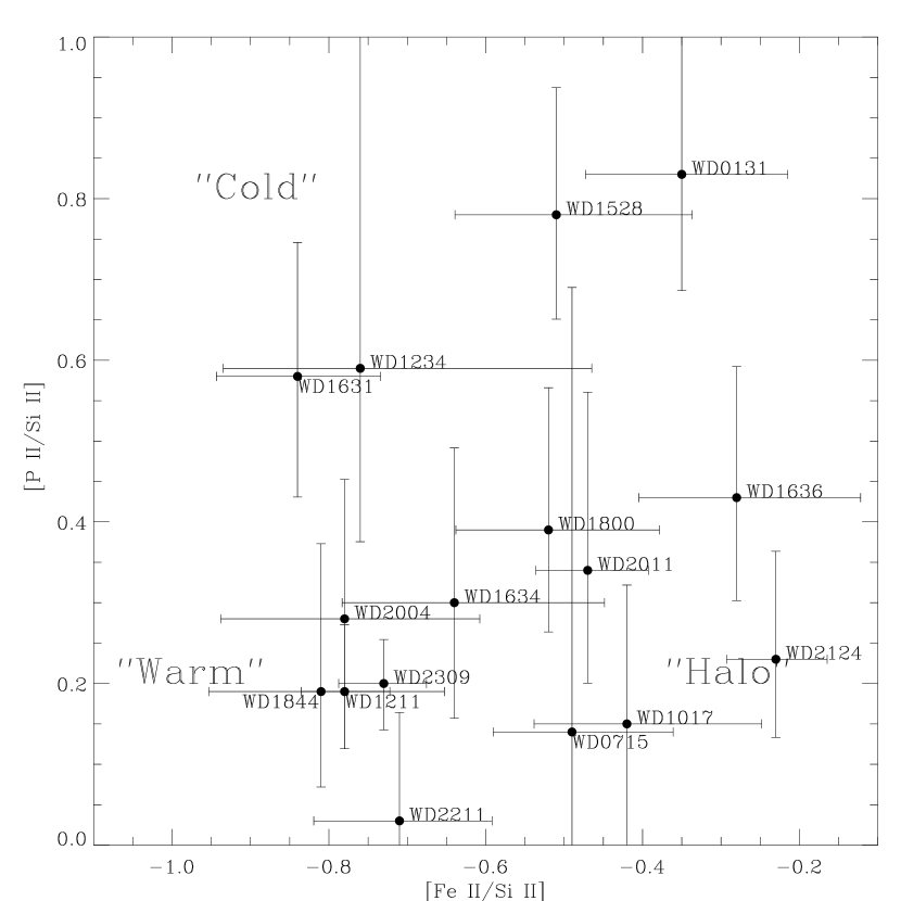
Plotting the results for [P II/Si II] and [Fe II/Si II] for common sightlines could a priori differentiate between the different depletion patterns since the cold, warm, and halo depletion patterns have different locii. Figure 8 shows [P II/Si II] versus [Fe II/Si II] along with the expected depletion patterns observed in more distant sightlines in the Galaxy. Most of the clouds appear to be dominated by more warm-like or halo-like gas than cold gas. The scatter is probably mainly explained by the fact that the clouds are not resolved and therefore are a combination of different gas phases. The sightline toward WD 0131163 is more complicated to understand because [P II/Si II] points toward a cold depletion pattern while [Fe II/Si II] toward an halo depletion pattern.
The solar ratios of Si/C, P/C, Fe/C are , respectively. Toward the few sightlines where a measurement of C II was possible, the ratios ([Si II/C II], [P II/C II], [Fe II/C II]) are: toward WD 0549+158, toward WD 1254+224, toward WD 1314+293, toward WD 1634573. The two first sightlines do not have any stringent limits. Toward WD 1314+293, these ratios are compatible with a cloud having a cold depletion pattern (in agreement with the ratios of P/Si and Fe/Si). These ratios for WD 1634573 point also to a cold depletion pattern ([P II/C II] is, however, far too small), but this is in contradiction with the results from P/Si and Fe/Si (see Figure 8), which might suggest that there is a lack of dust containing C toward this sightline.
The main reason for the deficiencies of Si and Fe are understood to be due to the incorporation of some of the Fe and Si into dust grains. The scatter in the values may reflect changes in the dust fraction or complications in the ionization fractions that are similar to those that we found for N, Ar, and O. The fact that we do not observe any trend with the distance or total column density of the sightline is probably mainly due to the fact that the clouds are not resolved.
8 Electron Density and Cooling Rate in the LISM
8.1 Electron Density
If collisions with electrons are the principal source of fine-structure excitation of C II in the LISM, then the familiar collisional equilibrium equation between C II and C II* (e.g., Gry & Jenkins, 2001) can be simplified to
| (1) |
when and K. This relation provides an estimate of the electron density when the space densities are replaced by column densities. The collisions with neutral hydrogen atoms should not be significant in the LISM. Indeed, according to Fig. 3 of Keenan et al. (1986), H I cm-3 alters the inferred electron density only when , but our calculations indicate that H I cm-3 in the LISM as long as cm-3 K (see Figure 6).
There is no evidence of C being depleted into dust in the LISM (see § 7). P is also known to be only lightly depleted. Moreover, in other regions of the Galaxy, C and P have similar depletions (Savage & Sembach, 1996a). Differences in ionization of C and P are probably not important (C III) is small with respect to C II); see § 6 and Figure 6), so that we can write C II*C IIC II*P II, where the solar ratio dex.
Under these assumptions and assuming a temperature of K observed in LIC, we can determine the electron density. This is shown in the bottom panel of Figure 9. The mean value is cm-3. Toward Capella situated at a distance of pc, Wood & Linsky (1997) determined –0.23 cm-3. We also plot in Figure 9 the expected electron density from our model versus the shielding of H I (see § 6). All the points fall above this line, suggesting that they are probably multiple regions where the shielding in each region is much less than the total column density of the sightline.
8.2 Cooling Rate
Because carbon has a high abundance, one of the most efficient way for cooling the diffuse gas is via the excitation of the C II by collisions with electrons and hydrogen atoms followed by the spontaneous emission at 157.7 when the levels decay to the ground state. It follows that the C II cooling rate in erg s-1 per H I atom can be written (e.g., Savage & Sembach, 1996b),
| (2) |
where H IO I (see § 4). In those conditions, the mean value in our sample is dex. Using P II as a proxy for the total H (H I+H II) and assuming no depletion, we have dex in our sample. If a depletion of to dex is assumed for P (Savage & Sembach, 1996a; Welty et al., 1999), both determinations are in good agreement. This result is in agreement with previous determinations derived in the diffuse gas in other parts of the Galaxy via different methods (Gry, Lequeux, & Boulanger, 1992; Bock et al., 1993; Savage & Sembach, 1996b; Boulanger et al., 1996). Toward Capella, using the H I and C II* column densities from Wood et al. (2002b), dex, but increases by about 0.3 dex when using O I as a proxy of H I.
In the top panel of Figure 9, we show the cooling rate against the total H I column density, showing a clear anti-correlation between these two quantities. This likely indicates that for low column density sightlines, a substantial amount of C II is associated with ionized gas, which is not taken into account in the normalization by the H) column density.
9 High Velocity Components
The sightlines toward WD 0455282, WD 1202608, and WD 1528487 each show a high velocity component separated by , , and , respectively, with respect to the lower velocity component. In the different tables, the high velocity component is designated by the letter “a” after the star name. Toward WD 0455282 and WD 1528487, high velocity components are clearly detected only in the C II absorption line for the elements considered here. For WD 0455282, there is also a clear detection of this component in the H I Lyman lines. For WD 1528487, there is only a hint in the Lyman lines. This rules out misidentification due to a stellar line. For these two stars, the presence of C II absorption features and the non-detection of neutral species, in particular the strong O I 1039 line, implies that these clouds are mostly ionized.
Toward WD 1202608, several species are detected (see Table 4), making the identification as a high-velocity component unquestionable. In contrast to the two other sightlines which have a very low column density with respect to their low velocity counterparts, this cloud has comparable column densities compared to the lower velocity components for Si II and Fe II. However, it has much smaller column densities for the neutral species, O I and N I, implying that this cloud is predominantly ionized. In addition, N I/(N II+N I, showing that at least 91% of N is in an ionized form. A similar comment applies for Ar I, even though the result remains more uncertain for this atom. Unfortunately, we have no information for C III and Fe III, because the former is blended with the local component (but the large lower limit – the largest in our sample – suggests a fair amount of C III), and Fe III is confused by the moving stellar lines from this binary system. The column density of O I suggests an H I column density of dex, while Si II gives a total H column density of dex (it is a lower limit because Si can be substantially depleted onto dust grains), implying an H II column density dex.
Holberg et al. (1995) and Kruk, Chayer, & Dupuis (2003) argue that the origin of the high velocity component toward WD 1202608 may be a remnant from the ejected common envelope of the binary, assuming it is a relatively young system. Gry & Jenkins (2001) also identified two negative high velocity components in the line of sight toward CMa at and from the main component. The fact that the velocity of these components is always negative would also point toward a circumstellar origin. However, it should be noted that the high velocity features appear in pairs of stars. WD 0455282 is in the same part of the sky as CMa, and WD 1202608 is in the same part of the sky as WD 1528487. This suggests that in each of these two cases, the sightlines could be passing through a single gas cloud. If so, the clouds are probably much closer than the stars and because of the high ionization are likely well within the LB. Although the argument is not definitive, it does weigh against the hypothesis of stellar ejecta. Finally, we note that this study does not show widespread high-velocity components along many sight lines. In particular, there is no evidence of globally expanding gas at positive velocities as might be expected for the case of a recent supernova explosion positioned near the Sun.
10 Summary and Concluding Remarks
We present a comprehensive survey of the LISM which includes the main species available in the far-uv wavelength range (C II, C II*, C III, N I, N II, O I, Ar I, Si II, P II, Fe II, Fe III, and H2). The spectral resolution () is not sufficient for detailed analysis of velocity structures. However, the number of species available permit a study of some of the fundamental characteristics of the local interstellar gas by comparing the relative column densities, the ionization structure, the molecular content, and the indirect indication of dust.
Our survey detected only very diffuse molecular clouds (). H2 was detected in only six out of 31 sightlines all within a single sector of the sky (see Figure 1). Thus it appears that H2 is not widely distributed in the LISM. The derived H2 -values for the 6 sightlines in our sample range from 2.8 to 5 , implying thermal temperatures less than 900–3000 K. This is different from the temperature of 7000 K usually observed in local interstellar clouds, implying different gas phases in the LISM. Combining our results with previous work on H2 in the LISM shows that the molecular phases are not uniform. Molecular hydrogen can exist in diffuse clouds, but in some regions the molecular fractions are similar to the atomic content.
The comparison of column densities of Si II, P II, Fe II provides information on the dust depletions of LISM. The relative abundances of these species vary from sightline to sightline, again suggesting different gas-phases in the LISM. These abundance ratios are better represented by typical warm or halo diffuse clouds observed in more distant sightlines in the Galaxy rather than a cold depletion pattern.
The cooling rate in the LISM, (in erg s-1 H I atom-1, where the H I column density was determined from the O I column density), can be derived directly from the C II* absorption lines and has a mean value of dex, very similar to previous determinations. Higher values are observed at lower H I column densities, indicating that for low column density sightlines, a substantial amount of the C II must come from ionized gas. The electron density can also be inferred from the C II* absorption lines. Using P II as a proxy of C II and assuming a temperature of 7000 K, the electron density in the LISM is cm-3, but larger than the values predicted by our model. This disagreement likely indicates that there are multiple regions along the sightlines where the H I shielding in each region is much less than the total H I column density of the sightline.
The comparison of column densities of N I and Ar I to O I provides information on the ionization structure of the LISM. The N I/O I ratio is systematically dex subsolar in the LB. Near or beyond the LB boundary, the picture is far more complicated, with a scatter of N I/O I between dex subsolar to dex supersolar (WD 1636+351). Using measured values and lower limits on the N II column densities, we show that the observed deficiencies are likely due to ionization and not abundance variations or dust depletions. For most sightlines, the Ar I/O I ratios also show deficiencies of Ar I in the LB by dex with respect to the solar value, but with a larger scatter than for N I, and this scatter increases beyond the LB ranging from a solar value to dex subsolar.
More highly ionized species such as C III and Fe III are also available to constrain the ionization structure. C III appears to be ubiquitous in the LISM for our sample, and C III/C II appears to vary from sightline to sightline. The C III/C II ratio is however generally small; C III is not a dominant ion in the LISM. Fe III remains more elusive and is often completely lost in the stellar profile. But our limits on Fe III/Fe II indicate that Fe II is the dominant ion in the LISM.
We modified the photoionization code used by Sofia & Jenkins (1998) and Jenkins et al. (2000). In particular, we adopted the new radiation field calculated by Slavin & Frisch (1998) and added the atomic parameters for C, P, Si, S, and Fe. The calculations were performed for a sequence of models where the thermal pressure was set to a value of cm-3 K. These calculations show that O I follows H I very well, while N I and Ar I become progressively more deficient as the shielding from H I becomes smaller. The other elements (C, P, Si, S, and Fe) remain primarily in the singly ionized state. The assumed pressure also seems to give a reasonable set of values for C III/C II. However, the values calculated for Fe III/Fe II appear to be too low, although we have only one measured value of Fe III/Fe II, the rest are upper limits. According to our model, the fraction of Fe III is heavily dependent on the effect of charge exchange with neutral hydrogen and is therefore not a reliable tracer of ionized gas.
Ar I, N I and H I have similar recombination coefficients, so if the LISM was highly ionized at an earlier epoch by a strong shock and is in the process of recombining, these elements would have roughly equal ionized fractions. Our study contradicts this proposition by indicating that photoionization is a major contribution. We note, however, that in a few cases, [N I/O I] is approximatively equal to [Ar I/O I], suggesting that the ionization fraction of N could be as large as that of Ar, which contradicts our model. This could indicate the radiation field might be harder in some directions. However, our model does not provide a clear explanation for this phenomenon with respect to the different observational constraints, and other factors are needed to explain this condition (e.g., non-equilibrium collisional ionization or overabundance of Ar possibly due to a supernova).
The variations observed in the ratios of Ar I/O I, N I/O I, N I/(N I+N II), and C III/C II indicate that the photoionization conditions are probably not uniform in the LB and in the LISM. Such changes in the photoionization conditions might be linked to the patchiness observed in the distribution O VI absorption (Oegerle et al., 2003). These variations, in turn, may depend on the strength and direction of the magnetic field at the cloud boundaries. Slavin & Frisch (2002) argued that evaporative interfaces at the boundaries of the clouds (O VI absorption being a tracer of such interfaces) could account for a large fraction of the observed ionization. Better observational constraints will come from higher spectral resolution of far-UV spectra, in which the individual clouds can be resolved.
Finally, we note that our results do not strongly contradict the X-ray data. Juda et al. (1991) compared the Be and B band fluxes in a number of different directions and found that the ratio of the two did not change with the overall intensity. From this nearly linear relationship between Be and B band fluxes, they concluded that interspersed neutral gas within the LB must have an average density less than 0.025 cm-3. Unfortunately, their sky coverage was limited and most of their viewpoints were not near any of our targets. An exception is WD 0501527, for which H I (Lemoine et al., 2002), and pc, which gives H I cm-3, below their limits. But only 30°away from one of the X-ray directions, toward WD 1631+781, the same calculation gives 0.1 cm-3. It would be interesting to see if toward denser lines of sight (e.g., WD 0004+330 gives H I cm-3), there is measurable X-ray absorption in the lowest energy band.
References
- Abgrall et al. (1993a) Abgrall, H., Roueff, E., Launay, F., Roncin, J. Y., & Subtil, J. L. 1993a, A&AS, 101, 273
- Abgrall et al. (1993b) Abgrall, H., Roueff, E., Launay, F., Roncin, J. Y., & Subtil, J. L. 1993b, A&AS, 101, 323
- Allende Prieto, Lambert, & Asplund (2001) Allende Prieto, C., Lambert, D. L., & Asplund, M. 2001, ApJ, 556, L63
- Anders & Grevesse (1989) Anders, E., & Grevesse, N., 1989, Geochim. Cosmochim. Acta, 53, 197
- Andersson et al. (2002) Andersson, B.-G., Idzi, R., Uomoto, A., Wannier, P. G., Chen, B., Jorgensen, A. M. 2002, AJ, 124, 2164
- André et al. (2003a) André, M., et al. 2003a, ApJ, in press
- André et al. (2003b) André, M., et al. 2003b, ApJ, in preparation
- Bannister et al. (2003) Bannister, N. P., Barstow, M. A., Holberg, J. B., & Bruhweiler, F. C. 2003, MNRAS, 341, 477
- Bock et al. (1993) Bock, J. J., et al. 1993, ApJ, 410, L115
- Boulanger et al. (1996) Boulanger, F., et al. 1996, ApJ, 312, 256
- Bowyer, Drake, & Vennes (2000) Bowyer, S., Drake, J. J., & Vennes, S. 2000, ARA&A, 38, 231
- Breitschwerdt & Schmutzler (1994) Breitschwerdt, D., & Schmutzler, T. 1994, Nature, 371, 774
- Bruhweiler & Kondo (1982) Bruhweiler, F. C., & Kondo, Y., 1982, ApJ, 259, 232
- Cartledge et al. (2001) Cartledge, S. I. B. and Meyer, D. M. and Lauroesch, J. T., & Sofia, U. J. 2001, ApJ, 562, 394
- Chayer, Fontaine, & Wesemael (1995) Chayer, P., Fontaine, G., & Wesemael, F. 1995, ApJS, 99, 189
- Chayer et al. (2000) Chayer, P., Kruk, J. W., Ake, T. B., Dupree, A. K., Malina, R. F., Siegmund, O. H. W., Sonneborn, G., & Ohl, R. G. 2000, ApJ, 538, L91
- Dame et al. (1987) Dame, T. M., et al. 1987, ApJ, 322, 706
- Dupree & Raymond (1983) Dupree, A. K., & Raymond, J. C. 1983, ApJ, 275, L71
- Dupuis et al. (1995) Dupuis, J., Vennes, S., Bowyer, S., Pradhan, A. K., & Thejll, P. 1995, ApJ, 455, 574
- Dupuis et al. (2003) Dupuis, J., et al. 2003, ApJ, in preparation
- Feldman et al. (2001) Feldman, P. D., Sahnow, D. J., Kruk, J. W., Murphy, E. M., & Moos, H. W. 2001, J. Geophys. Res., 106, 8119
- Ferlet (1999) Ferlet, R. 1999, A&A Rev., 9, 153
- Friedman et al. (2002) Friedman, S. D., et al. 2002, ApJS, 140, 37
- Frisch & York (1983) Frisch, P. C., York, D. G. 1983, ApJ, 271, L59
- Frisch & Slavin (1996) Frisch, P. C., Slavin, J. 1996, Space Science Rev., 78, 223
- Frisch et al. (1999) Frisch, P. C., et al. 1999, ApJ, 525, 492
- Génova et al. (1990) Génova, R., Molaro, P., Vladilo, G., & Beckman, J. E. 1990, ApJ, 355, 150
- Gry (1996) Gry, C. 1996, Space Sci. Rev., 78, 239
- Gry et al. (2002) Gry, C., Boulanger, F., Nehmé, C., Pineau des Forêts, Habart, E., & Falgarone, E. 2002, A&A, 391, 675
- Gry & Jenkins (2001) Gry, C., & Jenkins, E. B. 2001, A&A, 367, 617
- Gry, Lequeux, & Boulanger (1992) Gry, C., Lequeux, J., & Boulanger, F. 1992, A&A, 266, 457
- Hébrard et al. (2003) Hébrard, G., et al. 2003a, ApJ, 140, 103
- Hébrard et al. (2003) Hébrard, G., et al. 2003, ApJ, in press
- Hobbs, Blitz, & Magnani (1986) Hobbs, L. M., Blitz, L., & Magnani, L. 1986, ApJ,306, L109
- Hobbs et al. (1988) Hobbs, L. M., Blitz, L., Penrase, B. E., Magnani, L., & Welty, D. E. 1988, ApJ, 327, 356
- Holberg, Barstow, & Sion (1998) Holberg, J. B., Barstow, M. A., & Sion, E. M. 1998, ApJ, 119, 207
- Holberg et al. (1995) Holberg, J. B., Saffer, R. A., Tweedy, R. W., & Barstow, M. A. 1995, ApJ, 452, L133
- Holmgren et al. (1990) Holmgren, D. E., Brown, P. J. F., Dufton, P. L., & Keenan, F. P. 1990, ApJ, 364, 657
- Holweger (2001) Holweger, H. 2001. in Solar and Galactic composition, ed. Wimmer-Schweingruber (Berlin: Springer).
- Hoopes et al. (2003) Hoopes, C. G., Sembach, K. R., Hébrard, G., Moos, H. W., & Knauth, D. C. 2003, ApJ, 586, 1094
- Howk et al. (2000) Howk, J. C., Sembach, K. R., Roth, K. C., & Kruk, J. W. 2000, ApJ, 544, 867
- Jenkins (1986) Jenkins, E. B. 1986, ApJ, 304, 739
- Jenkins et al. (2000) Jenkins, E. B., et al. 2000, ApJ, 538, L81
- Juda et al. (1991) Juda, M., Bloch, J. J., Edwards, B. C., McCammon, D., Sanders, W. T., Snowden, S. L., & Zhang, J. 1991, ApJ, 367, 182.
- Keenan et al. (1986) Keenan, F. P., Lennon, D. J., Johnson, C. T., & Kingston, A. E. 1986, MNRAS, 220, 571
- Keenan et al. (1990) Keenan, F. P., Bates, B., Dufton, P. L., Holmgren, D. E., & Gilheany, S. 1990, ApJ, 348, 322
- Kruk, Chayer, & Dupuis (2003) Kruk, J. W., Chayer, P., & Dupuis, J. 2003, Proc. 13th European Workshop on White Dwarfs, ASP Conf. Series, R. Silvotti and D. DeMartino eds.
- Kruk et al. (2002) Kruk, J. W., et al. 2002, ApJS, 140, 19
- Lallement (1996) Lallement, R., 1998, Space Sci. Rev., 78, 361
- Lallement (1998) Lallement, R., 1998, Lecture Notes in Physics, 506, 19
- Lallement et al. (1995) Lallement, R., Ferlet, R., Lagrange, A. M., Lemoine, M., & Vidal-Madjar., V. 1995, A&A, 304, 461
- Lehner et al. (2002) Lehner, N., Gry, C., Sembach, K. R., Hébrard, G., Chayer, P., Moos, H. W., Howk, J. C., & Désert, J. M. 2002, ApJS, 140, 81
- Lemoine et al. (2002) Lemoine, M., et al. 2002, ApJS, 140, 67
- Linsky (1996) Linsky, J. L. 1996, Space Sci. Rev., 78, 157
- Linsky et al. (1993) Linsky, J. L., et al. 1993, ApJ, 402, 694
- Linsky et al. (2000) Linsky, J. L., Redfield, S., Wood, B. E., & Piskunov, N. 2000, ApJ, 528, 756
- Luhman (2001) Luhman, K. L. 2001, ApJ, 560, 287
- Lyu & Bruhweiler (1996) Lyu, C., & Bruhweiler, F. C. 1996, ApJ, 459, 216
- Magnani, Blitz, & Mundy (1985) Magnani, L., Blitz, L., & Mundy, L. 1985, ApJ, 295, 402
- McClintock et al. (1975) McClintock, W., Henry, R. C., Moos, H. W., & Linsky, J. L. 1975, ApJ, 202, 733
- Meyer, Cardelli, & Sofia (1997) Meyer, D. M., Cardelli, J. A., & Sofia, U. J. 1997, ApJ, 490, L103
- Meyer, Jura, & Cardelli (1998) Meyer, D. M., Jura, M., & Cardelli, J. A. 1998, ApJ, 493, 222
- Meyer (1989) Meyer, J.-P. 1989, in Cosmic Abundances of Matter, ed. C. J. Waddington, (New York: AIP), 245
- Moos et al. (2000) Moos, H. W., et al. 2000, ApJ, 538, L1
- Moos et al. (2002) Moos, H. W., et al. 2002, ApJS, 140, 3
- Morton (1991) Morton, D. C. 1991, ApJS, 77, 119
-
Oegerle et al. (2003)
Oegerle, W.R., Jenkins, E.B., Shelton, R., Bowen, D.V., &
Chayer, P., 2003, ApJ, submitted
- Oliveira et al. (2003) Oliveira, C., Hébrard, G., Howk, J. C., Kruk, J. W., Chayer, P., & Moos, H. W. 2003, ApJ, 587, 235
- Perryman et al. (1997) Perryman, M. A. C., et al. 1997, A&A., 323, L49
- Redfield & Linsky (2000) Redfield, S., & Linsky, J. L. 2000, ApJ, 534, 825
- Redfield et al. (2002) Redfield, S., Linsky, J. L., Ake, T. B., Ayres, T. R., Dupree, A. K., Robinson, R. D., Wood, B. E., & Young, P. R. 2002, ApJ, 581, 626
- Redfield & Linsky (2003) Redfield, S., & Linsky, J. L. 2003, ApJ, submitted
- Sahnow et al. (2000) Sahnow, D. J., et al. 2000, ApJ, 538, L7
- Savage et al. (1977) Savage, B. D., Bohlin, R. C., Drake J. F., & Budich, W. 1977, ApJ, 216, 291
- Savage & Sembach (1991) Savage, B. D., & Sembach, K. R. 1991, ApJ, 379, 245
- Savage & Sembach (1996a) Savage, B. D., & Sembach, K. R. 1996a, ARA&A, 34, 279
- Savage & Sembach (1996b) Savage, B. D., & Sembach, K. R. 1996b, ApJ, 470, 893
- Sembach & Savage (1992) Sembach, K. R., & Savage, B. D. 1992, ApJS, 83, 147
- Sfeir et al. (1999) Sfeir, D. M., Lallement, R., Crifo, F., & Welsh, B. Y. 1999, A&A, 346, 785
- Shull & van Steenberg (1982) Shull, J. M., & Van Steenberg, M 1982, ApJS, 48, 95
- Slavin (1989) Slavin, J. D. 1989, ApJ, 346, 718
- Slavin & Frisch (1998) Slavin, J. D., & Frisch, P. C. 1998, in the Local Bubble and Beyond, D. Breitschwerdt, M. J. Freyberg & J. Trumper (Eds.) (Springer: Berlin), p. 305
- Slavin & Frisch (2002) Slavin, J. D., & Frisch, P. C. 2002, ApJ, 565, 364
- Sofia & Jenkins (1998) Sofia, U. J., & Jenkins, E. B. 1998, ApJ, 499, 951
- Sofia & Meyer (2001) Sofia, U. J., & Meyer, D. M. 2001, ApJ, 554, L221
- Sonneborn et al. (2002) Sonneborn, G., et al. 2002, ApJS, 140, 51
- Spitzer, Cochran, & Hirshfeld (1974) Spitzer, L., Cochran, W. D., & Hirshfeld, A. 1974, ApJS, 28, 373
- Spitzer et al. (1973) Spitzer, L., Drake, J. F., Jenkins, E. B., Morton, D. C., Rogerson, J. B., & York, D. G. 1973, ApJS, 181, L116
- Tat & Terzian (1999) Tat, H. H., & Terzian, Y. 1999, PASP, 111, 1258
- Trapero et al. (1996) Trapero, J., Sempere, M. J., Beckman, J. E., Hobbs, L. M. 1996, ApJ, 457, 731
- Vallerga (1998) Vallerga, J. V. 1998, ApJ, 497, 921
- Vallerga et al. (1993) Vallerga, J. V., Vedder, P. W., Craig, N., & Welsh, B. Y. 1993, ApJ, 411, 729
- Vennes et al. (1998) Vennes, S., Dupuis, J., Chayer, P., Polomski, E. F., Dixon, W. V. D, & Hurwitz, M. 1998, ApJ, 500, L41
- Vennes et al. (1997) Vennes, S., Thejll, P. A., Galvan, R. G., & Dupuis, J. 1997, ApJ, 480, 714
- Vidal-Madjar et al. (1998) Vidal-Madjar, A., et al. 1998 A&A, 338, 694
- Welsh et al. (1999) Welsh, B. Y,; Sfeir, D. M., Sirk, M. M., & Lallement, R. 1999, A&A, 353, 308
- Welty et al. (1999) Welty, D. E., Hobbs, L. M., Lauroesch, J. T., Morton, D. C., Spitzer, L., & York, D. G. 1999, ApJS, 124, 465
- Wiese, Bonvallet, & Lawler (2002) Wiese, L. M., Bonvallet, G. A., & Lawler, J. E. 2002, ApJ, 569, 1032
- Wolff, Koester, & Lallement (1999) Wolff, B., Koester, D., & Lallement, R. 1999, A&A, 329, 1045
- Wood & Linsky (1997) Wood, B. E., & Linsky, J. L. 1997, ApJ, 474, L39
- Wood et al. (2002a) Wood, B. E., et al. 2002a, ApJS, 140, 91
- Wood et al. (2002b) Wood, B. E., Redfield, S., Linsky, J. L., & Sahu, M. S. 2002b, ApJ, 581, 1168
| WD name | Other name | Spectral | Aperture | Notes | ||||
|---|---|---|---|---|---|---|---|---|
| (°) | (°) | () | (pc) | Type | ||||
| WD 0004330 | GD 2 | 112.48 | 97a | DA | LWRS, MDRS | [A] (1) | ||
| WD 0050332 | GD 659 | 299.15 | 58a | DA1 | LWRS | [B] (2) | ||
| WD 0131163 | GD 984 | 167.26 | 96a | DA1 | LWRS | [B] (2) | ||
| WD 0455282 | MCT 0455-2812 | 229.29 | 102a | DA1 | MDRS | [C] (2) | ||
| WD 0501527 | G191-B2B | 155.95 | (59a) | DA1 | LWRS, MDRS, HIRS | [C] (3) | ||
| WD 0549158 | GD 71 | 192.03 | 49a | DA1 | LWRS | [A] (2) | ||
| WD 0621376 | 245.41 | 78a | DA | LWRS, MDRS | [D] (4) | |||
| WD 0715703 | 281.62 | 94a | DA1 | MDRS | [A] (2) | |||
| WD 1017138 | 255.74 | 90a | DA | LWRS | [A] (2) | |||
| WD 1202608 | GD 314, Feige 55 | 133.11 | 200d | DA | MDRS | [C] (2) | ||
| WD 1211332 | HZ 21 | 175.03 | DO | LWRS, MDRS | [B] (5) | |||
| WD 1234481 | 129.81 | 129a | DA | LWRS | [A] (2) | |||
| WD 1254223 | GD 153 | 317.26 | 67a | DA1 | LWRS | [A] (2) | ||
| WD 1314293 | HZ 43 | 54.10 | DA1 | LWRS, MDRS | [A] (6) | |||
| WD 1528487 | 78.87 | 140a | DA: | LWRS | [B] (2) | |||
| WD 1615154 | EGGR 118 | 358.79 | 55d | DA1.5 | MDRS | [A] (2) | ||
| WD 1631781 | 1ES 1631+78.1 | 111.29 | 67a | DA1 | MDRS | [A] (7) | ||
| WD 1634573 | HD 149499 B | 329.88 | α | DOZ1 | LWRS, MDRS | [B] (8) | ||
| WD 1636351 | 56.98 | 109a | DA | LWRS | [A] (2) | |||
| WD 1800685 | 98.73 | 159a | DA1 | MDRS | [A] (2) | |||
| WD 1844223 | 12.50 | 62a | DA: | LWRS | [A] (2) | |||
| WD 2004605 | 336.58 | 58a | DA | MDRS | [A] (7) | |||
| WD 2011395 | EUVE J2013+40.0 | 77.00 | 141a | DAO | LWRS | [B] (2) | ||
| WD 2111498 | GD 394 | 91.37 | 50a | DA2 | LWRS | [B] (2) | ||
| WD 2124224 | 26.81 | 224b | DA | MDRS | [B] (2) | |||
| WD 2148286∗ | BD+28°4211 | 81.87 | β | SdO | LWRS, MDRS | [E] (9) | ||
| WD 2152548 | 339.73 | 128a | DA: | MDRS | [A] (2) | |||
| WD 2211495 | 345.79 | 53a | DA | LWRS, MDRS, HIRS | [D] (10) | |||
| WD 2247583 | Lan 23 | 107.64 | 122a | DA | lWRS | [C] (5) | ||
| WD 2309105 | GD 246 | 87.26 | 79a | DA1 | LWRS, MDRS | [B] (5) | ||
| WD 2331475 | MCT 2331-4731 | 334.83 | 82a | DA | lWRS, MDRS | [B] (5) |
Note. — Heliocentric velocities are from Holberg, Barstow, & Sion (1998), except () from Wood et al. (2002a) and () from Sonneborn et al. (2002). ∗Note that using the denomination WD 2148286 for BD+28°4211 is somewhat incorrect because this star is a subdwarf of type O, not a white dwarf. However, for consistency and simplicity, we have used this name throughout the article. : Distances from Vennes et al. (1997). : Distance from Vennes et al. (1998). : Distance from Dupuis (2002, private communication). : Distances from Holberg, Barstow, & Sion (1998). Distances with errors are from Hipparcos parallax measurements (Perryman et al., 1997); for the others, the errors are typically 20–30%. Metallicity of the star: [A] no metal detected in FUSE spectra; [B] few metals; [C] rich in metals; [D] very rich in metals; [E] solar metallicity (see Dupuis et al. 2003, in preparation, and references below). Source of the column densities: (1) Oliveira et al. (2003, private communication), this work; (2) this work; (3) Lemoine et al. (2002); André et al. (2003b); (4) Lehner et al. (2002), this work; (5) Oliveira et al. (2003), this work; (6) Kruk et al. (2002); (7) Hébrard et al. (2003), this work; (8) Wood et al. (2002a), this work; (9) Sonneborn et al. (2002), this work; (10) Hébrard et al. (2003), this work.
| Ions | Note | ||
|---|---|---|---|
| (Å) | |||
| C II | 1036.337 | saturated () | |
| C II* | 1037.018 | ||
| C III | 977.020 | blended () | |
| N I | 952.303 | ||
| 952.415 | |||
| 953.415 | |||
| 953.655 | |||
| 953.970 | |||
| 963.990 | |||
| 964.626 | |||
| 965.041 | |||
| 1134.165 | airglow () | ||
| 1134.415 | airglow () | ||
| 1134.980 | airglow () | ||
| N II | 1083.994 | saturated () | |
| O I | 919.658 | ||
| 919.917 | |||
| 921.857 | |||
| 922.200 | |||
| 924.950 | |||
| 925.446 | |||
| 929.517 | |||
| 930.257 | |||
| 936.630 | |||
| 948.686 | |||
| 950.885 | |||
| 976.448 | |||
| 1039.230 | airglow () | ||
| Si II | 1020.699 | ||
| Ar I | 1048.220 | ||
| 1066.660 | blended () | ||
| P II | 1152.818 | ||
| Fe II | 1055.262 | ||
| 1063.176 | |||
| 1096.877 | |||
| 1125.448 | |||
| 1143.226 | |||
| 1144.938 | |||
| Fe III | 1122.524 |
Note. — Rest frame vacuum wavelengths and oscillator strengths are from Morton (private communication, 2000), except for the -values of Fe II which are from Howk et al. (2000). () These lines are generally strong and usually only a lower limit can be estimated (except in few cases where the column densities are extremely small). () Interstellar C III can be blended with the stellar component if the star contains some metals. () Those lines can be affected by airglow emission lines, especially the N I triplet. () Ar I 1066 can be blended with stellar Si IV 1066 if the star contains some metals.
| Sightline | [O I] | [N I] |
|---|---|---|
| () | () | |
| WD 0004330 | ||
| WD 0050332 | ||
| WD 0131163 | ||
| WD 0455282 | ||
| WD 0715703 | ||
| WD 1017138 | ||
| WD 1202608 | ||
| WD 1234481 | ||
| WD 1528487 | ||
| WD 1615154 | ||
| WD 1631781 | ||
| WD 1636351 | ||
| WD 1800685 | ||
| WD 1844223 | ||
| WD 2004605 | ||
| WD 2111498 | ||
| WD 2124224 | ||
| WD 2152548 | ||
| WD 2331475 |
Note. — “” means that the -value was taken from the other species; see text.
| Star | C II | C II* | C III | O I | N I | N II | Si II | Ar I | Fe II | Fe III | P II |
|---|---|---|---|---|---|---|---|---|---|---|---|
| 16.20 | 15.15 | 13.55 | 12.83 | ||||||||
| WD 0004330 | 14.38 | 13.51 | 13.40 | 16.35 | 15.30 | 14.12 | 14.34 | 13.80 | 13.60 | 12.95 | 12.85 |
| 16.50 | 15.45 | 13.68 | 12.87 | ||||||||
| 12.29 | 15.21 | 14.01 | 12.80 | ||||||||
| WD 0050332 | 14.09 | 12.55 | 13.14 | 15.26 | 14.30 | 13.91 | 13.60 | 12.67 | 13.06 | 12.39 | |
| 12.71 | 15.32 | 14.60 | 13.22 | ||||||||
| 12.84 | 15.83 | 14.80 | 13.80 | 12.90 | 13.51 | 12.66 | |||||
| WD 0131163 | 14.20 | 13.00 | 13.27 | 15.89 | 14.91 | 14.11 | 13.93 | 12.97 | 13.54 | 12.78 | |
| 13.12 | 15.97 | 15.04 | 14.05 | 13.03 | 13.57 | 12.87 | |||||
| 13.54 | |||||||||||
| WD 0455282a | 13.58 | 12.68 | 12.66 | 14.12 | 13.13 | 13.47 | 12.88 | 12.62 | 12.73 | 12.39 | |
| 13.62 | |||||||||||
| 12.46 | 13.29 | 12.83 | |||||||||
| WD 0455282b | 14.20 | 12.68 | 13.72 | 14.91: | 13.44 | 13.92 | 13.34: | 12.62 | 12.94 | 12.99 | 12.39 |
| 12.83 | 13.59 | 13.02 | |||||||||
| 13.23 | 14.82 | 13.83 | 13.51 | 13.03 | |||||||
| WD 0501527 | 15.39 | 13.26 | 14.86 | 13.87 | 13.83 | 13.52 | 12.00 | 13.05 | 11.85 | ||
| 13.28 | 14.90 | 13.91 | 13.53 | 13.07 | |||||||
| 13.79 | 12.59 | 14.18 | 13.43 | 12.75 | |||||||
| WD 0549158 | 13.81 | 12.84 | 12.72 | 14.27 | 13.60 | 13.49 | 12.99 | 12.46 | 12.64 | 13.12 | 12.23 |
| 13.84 | 12.81 | 14.34 | 13.54 | 13.14 | |||||||
| 13.04 | 15.22 | 14.27 | 12.79 | 12.79 | |||||||
| WD 0621376 | 14.19 | 13.09 | 13.31 | 15.26 | 14.34 | 13.80 | 13.68 | 12.86 | 12.94 | ||
| 13.14 | 15.31 | 14.41 | 12.93 | 13.05 | |||||||
| 13.31 | 15.81 | 14.89 | 13.97 | 13.09 | 13.52 | 11.76 | |||||
| WD 0715703 | 14.29 | 13.42 | 13.22 | 15.90 | 14.96 | 14.00 | 14.09 | 13.17 | 13.56 | 13.34 | 12.25 |
| 13.51 | 16.00 | 15.04 | 14.18 | 13.25 | 13.61 | 12.47 | |||||
| 12.93 | 13.05 | 15.73 | 14.46 | 13.90 | 13.02 | 13.55 | 12.18 | ||||
| WD 1017138 | 14.10 | 13.10 | 13.14 | 15.95 | 14.55 | 13.90 | 14.06 | 13.17 | 13.60 | 12.23 | |
| 13.23 | 13.21 | 16.40 | 14.64 | 14.17 | 13.28 | 13.65 | 12.57 | ||||
| 12.28 | 14.57 | 13.12 | 14.05 | 11.88 | 13.68 | ||||||
| WD 1202608a | 14.83 | 12.60 | 14.14 | 14.70 | 13.37 | 14.38 | 14.11 | 12.18 | 13.72 | ||
| 12.78 | 14.84 | 13.42 | 14.17 | 12.55 | 13.77 | ||||||
| 12.94 | 15.63 | 14.75 | 14.13 | 12.90 | 13.70 | ||||||
| WD 1202608b | 14.65 | 13.07 | 14.14 | 15.65 | 14.77 | 14.10 | 14.19 | 13.07 | 13.74 | ||
| 13.17 | 15.68 | 14.79 | 14.25 | 13.19 | 13.78 | ||||||
| 13.07 | 15.69 | 14.73 | 14.32 | 13.13 | 13.50 | 12.50 | |||||
| WD 1211332 | 14.39 | 13.14 | 13.49 | 15.74 | 14.77 | 14.03 | 14.36 | 13.16 | 13.54 | 13.43 | 12.57 |
| 13.19 | 15.79 | 14.81 | 14.40 | 13.19 | 13.58 | 12.63 | |||||
| 12.74 | 15.56 | 14.58 | 13.65 | 12.83 | 12.92 | 12.14 | |||||
| WD 1234481 | 14.23 | 12.89 | 13.60 | 15.63 | 14.62 | 14.15 | 13.87 | 12.90 | 13.07 | 12.48 | |
| 13.01 | 15.71 | 14.67 | 14.01 | 12.96 | 13.19 | 12.66 | |||||
| 13.62 | 14.26 | 13.25 | 12.96 | 11.71 | |||||||
| WD 1254223 | 13.64 | 12.66 | 12.20: | 14.38 | 13.30 | 13.07 | 12.69 | 12.04 | 12.54 | 12.94 | 12.30 |
| 13.66 | 14.58 | 13.45 | 13.16 | 12.23 | |||||||
| 14.66 | 12.54 | 14.48 | 13.48 | 13.54 | 12.74 | 11.71 | 12.15 | ||||
| WD 1314293 | 14.83 | 12.73 | 12.59 | 14.51 | 13.51 | 13.62 | 12.85 | 11.96 | 12.17 | 12.64 | 11.97 |
| 14.92 | 12.64 | 14.54 | 13.54 | 13.69 | 12.94 | 12.11 | 12.19 | ||||
| 13.26 | |||||||||||
| WD 1528487a | 13.32 | 12.88 | 13.55: | 14.07 | 13.46 | 13.22 | 13.04 | 12.55 | 13.22 | 13.30 | 12.56 |
| 13.36 | |||||||||||
| 12.89 | 15.72 | 14.95 | 13.80 | 13.42 | 13.24 | 12.10 | |||||
| WD 1528487b | 14.23 | 12.99 | 13.55: | 15.80 | 14.99 | 14.03 | 13.91 | 13.46 | 13.36 | 13.30 | 12.40 |
| 13.05 | 15.88 | 15.04 | 14.01 | 13.49 | 13.45 | 12.70 | |||||
| 13.08 | 12.78 | 15.68 | 14.93 | 13.61 | 13.27 | 13.44 | 12.39 | ||||
| WD 1615154 | 14.03 | 13.17 | 12.96 | 15.78 | 15.03 | 13.71 | 13.94 | 13.29 | 13.50 | 13.16 | 12.45 |
| 13.25 | 13.09 | 15.89 | 15.18 | 13.79 | 13.31 | 13.57 | 12.59 | ||||
| 13.02 | 15.81 | 15.18 | 14.01 | 13.45 | 13.20 | 12.59 | |||||
| WD 1631781 | 14.32 | 13.17 | 13.41 | 15.90 | 15.28 | 14.12 | 14.11 | 13.53 | 13.23 | 12.68 | 12.71 |
| 13.32 | 15.99 | 15.38 | 14.21 | 13.61 | 13.26 | 12.83 | |||||
| 15.65 | 15.48 | 14.58 | 14.72 | 13.59 | 13.20 | 13.01 | 12.01 | ||||
| WD 1634573 | 15.90 | 15.4 | 15.51 | 14.62 | 14.90 | 13.76 | 13.26 | 13.08 | 12.08 | ||
| 16.25 | 15.54 | 14.66 | 15.08 | 13.89 | 13.32 | 13.15 | 12.15 | ||||
| 13.23 | 15.58 | 14.15 | 13.64 | 13.94 | 12.70 | ||||||
| WD 1636351 | 14.25 | 13.34 | 13.27 | 15.71 | 15.08 | 14.08 | 14.30 | 13.70 | 13.98 | 13.41 | 12.75 |
| 13.44 | 15.95 | 14.42 | 13.76 | 14.02 | 12.80 | ||||||
| 13.57 | 16.02 | 15.02 | 14.44 | 13.81 | 13.87 | 12.14 | 12.80 | ||||
| WD 1800685 | 14.47 | 13.63 | 13.56 | 16.12 | 15.05 | 14.21 | 14.53 | 13.83 | 13.97 | 12.80 | 12.94 |
| 13.67 | 16.26 | 15.09 | 14.60 | 13.93 | 14.07 | 13.05 | 13.05 | ||||
| 12.87 | 15.85 | 14.91 | 14.28 | 13.54 | 13.42 | 12.45 | |||||
| WD 1844223 | 14.16 | 13.04 | 13.25 | 15.97 | 15.06 | 13.82 | 14.38 | 13.58 | 13.53 | 13.11 | 12.59 |
| 13.16 | 16.15 | 15.36 | 14.45 | 13.62 | 13.66 | 12.69 | |||||
| 12.81 | 13.12 | 15.57 | 14.76 | 13.92 | 13.18 | 13.18 | 12.30 | ||||
| WD 2004605 | 14.02 | 12.99 | 13.15 | 15.65 | 14.84 | 13.85 | 14.07 | 13.26 | 13.25 | 12.90 | 12.37 |
| 13.17 | 13.17 | 15.73 | 14.92 | 14.22 | 13.34 | 13.32 | 12.44 | ||||
| 13.35 | 16.01 | 15.20 | 14.16 | 13.40 | 13.69 | 12.39 | |||||
| WD 2011395 | 14.39 | 13.38 | 13.48 | 16.06 | 15.48 | 14.34 | 14.23 | 13.43 | 13.72 | 14.09 | 12.59 |
| 13.41 | 16.12 | 15.61 | 14.29 | 13.93 | 13.75 | 12.72 | |||||
| 13.05 | 15.00 | 13.97 | 13.31 | 12.46 | 13.29 | ||||||
| WD 2111498 | 14.12 | 13.12 | 13.00 | 15.06 | 14.00 | 13.91 | 13.35 | 12.58 | 13.23 | 12.47 | |
| 13.18 | 15.11 | 14.08 | 13.31 | 12.68 | 13.35 | ||||||
| 13.41 | 15.91 | 14.93 | 14.44 | 13.50 | 14.18 | 12.62 | |||||
| WD 2124224 | 14.57 | 13.47 | 13.75 | 15.94 | 14.97 | 14.32 | 14.49 | 13.57 | 14.22 | 12.74 | |
| 13.52 | 15.97 | 15.04 | 14.53 | 13.64 | 14.27 | 12.83 | |||||
| 13.73 | 16.17 | 15.48 | |||||||||
| WD 2148286 | 14.43 | 13.75 | 13.54 | 16.22 | 15.55 | 14.13 | 13.60 | ||||
| 13.76 | 16.27 | 15.62 | |||||||||
| 12.65 | 15.42 | 14.37 | 13.38 | 12.56 | 13.34 | ||||||
| WD 2152548 | 14.30 | 12.95 | 13.37 | 15.49 | 14.42 | 14.12 | 13.76 | 12.72 | 13.37 | 13.23 | 12.84 |
| 13.13 | 15.59 | 14.48 | 13.97 | 12.90 | 13.40 | ||||||
| 12.79 | 15.31 | 14.27 | 14.45 | 13.92 | 12.77 | 13.17 | 11.95 | ||||
| WD 2211495 | 14.34 | 12.88 | 13.58 | 15.34 | 14.30 | 14.60 | 14.00 | 12.82 | 13.25 | 12.05 | |
| 12.96 | 15.38 | 14.33 | 14.75 | 14.08 | 12.87 | 13.33 | 12.15 | ||||
| 13.56 | 16.53 | 15.66 | 13.96 | ||||||||
| WD 2247583 | 14.41 | 13.59 | 13.31 | 16.72 | 15.73 | 13.95 | 14.03 | 13.14 | |||
| 13.63 | 16.87 | 15.80 | 14.10 | ||||||||
| 13.05 | 15.63 | 14.72 | 14.05 | 13.09 | 13.25 | 12.24 | |||||
| WD 2309105 | 14.20 | 13.08 | 13.37 | 15.67 | 14.75 | 13.81 | 14.07 | 13.14 | 13.30 | 12.29 | |
| 13.10 | 15.71 | 14.78 | 14.10 | 13.21 | 13.35 | 12.34 | |||||
| 13.18 | 15.42 | 14.48 | 13.89 | 12.67 | 13.27 | 12.08 | |||||
| WD 2331475 | 14.43 | 13.27 | 13.60 | 15.48 | 14.53 | 14.27 | 13.99 | 12.77 | 13.32 | 12.18 | |
| 13.36 | 15.54 | 14.58 | 14.09 | 13.87 | 13.37 | 12.28 |
Note. — For a given sightline and a given species, there are 3 entries: the second number corresponds to the most likely value, while the first and third correspond to and , respectively. indicates a 3 upper limit detection, except in the case of C III where the upper limit reflects that this line may be blended with the C III photospheric lines. indicates a lower limit, i.e. the line is saturated. Colon means that the value is uncertain. See § 3 and Table 1 for more details and references, respectively. Two entries for one sightline (denoted by a and b) indicate that two components are detected with FUSE: for WD 0455282, component a is at and b at ; for WD 1202608, component a is at and b at ; and for WD 1528487, component a is at and b at .
| Sightline | |||||||
|---|---|---|---|---|---|---|---|
| () | (K) | ||||||
| WD 0004330 | (1) | (22) | (10) | (4) | 14.46 | a | |
| WD 1636351 | (7) | (25) | (13) | (3) | 15.05 | ||
| WD 1800685 | (5) | (12) | (12) | (1) | 14.75 | ||
| WD 2011395 | (13) | (2) | (2) | 14.22 | |||
| WD 2148286 | (4) | (8) | (13) | (14) | 15.38 | ||
| WD 2247583 | (6) | (13) | (14) | (7) | 15.11 |
Note. — The number of lines used to measure the column density is shown in parentheses. For WD 0004330, WD 2148286, and WD 2247583, the column densities and -values are from Oliveira et al. (2003, private communication) Sonneborn et al. (2003, erratum in preparation), and Oliveira et al. (2003), respectively. For WD 0004330, only the -levels could be fitted in the temperature relation within 1 error bar, K.
| Sightlines | [Ar I/O I] | [N I/O I] | N I/(N II+N I) |
|---|---|---|---|
| WD 0004330 | |||
| WD 0050332 | |||
| WD 0131163 | |||
| WD 0455282b | |||
| WD 0501527 | |||
| WD 0549158 | |||
| WD 0621376 | |||
| WD 0715703 | |||
| WD 1017138 | |||
| WD 1202608a | |||
| WD 1202608b | |||
| WD 1211332 | |||
| WD 1234481 | |||
| WD 1254223 | |||
| WD 1314293 | |||
| WD 1528487b | |||
| WD 1615154 | |||
| WD 1631781 | |||
| WD 1634573 | |||
| WD 1636351 | |||
| WD 1800685 | |||
| WD 1844223 | |||
| WD 2004605 | |||
| WD 2011395 | |||
| WD 2111498 | |||
| WD 2124224 | |||
| WD 2148286 | |||
| WD 2152548 | |||
| WD 2211495 | |||
| WD 2247583 | |||
| WD 2309105 | |||
| WD 2331475 |
Note. — Suffix “a” after star names means it is a high velocity component (see § 9), while “b” means that it is the low velocity component. Colon means that the value is uncertain.
| Targets | C IIIC II)] | C IIIC II)]c | Note |
|---|---|---|---|
| WD 0050332 | to | C II LL, C III SC? | |
| WD 0131163 | C II LL | ||
| WD 0455282a | C III UL | ||
| WD 0549158 | to | C III SC? | |
| WD 0621376 | C II LL, C III SC | ||
| WD 1017138 | C II LL | ||
| WD 1254223 | C III SC? | ||
| WD 1314293 | to | C III SC? | |
| WD 1528487a | C III LL | ||
| WD 1615154 | C II LL | ||
| WD 1634573 | C III SC | ||
| WD 2004605 | C II LL | ||
| WD 2011395 | C II LL, C III SC | ||
| WD 2111498 | C II LL, C III SC |
Note. — The second column presents the raw measurement, while the third one includes possible stellar correction for C III. When two numbers are indicated in the third column, it means that only an upper limit was derived for the amount of photospheric C III 977. LL: lower limit. UL: upper limit. SC: C III stellar contamination. SC?: possible C III stellar contamination. Suffix “a” after star names means the ratio is for a high velocity component (see § 9), and this component is not blended with any stellar lines. Colon means that the value is uncertain.
| Targets | Fe IIIFe II)] |
|---|---|
| WD 0004330 | |
| WD 0455282b | |
| WD 0715703 | |
| WD 1211332 | |
| WD 1314293 | |
| WD 1528487b | |
| WD 1615154 | |
| WD 1631781 | |
| WD 1636351 | |
| WD 1800685 | |
| WD 1844223 | |
| WD 2004605 | |
| WD 2011395 | |
| WD 2152548 | |
| WD 2247583 |
Note. — Here “” is a 3 upper limit. Colon means that the value is uncertain.