Gauge Coupling Variation in Brane Models

Abstract

We consider the space-time variation of gauge couplings in brane-world models induced by the coupling to a bulk scalar field. A variation is generated by the running of the gauge couplings with energy and a conformal anomaly while going from the Jordan to the Einstein frame. We indicate that the one-loop corrections cancel implying that one obtains a variation of the fine structure constant by either directly coupling the gauge fields to the bulk scalar field or having bulk scalar field dependent Yukawa couplings. Taking into account the cosmological dynamics of the bulk scalar field, we constrain the strength of the gauge coupling dependence on the bulk scalar field and relate it to modifications of gravity at low energy.

Physics beyond the standard model predicts the existence of scalar degrees of freedom, moduli fields, whose presence modify general relativity even at low energy. Within the framework of brane-world models these moduli fields are directly associated with the possible deformations of the bulk-brane configurations, i.e. the free motion of branes relative to each other (see e.g. braxvdbruckreview for recent reviews on brane worlds). The presence of such massless fields is generally thought to lead to large deviations with respect to general relativity, prompting the need for a stabilization of the moduli. Within string theory this is the case for the dilaton field whose expectation value is related to the gauge coupling constant at the unification scale. Such a running dilaton is ruled out experimentally. Attempts to stabilize the dilaton have been notoriously difficult to justify and require ingredients such as non-perturbative effects and supersymmetry breaking.

The time evolution of the moduli fields does not only imply modifications to general relativity but may also provide a hint towards extensions to the standard model sector. Phenomena such as the variation of coupling constants may spring from the fact that these couplings are effective parameters depending on the moduli. In this paper we will discuss the time-variation of coupling parameters in brane models. (See e.g. Calmet & Fritzsch –Kostelecky for recent discussions on varying constants. Reference uzan is a recent discussion on experimental and theoretical aspects of varying constants and has an extensive list of literature.)

We restrict the present analysis to the case in which the gauge couplings depend on the evolution of a single scalar field $\psi$. Let us consider the gauge couplings $\alpha_{i}=g_{i}^{2}/4\pi$ to one loop order

$$\alpha_{i}^{-1}(E,\psi)=\alpha_{i}^{-1}(\tilde{E},\psi)+\frac{b_{i}}{2\pi}\ln(\tilde{E}/E),$$ (1)

where $E$ and $\tilde{E}$ are two arbitrary energy scales, and $b_{i}$ are the renormalization group equation coefficients. Notice that the renormalization group coefficients are pure numbers determined solely by the matter content of the model. These coefficients may be taken as the standard model ones, $b^{SM}_{i}=(41/10,-19/6,-7)$. We have emphasized the explicit dependence on the scalar field $\psi$. In this way, a variation of the couplings $\alpha_{i}$ over cosmological meaningful periods would be a consequence of the evolution of $\psi$.

In the Einstein frame where the Planck mass is time-independent, the physical masses $M$ may depend on the scalar field $\psi$. If this is the case, the total variation of the gauge coupling involves the variation of $M$. From relation (1), this total variation reads

$$\delta\alpha_{i}^{-1}(M,\psi)=\delta_{\psi}\alpha_{i}^{-1}(m_{\rm Pl},\psi)-\frac{b_{i}}{2\pi}\frac{\delta_{\psi}M}{M},$$ (2)

where $M$ is the energy scale at which one measures the gauge coupling. One can be more specific in a large class of theories where the effective four dimensional action has the generic form

$$S_{\rm J}\supset\int d^{4}x\sqrt{-g}\left[\frac{A^{-2}{\cal R}}{{2\kappa^{2}_{4}}}-\frac{1}{4g_{J}^{2}}F^{2}\right],$$ (3)

in the Jordan frame where matter couples to $g_{\mu\nu}$, as opposed to the Einstein frame, where Newton’s constant is moduli field-independent. In the above expression $A$ depends on the scalar field $\psi$, $F$ is the antisymmetric gauge tensor field, and $g_{J}$ is the gauge coupling in the Jordan frame (which could have a dependence on the moduli field). To go to the Einstein frame formulation we must perform the conformal transformation

$$g_{\mu\nu}\rightarrow A^{-2}g_{\mu\nu}.$$ (4)

The masses of particles are affected according to US

$$M_{E}=AM_{J},$$ (5)

while the bare dimensionless coupling constants remain unaffected, $g_{J}\rightarrow g_{E}=g_{J}$. This picture is modified quantum mechanically Fujii Maeda . In the Einstein frame, the relation between the bare and the renormalized couplings, $g_{B}$ and $g$, using dimensional regularization is

$$g_{B}=\mu^{2-d/2}g\left[1+g^{2}\frac{b}{32\pi^{2}}\Gamma(2-d/2)\right],$$ (6)

where $\mu$ is the renormalization group energy scale. The dependence between the bare coupling $g_{B}$ in the Einstein frame and the bare coupling $g_{J}$ in the Jordan frame is $g_{B}=A^{2-d/2}g_{J}$. Then, it follows

$$g_{J}=(\mu/A)^{2-d/2}g\left[1+g^{2}\frac{b}{32\pi^{2}}\Gamma(2-d/2)\right].$$ (7)

We consider its direct dependence on the scalar field $\psi$ by introducing a function $D(\psi)$ in such a way that

$$4\pi\,\delta_{\psi}(g_{J}^{-2})=\delta_{\psi}D(\psi).$$ (8)

Now, taking into account the dependence of both the scale $\mu=M$ and $A$ on $\psi$ we find that in the limit $d=4$

$$\delta g=\beta(g)\left[\frac{\delta_{\psi}M}{M}-\frac{\delta_{\psi}A}{A}\right]-\frac{g^{3}}{8\pi}\delta_{\psi}D(\psi),$$ (9)

where $\beta(g)=b\,g^{3}/16\pi^{2}$ is the renormalization beta function. In terms of $\alpha$, the above variation can be written as

$$\delta\alpha^{-1}=\frac{b}{2\pi}\left[\frac{\delta_{\psi}A}{A}-\frac{\delta_{\psi}M}{M}\right]+\delta_{\psi}D(\psi).$$ (10)

Thus, if $M\sim A$, the variation of the gauge coupling is purely due to its direct dependence on $\psi$. In general, one expects that masses of particles appear due to the Higgs mechanism where $M_{J}=\lambda(\psi)v$. Here $\lambda(\psi)$ is a Yukawa coupling which may depend on $\psi$ and $v$ the Higgs expectation value. In the Einstein frame this leads to

$$\delta\alpha^{-1}=-\frac{b}{2\pi}\frac{\delta_{\psi}\lambda}{\lambda}+\delta_{\psi}D(\psi),$$ (11)

showing that the variation of gauge coupling constants picks up a one loop contribution from the scalar field dependence of the Yukawa couplings. Let us emphasize that this result is the same one in the Jordan frame, where the conformal factor $A$ is absent in the matter sector. In fact the result (11) is frame-independent. In the following we shall assume that Yukawa couplings do not depend on $\psi$. Additionally, if we assume grand unification, then we are forced to take $D(\psi)$ as independent of the gauge sector $i$. From now on we consider that this is the case.

We now focus on the confinement mass scale $\Lambda_{QCD}$ for the strong sector of the theory. This mass scale is defined by $\alpha_{3}^{-1}(E)=-(b_{3}/2\pi)\ln(E/\Lambda_{\mathrm{QCD}})$ implying that it depends on $\psi$

$$\Lambda_{QCD}\sim A(\psi)\exp\left[\frac{2\pi}{b^{SM}_{3}}D(\psi)\right],$$ (12)

in the Einstein frame. This relation turns out to be highly relevant since, in the chiral limit, the masses of baryons are proportional to the QCD confinement mass scale.

Let us now turn to the variation of the fine structure constant. We can use its dependence on the electroweak couplings $\alpha_{1}$ and $\alpha_{2}$: $\alpha_{EM}=\frac{3}{5}\cos^{2}(\theta_{W})\alpha_{1}$, and $\alpha_{EM}=\sin^{2}(\theta_{W})\alpha_{2}$, where $\theta_{W}$ is the weak mixing angle. In general, $\theta_{W}$ is also dependent on $\psi$. The relation between $\alpha_{1}$, $\alpha_{2}$ and the fine structure $\alpha_{EM}$ at a fixed energy scale $E$ is $\delta\alpha_{EM}^{-1}(E)=(5/3)\delta\alpha_{1}^{-1}(E)+\delta\alpha_{2}^{-1}(E)$. In this way, the total variation of the fine structure constant is

$$\frac{\delta\alpha_{EM}}{\alpha_{EM}}=-\,\alpha_{EM}\frac{8}{3}\,\frac{\partial D}{\partial\psi}\,\delta\psi.$$ (13)

Another measurable quantity intimately related to the former variation is the ratio of the proton mass $m_{p}$ to the electron mass $m_{e}$, $\mu=m_{p}/m_{e}$. Since in our model the electron mass has the behaviour $m_{e}\sim A$, we obtain $\mu=\exp\left[(2\pi/b^{SM}_{3})D(\psi)\right]$, where we have used (12). Therefore, in the class of theories which we are considering, a variation of $\mu$ can be cast into $\delta\mu/\mu=(2\pi/b^{SM}_{3})\,\delta D(\psi)$, or by directly relating it to the variation of $\alpha_{EM}$, as

$$\frac{\delta\mu}{\mu}=-\frac{3}{8\,\alpha_{EM}}\,\frac{2\pi}{b^{SM}_{3}}\,\frac{\delta\alpha_{EM}}{\alpha_{EM}}.$$ (14)

Since $b^{SM}_{3}$ is negative, the variation of $\mu$ has the same sign as the variation of $\alpha_{EM}$. In the above expressions, we will use $b^{SM}_{3}=-9$, which is the value corresponding to three light quark flavours.

We now apply the above results to brane-world models with a bulk scalar field and two boundary branes. The bulk scalar field will take the role of $\psi$ in the discussion above. More particularly we focus on BPS configurations where the two boundary branes are free to move without hindrance Davis & Brax . This results in the presence of two massless moduli fields at low energy whose dynamics have been described in a low energy effective action obtained after integrating over the fifth dimension US . The effective theory is of the tensor-scalar form leading to corrections to general relativity. Cosmologically the moduli fields are coupled to pressureless matter leading to a time dependence in the matter dominated era. In the Einstein frame, the action reads

$$S_{\rm EF}=\frac{1}{2\kappa_{4}^{2}}\!\int\!\!d^{4}x\sqrt{-g}\!\left[{\cal R}-3\lambda\bigg{(}\alpha^{2}\,\partial\phi^{2}+\frac{1}{4}\,\partial R^{2}\bigg{)}\right],$$ (15)

where $\phi$ and $R$ are the two (unnormalized) moduli fields. The constant $\alpha$ springs from the coupling of the bulk scalar field $\psi$ to the branes. More precisely, the coupling of the scalar field to the brane reads $\int d^{4}x\sqrt{-g_{4}}\,T(\psi)$ where $T(\psi)$ is a bulk scalar dependent function, $g_{4}$ is the induced metric on the brane and we identify $\delta T/T=\alpha\,\delta\psi$ evaluated at the present time. When $\alpha=0$ we retrieve the Randall-Sundrum model with no bulk scalar field. For larger values of $\alpha=O(1)$ one obtains the low-energy effective action of heterotic $M$ theory, taking only into account the volume of the Calabi-Yau manifold Lukas . The low energy effective action comprises the Einstein-Hilbert term and the kinetic terms of two massless fields $\phi$ and $R$. In addition we will consider a gauge kinetic term. The coupling to ordinary matter is field dependent $S_{m}^{(1)}=S_{m}^{(1)}[\Psi_{1},A^{2}(\phi,R)g_{\mu\nu}]$ and $S_{m}^{(2)}=S_{m}^{(2)}[\Psi_{2},B^{2}(\phi,R)g_{\mu\nu}]$, where we have distinguished matter living on the positive tension brane labelled (1) and the negative tension brane labelled (2). The coupling constants $A$ and $B$ are given by US $A=e^{-\alpha^{2}\lambda/2\,\phi}(\cosh R)^{\lambda/4}$ and $B=e^{-\alpha^{2}\lambda/2\,\phi}(\sinh R)^{\lambda/4}$, where $\lambda=4/(1+2\alpha^{2})$. One can write the action in the Jordan frame of the positive tension brane, i.e. in terms of the induced metric $g^{B}_{\mu\nu}=A^{2}g_{\mu\nu}$. The new action comprises the Einstein-Hilbert term and the gauge boson kinetic terms, having the same form as (3), with the same dimensionless factor $A$.

We have already seen that when the moduli fields manifest themselves only through the dimensionless factor $A$ of (3) the variation of the gauge coupling constants is due to

$$\delta_{\psi}D(\psi)=\beta\delta\psi,$$ (16)

where $\beta=\partial D/\partial\psi|_{\psi_{0}}$ and $\psi_{0}$ is the present day value of $\psi$. In this expression we have neglected second-order terms in $\delta\psi$. The dependence of the scalar field $\psi$ in terms of the moduli fields is given by US $\psi=-\alpha\lambda(\phi+\ln[\cosh R])$.

Brane-world models lead to modifications to general relativity. Recalling that baryons have the dependence $\tilde{m}\sim\Lambda_{QCD}$, and defining $\alpha_{\phi}=\partial_{\phi}\ln\tilde{m}$ and $\alpha_{R}=\partial_{R}\ln\tilde{m}$, we obtain:

$$\alpha_{\phi} = -\alpha\lambda\left[\frac{2\pi}{b^{SM}_{3}}\beta+\frac{\alpha}{2}\right],$$ (17)

$$\alpha_{R} = -\lambda\left[\alpha\frac{2\pi}{b^{SM}_{3}}\beta-\frac{1}{4}\right]\tanh R.$$ (18)

As already said, the variation of gauge coupling constants is related to the corrections to general relativity as measured in the solar system. In particular the post-Newtonian Eddington coefficient $\gamma$ is constrained by the very long baseline interferometry measurements of the deflection of radio waves by the sum to be $-3.8\times 10^{-4}<\gamma-1<2.6\times 10^{-4}$ at $68\%$ confidence level eubanks . This is related to the parameter $\theta$ by $\gamma-1\approx-2\theta$, where

$$\theta=\frac{1+2\alpha^{2}}{12\alpha^{2}}\alpha_{\phi}^{2}+\frac{2\alpha^{2}+1}{6}\alpha_{R}^{2}.$$ (19)

The parameter $\theta$ is a measure of the coupling of the moduli to matter which will be taken to be $\theta\lesssim 10^{-4}$ Will .

We now turn our attention to the variation of the fine structure constant $\alpha_{EM}$. Using the known cosmological evolution of the moduli fields in the matter dominated era, we can infer the variation of the fine structure constant in the recent past. It was found in US , that the field $R$ decays quickly during the matter dominated era and is small in the redshift range between $z=0$ and $z=5$. Therefore, we can neglect the influence of $R$. Taking the cosmological variation of $\psi$, in terms of the moduli $\phi$, as $\delta\psi=-\,\alpha\lambda\,\delta\phi$ and using the solution for $\psi$ given by $\delta\phi=\phi(z)-\phi_{0}=-(1/6)\ln(1+z)$ as a function of the redshift $z$ (where $\phi_{0}$ refers to the present value of $\phi$) in equation (13), the resulting expression for the variation of the fine structure is

$$\frac{\delta\alpha_{EM}}{\alpha_{EM}}=-\,\alpha_{EM}\frac{4}{9}\frac{4\alpha\beta}{1+2\alpha^{2}}\ln(1+z).$$ (20)

(Note that we have neglected the era of vacuum domination between $z=1$ and $z=0$.) Taking the value $\delta\alpha_{EM}/\alpha_{EM}\approx-0.6\times 10^{-5}$ at $z=3$ from Webb et al. Webb 1 –Webb 3 , we must then have $|\alpha\beta|\approx 3\times 10^{-4}$. Assuming that $\alpha$ and $\beta$ are of the same order, then $\alpha\approx 10^{-2}$, which is still in the acceptable region given by the $\theta$ constraint shown above. Figure 1 shows the favoured region for the parameters $\alpha$ and $\beta$ subject to the $\theta$ constraint and the measured fine structure variation.

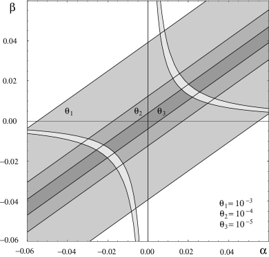
Figure 1: Constraints on the parameters $\alpha$ and $\beta$ for three different values of $\theta$. These values are $\theta_{1}=10^{-3}$, $\theta_{2}=10^{-4}$ and $\theta_{3}=10^{-5}$. The constrained region for $\alpha$ and $\beta$ is restricted by the contour curves parameterized by $\theta$ and the hyperbolic curves denoting the favoured region for a variation of the fine structure according to Webb et al..

According to recent observations, at a redshift of about one, the expansion of the universe starts to accelerate bridle . This will modify the evolution of $\phi(z)$ and therefore the expected evolution of the fine-structure constant between redshift $z=1$ and $z=0$. The details of the evolution of $\alpha_{EM}$ depend on whether or not the moduli fields have a potential and if they drive the apparent expansion at low redshift. Inferring the evolution of $\alpha_{EM}$ as a function of redshift can therefore give not only information about couplings between the moduli field(s) but also about the potential Wetterich 1 ,Wetterich 2 . When a potential for the moduli field is generated by an effective detuning of the brane tension, this leads to a variation of the cosmological constant

$$\frac{\delta\Lambda}{\Lambda}=\frac{3}{8}\frac{\alpha}{\beta}\frac{\delta\alpha_{EM}}{\alpha^{2}_{EM}},$$ (21)

in the matter dominated era. For $\beta\approx\alpha$ this implies that the variation of the cosmological constant is much smaller than the cosmological constant itself.

Finally, we consider the evolution of the ratio $\mu=m_{p}/m_{e}$. If we replace the variation of $\psi$ in terms of its cosmological evolution we obtain from (14)

$$\frac{\delta\mu}{\mu}=\frac{1}{6}\,\frac{2\pi}{b^{SM}_{3}}\frac{4\alpha\beta}{1+2\alpha^{2}}\ln(1+z).$$ (22)

Since $b^{SM}_{3}$ is negative, the variation of $\mu$ is increasing in terms of $z$. This result does not agree with the observations of Ivanchik et al. who have measured a variation $\delta\mu/\mu=(5.02\pm 1.82)\times 10^{-5}$ mp/me 1 -mp/me 2 . However, as claimed by this group, a more conservative position should be adopted until more accurate measurements come. With this caveat, the observation of a variation of $\mu$ can be taken to be $|\delta\mu/\mu|<8\times 10^{-5}$. In terms of the brane moduli parameters, this constraint gives us $|\alpha\beta|<1\times 10^{-4}$, which is compatible but stronger than the above results. We would like to emphasize again the fact that in the class of theories that we are presently considering the sign of the variation $\delta\mu/\mu$ is the same one of $\delta\alpha/\alpha$ (see equation (14)).

To summarize, in this paper we have presented two main results: firstly, we have verified that the variation of coupling parameter is frame-independent at the one-loop level in the quantum correction. Secondly, we have investigated the time variation of coupling parameter in the fairly general brane-world model with two boundary branes and bulk scalar field, whose low energy dynamics is governed by two moduli fields US . The existence of these fields leads to corrections to general relativity. We have argued that the only way to obtain time varying gauge couplings is by coupling the gauge fields directly to the bulk scalar field and allowing scalar field-dependent Yukawa couplings. We have not considered the latter possibility and analyzed a theory with two free parameters, $\alpha$ and $\beta$. The parameter $\alpha$ defines the coupling of the brane tension to the bulk scalar field while $\beta$ describes the dependence of coupling parameter to the moduli field (see equation (16)). Interestingly, both parameters, although a priori independent, have the same order of magnitude, when the current constraints of variations of the fine structure constant and current constraints by gravity experiments are considered. Our work emphasizes once more the importance of experiments looking for deviation to general relativity. Together with measurements of the fine structure constant at high redshifts this would provide useful constraints on theories beyond the standard model. In fact, for $\alpha=\beta$ in the model discussed here, violations to general relativity should be measurable very soon, if the variation of $\alpha_{EM}$ reported in Webb 1 –Webb 3 is confirmed by future investigations.

- (1) Ph. Brax and C. van de Bruck, Class. Quantum Grav. 20, R201 (2003); D. Langlois, Prog. Theor. Phys. Suppl. 148, 181 (2003).
- (2) X. Calmet and H. Fritzsch, Phys. Lett. B 540, 173 (2002); hep-ph/0211421; Eur. Phys. J.C 24, 639 (2002).
- (3) Ph. Brax, C. van de Bruck, A.C. Davis and C.S. Rhodes, Astrophys. Space Sci. 283, 627 (2003).
- (4) T. Damour, F. Piazza and G. Veneziano, Phys. Rev. D 66, 046007 (2002); Phys. Rev. Lett. 89, 081601 (2002).
- (5) C. Wetterich, hep-ph/0203266.
- (6) T. Dent and M. Fairbairn, Nucl. Phys. B 653, 256 (2003).
- (7) T. Dent, hep-ph/0305026.
- (8) V.A. Kostelecky, R. Lehnert and M.J. Perry, astro-ph/0212003.
- (9) J.P. Uzan, Rev. Mod. Phys. 75 403 (2003).
- (10) Ph. Brax, C. van de Bruck, A.C. Davis and C.S. Rhodes, Phys. Rev. D 67, 023512 (2003).
- (11) Y. Fujii and K. Maeda, The Scalar-Tensor Theory of Gravitation, Cambridge University Press (2003).
- (12) Ph. Brax and A.C. Davis, Phys. Lett. B 497, 289 (2001).
- (13) A. Lukas, B.A. Ovrut, K. Stelle and D. Waldram, Phys. Rev. D 59, 086001 (1999).
- (14) T.M. Eubanks et al., Am. Phys. Soc. K11.05, (1997).
- (15) C. Will, Living Rev. Relativ. 4, 4 (2001).
- (16) J. Webb, M. Murphy, V. Flambaum, V. Dzuba, J. Barrow, C. Churchill, J. Prochaska and A. Wolfe, Phys. Rev. Lett. 87, 091301 (2001).
- (17) J. Webb, M. Murphy, V. Flambaum, S.J. Curran, Astrophys. Space Sci. 283, 565 (2003).
- (18) M. Murphy, J. Webb, V. Flambaum, S.J. Curran, Astrophys. Space Sci. 283, 577 (2003).
- (19) S. Bridle, O. Lahav, J.P. Ostriker and P.J. Steinhardt, Science 299, 1532 (2003).
- (20) C. Wetterich, Phys. Lett. B 561, 10 (2003); C. Wetterich, hep-ph/0302116.
- (21) A.Y. Potekhin, A.V. Ivanchik, D.A. Varshalovich, K.M. Lanzetta, J.A. Baldwin, G.M. Williger and R.F. Carswell, Astrophys. J. 505, 523 (1998).
- (22) A. Ivanchik, P. Petitjean, E. Rodriguez and D. Varshalovish, Astrophys. Space Sci. 283, 583 (2003).