Long-term study of water masers associated with Young Stellar Objects. II: Analysis

We present the analysis of the properties of water maser emission in 14 star forming regions (SFRs), which have been monitored for up to 13 years with a sampling rate of about once every 2-3 months. The 14 regions were chosen to span a range in luminosity $L_{\rm fir}$ of the associated Young Stellar Object (YSO) between 20 L_⊙ and $1.8\times 10^{6}$ L_⊙. The general scope of the analysis is to investigate the dependence of the overall spectral morphology of the maser emission and its variability on the luminosity of the YSO. We find that higher-luminosity sources tend to be associated with stronger and more stable masers. Higher-luminosity YSOs can excite more emission components over a larger range in velocity, yet the emission that dominates the spectra is at a velocity very near that of the molecular cloud in which the objects are embedded. For $L_{\rm fir}$ $\;\lower 2.58334pt\hbox{$\sim$}\kern-7.75pt\raise 2.79857pt\hbox{$>$}\;3\times 10^{4}$ L_⊙ the maser emission becomes increasingly structured and more extended in velocity with increasing $L_{\rm fir}$. Below this limit the maser emission shows the same variety of morphologies, but without a clear dependence on $L_{\rm fir}$ and with a smaller velocity extent. Also, for sources with $L_{\rm fir}$ above this limit, the water maser is always present above the 5$\sigma$-level; below it, the typical 5$\sigma$ detection rate is 75-80%. Although the present sample contains few objects with low YSO luminosity, we can conclude that there must be a lower limit to $L_{\rm fir}$ ($\;\lower 2.58334pt\hbox{$\sim$}\kern-7.75pt\raise 2.79857pt\hbox{$<$}\;430$ L_⊙), below which the associated maser is below the detection level most of the time. These results can be understood in terms of scaled versions of similar SFRs with different YSO luminosities, each with many potential sites of maser amplification, which can be excited provided there is sufficient energy to pump them, i.e. the basic pumping process is identical regardless of the YSO luminosity. In SFRs with lower input energies, the conditions of maser amplification are much closer to the threshold conditions, and consequently more unstable.

We find indications that the properties of the maser emission may be determined also by the geometry of the SFR, specifically by the beaming and collimation properties of the outflow driven by the YSO.

For individual emission components the presence of velocity gradients seems to be quite common; we find both acceleration and deceleration, with values between 0.02 and 1.8 km s^-1 yr^-1.

From the 14 ‘bursts’ that we looked at in some detail we derive durations of between 60 and 900 days and flux density increases of between 40% and $\;\lower 2.58334pt\hbox{$\sim$}\kern-7.75pt\raise 2.79857pt\hbox{$>$}\;1840$% (with an absolute maximum of $\sim 820$ Jy over 63 days). The ranges found in burst- intensity and -duration are biased by our minimum sampling interval, while the lifetime of the burst is furthermore affected by the fact that bursts of very long duration may not be recognized as such.

In addition to the flux density variations in individual emission components, the H₂O maser output as a whole is found to exhibit a periodic long-term variation in several sources. This may be a consequence of periodic variations in the wind/jets from the exciting YSO.

1 Introduction

In Paper I of this series (Valdettaro et al. paper1 (2001)) we presented the results of more than 10 years of single-dish monitoring of the H₂O maser emission in 14 Star Forming Regions (SFRs) obtained with the Medicina 32-m radiotelescope. The average time interval between two successive observations is 2$-$3 months, so that our database allows one to study only the long-term ($>$ 2$-$3 months) aspects of the maser variability. For each source a brief description of the maser environment was given in Paper I, emphasizing what is of interest in the discussion of the H₂O maser variability. Here we present quantitative results derived from the long-term monitoring.

The amount of information collected on the H₂O maser emission during our study is exceedingly large. To compress it to a more manageable form the following quantities were derived (see also Paper I):

1. The flux density $F$ as a function of both velocity and time, presented in velocity-time-intensity plots, which give the best overall description of the maser activity and help to visually identify possible velocity drifs of the emission;

2. The integrated flux density $S$ as a function of time, which describes the variation of the total maser emission;

3. The upper and the lower envelopes of the spectra over the whole period of observation, obtained by assigning to each velocity channel respectively the maximum (if $>5\sigma$), and minimum (=0, unless it’s $>5\sigma$) signal detected during the monitoring period;

4. The potential maximum maser luminosity $L_{\rm H_{2}O}^{\rm up}$, derived by integration of the upper envelope. This quantity represents the maximum output which the source could produce if all the velocity components were to emit at their maximum level and at the same time;

5. The actually observed maximum maser luminosity $L_{\rm H_{2}O}^{\rm max}$, derived from the spectrum with the highest integrated flux density;

6. The frequency of occurrence of a spectral feature. To produce these plots the spectra were re-binned with a velocity resolution $\Delta V\simeq 0.3$ km s^-1, and for each channel a counter was increased by one every time the flux density in that channel was greater than 5$\sigma$;

7. The first moment of the upper envelope, $V_{\rm up}$, i.e. the average velocity weighted by the flux density, with its second moment $\Delta V_{\rm up}$, and the first moment of the frequency-of-occurrence, $V_{\rm fr}$, i.e. the average velocity weighted by the number of times that velocity component is present in the spectra, with its second moment $\Delta V_{\rm fr}$.

Since one of our main aims is to reveal aspects of the H₂O maser variability that depend on the luminosity of the Young Stellar Object (YSO) exciting the maser, the selected sample covers rather uniformly a large range of (FIR) luminosities, from 20 L_⊙ to 1.8 10⁶ L_⊙, which brackets almost the entire luminosity interval of the exciting sources of H₂O masers in SFRs (Palagi et al. PCC93 (1993); Wilking et al. wilking (1994); Furuya et al. furuya01 (2001), furuya03 (2003)).

In Table 1 we present the source sample as described in Paper I, ordered in terms of increasing FIR luminosity: Col. 1 gives the sequential number as given in Table 1 of Paper I; Cols.  2 and 3 give source names and the associated IRAS source; Cols. 4 and 5 list the B1950 coordinates; in Cols. 6 to 8 we give the radial velocity relative to the LSR ($V_{\rm cl}$) of the molecular cloud in which the SFR is embedded, the distance ($d$), and the FIR luminosity ($L_{\rm fir}$) of the source; detailed references for these quantities are given in Table 1 of Paper I. Cols. 9 to 12 list: $V_{\rm fr}$, $\Delta V_{\rm fr}$, $V_{\rm up}$, and $\Delta V_{\rm up}$ respectively, while in Col. 13 we give the total integrated H₂O flux density, determined from the upper envelope, with the corresponding potential maximum maser luminosity $L_{\rm H_{2}O}^{\rm up}$ in Col. 15. Finally, Cols. 14 and 16 give the maximum integrated H₂O flux density measured during the monitoring campaign, and the corresponding H₂O luminosity $L_{\rm H_{2}O}^{\rm max}$, respectively.

Note: After publication of Paper I, we found that the gain curve used for the May 12, 1998 data was in error. We have therefore recalibrated the spectra taken on that date. Depending on source elevation, the new flux densities may be up to a factor of 3-4 smaller than what was reported previously. In Table 2 we give the new parameters of the affected spectra.

In the present paper we shall analyse the properties of the maser emission in general terms, without discussing individual sources in any great detail. For particularly interesting sources, more in-depth studies may be presented in separate papers in the future.

Table 1: The H₂O maser sample, arranged in order of increasing FIR luminosity. Main derived parameters.

Table 2: Recalibrated data for the May 12, 1998 spectra

2 General Results

Figure 1: Distribution of the velocity difference between the mean velocity ($V_{\rm up}$) of the “upper envelope” spectrum and the molecular cloud velocity ($V_{\rm cl}$), where the “upper envelope” was created from: a all spectra, b the first third, c the middle third, and d the last third of all spectra, respectively. The identification numbers of the sources (see Tab 1) in each bin are indicated.

2.1 Mean velocities

In the literature the velocity that defines the maser emission is usually taken to be that of the peak in the spectrum. More rarely, in the presence of very complex spectra with multiple peaks, an average or centroid velocity is used. Given the large changes in the spectra when observed over long periods of time, both of these definitions tend to be a function of the observing date. Consequently it is not a surprise that the velocity of the maser, as quoted in the literature, may change with time.

These maser velocities are usually compared with those of the molecular clouds in which the SFRs are embedded. The results indicate a good general agreement between the two, with a dispersion $\simeq 4-11$ km s^-1 (Wouterloot et al. wou95 (1995), Anglada et al. ang96 (1996)).

Our first-moment velocities $V_{\rm up}$ and $V_{\rm fr}$ are derived from the upper envelope and the frequency-of-occurrence plots, respectively, and refer to a long ($\sim 10$ yrs) period of observation. Consequently they offer a way to define a mean velocity of the maser emission that is less dependent on the epoch of the observation.

As indicated in Table 1, $V_{\rm up}$ and $V_{\rm fr}$ are almost identical, with a mean difference of 0.2 km s^-1 and a standard deviation of 1.2 km s^-1. This implies that the velocity at which the emission is most intense is also that where emission occurs most frequently.

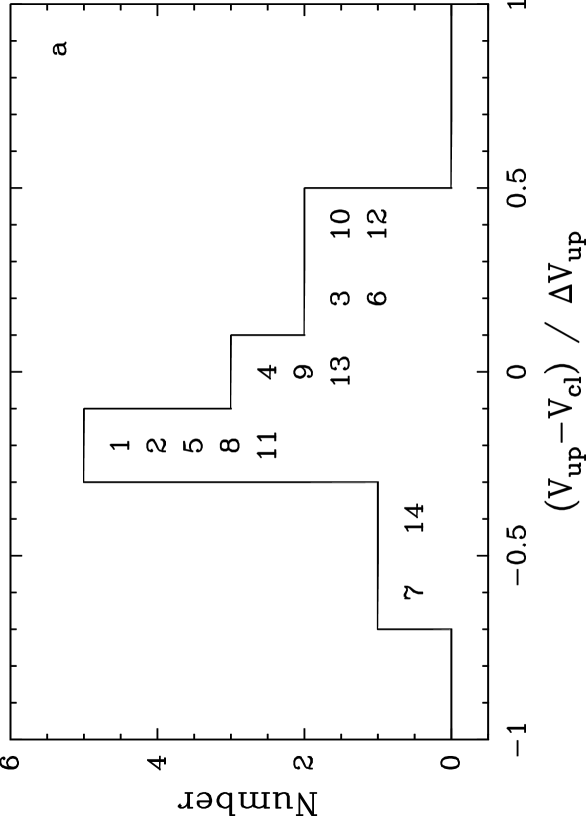
Figure 2: a Distribution of the velocity difference between the mean velocity of the “upper envelope” spectrum and the molecular cloud velocity, relative to the velocity dispersion (second moment) of the maser emission ($\Delta V_{\rm up}$). The identification numbers of the sources in each bin are indicated. b The absolute value of the parameter shown in a, as a function of the FIR luminosity of the associated YSO. The dashed line marks $L_{\rm fir}$= $3.7\times 10^{3}$ L_⊙, above which the relative velocity difference between maser and cloud seems to be smaller (see text).

It is also instructive to compare $V_{\rm up}$ or $V_{\rm fr}$ with the velocity of the molecular cloud. As shown in Fig. 1a, $|V_{\rm up}|$ differs always less than $\sim 7.5$ km s^-1 from the corresponding molecular cloud velocity, $V_{\rm cl}$. The distribution of $V_{\rm up}-V_{\rm cl}$ has a mean value of $-$0.4 km s^-1 and a standard deviation of 3.5 km s^-1, much smaller than the value of 11 km s^-1 found using the peak velocity of single-epoch H₂O maser spectra by Anglada et al. (ang96 (1996)), but similar to the 3.65 km s^-1 found by Wouterloot et al. (wou95 (1995)).

Considering the shape of the upper envelopes (see paper I and Fig. 13), the above implies that the maser emission is maximum for zero projected velocities with respect to the local environment. This confirms the well-known fact (Elitzur et al. eli89 (1989), eli92 (1992)) that the maser emission is maximum when the plane of the shocks that create the masing conditions is oriented along the line-of-sight.

There are a few sources with large values of $|V_{\rm up}-V_{\rm cl}|$ (up to $\sim$ 7 km s^-1): L1204-G (source number 14) at the negative velocity end, and NGC7129/FIRS2 (nr. 12) at the positive end. An offset between the velocity of the maser emission and that of the molecular cloud is however only significant if it is of the order of, or larger than the width of the maser emission, and if it is persistent in time. To investigate the former, we show in Fig. 2a the distribution of ($V_{\rm up}-V_{\rm cl})/\Delta V_{\rm up}$. $\Delta V_{\rm up}$ is the second moment of the upper envelope, and as such a measure of the velocity extent of the maser. For a purely Gaussian distribution, the second moment is the square of the standard deviation; for the actual shape of the upper envelopes the precise meaning of $\Delta V_{\rm up}$ is less straightforward, although it still represents a measure of the velocity dispersion of the maser. Thus, Fig. 2a shows that the velocity difference between the maser and the cloud is always less than the width of the maser emission as measured by $\Delta V_{\rm up}$. The sources with the largest negative velocity offset are G32.74$-$0.08 (number 7; ($V_{\rm up}-V_{\rm cl})/\Delta V_{\rm up}=-0.58$), and L1204-G (nr. 14; $-0.50$); the largest positive offset is for NGC7129/FIRS2 (nr. 12; 0.44). G59.78+0.06 (nr. 10), in the same bin as nr. 12, has a fractional offset of only 0.34.

Fig. 2b shows the relation of the absolute value of the difference between the maser- and cloud velocity, relative to the maser velocity width, as a function of $L_{\rm fir}$. This diagram suggests that for $L_{\rm fir}$ $\;\lower 2.58334pt\hbox{$\sim$}\kern-7.75pt\raise 2.79857pt\hbox{$<$}\;7\times 10^{3}$ L_⊙ relatively large values of $|V_{\rm up}-V_{\rm cl}|/\Delta V_{\rm up}$ may occur, while for the masers pumped by a higher-luminosity YSO the emission that dominates is at a velocity much closer tothat of the molecular cloud in which they are embedded ($|V_{\rm up}-V_{\rm cl}|/\Delta V_{\rm up}<0.2$).

To see how persistent these velocity offsets are in time, we have derived for each source the “upper envelope” spectrum separately for the first, middle, and last third of all spectra, and calculated ($V_{\rm up}-V_{\rm cl}$) in each case. The resulting distributions are shown in Figs. 1b, c, and d. From these histograms we see that with time the three extreme cases identified from Fig. 2a move to the lower bins, i.e. the difference between the mean maser velocity and the molecular cloud velocity becomes progressively smaller for all three sources. For L1204-G (nr. 14) this is because the (more intense) blue-shifted maser lines become redder with time, while the red-shifted components become bluer (see Paper I: Fig.29); for G32.74$-$0.08 (nr. 7), while the main emission remains significantly displaced bluewards of the molecular cloud velocity, red-shifted components appear which shift $V_{\rm up}$ towards $V_{\rm cl}$ (Paper I: Fig. 15); in NGC7129/FIRS2 (nr. 12; Paper I: Fig.25) the whole of the maser emission gradually shifts towards the blue (and towards $V_{\rm cl}$) with time.

From a closer look at these data it appears that a variation in the overall width of the maser emission is anti-correlated with a variation in its velocity. This is brought out clearly in Fig. 3, where we show the maximum change in $\Delta V_{\rm up}$ during the three time intervals considered, relative to the $\Delta V_{\rm up}$ derived from all spectra, as a function of the maximum change in the velocity difference during those time intervals. Masers that during monitoring have undergone a large change in one of those parameters have changed little in the other.

Figure 3: The maximum change in $\Delta V_{\rm up}$ during the three time intervals considered (see text), relative to the $\Delta V_{\rm up}$ derived from all spectra, as a function of the maximum change in the velocity difference during those time intervals.

This velocity analysis shows that though individual maser components may have a large proper motion with respect to the molecular cloud in which they are embedded (e.g. Seth et al. seth (2002)), the centroid of the maser emission remains close to the cloud’s velocity and, averaged over time, reaches an offset of at most half the maser’s velocity dispersion as measured by the second moment of the “upper envelope”. There seems to be a critical value of the $L_{\rm fir}$ of the associated YSO, below which larger deviations can occur between the maser’s velocity centroid and that of the molecular cloud than above it. This result can be understood within the framework of the scenario for maser emission around a YSO that emerges in the course of this analysis, and which will become more clear after having considered other observational results (in particular in Sects. 2.3, 2.4, 2.5, 2.8.3, and 2.8.4). We assume that around a YSO there are many potential maser sites, that can be excited by impact with an outflow originating at the YSO if the appropriate masing conditions can be created. This will be seen to also depend on the directional properties of the outflow. High-luminosity YSOs may consist of a collection of lower-luminosity objects, all of which can have an associated outflow, pointing in different directions, giving rise to a higher degree of isotropy of the maser emission emanating from the SFR. Lower-luminosity YSOs, on the other hand, could either be single objects, or less numerous collections of even lower-luminosity sources. In a SFR with smaller $L_{\rm fir}$, there will therefore be fewer outflows, and these will be less powerful than in the high-luminosity SFRs. Fewer maser sites will be excited, and the emerging maser emission will be more anisotropic in this case. The velocity at which one detects the maser emission will in this case depend more on the local morphology of the SFR and on the orientation of the outflows, and can deviate more from $V_{\rm cl}$ than in the high-luminosity case.

2.2 Maser luminosity

Figure 4: Far-infrared- vs. H₂O luminosity for the sample of 14 sources. The drawn line is a least-squares (bisector) fit to the $L_{\rm H_{2}O}^{\rm up}$ data points (large circles; the numbers identify the sources, see Table 1); the dotted line fits the $L_{\rm H_{2}O}^{\rm max}$ data (small empty circles, each below the corresponding large circle); the dashed line represents the fit reported by Wouterloot et al. (wou95 (1995)).

Previous attempts to correlate the maser luminosity with the FIR luminosity of the associated YSO have always dealt with instantaneous maser spectra (Palagi et al. PCC93 (1993); Wouterloot et al. wou95 (1995)). Given the high variability of the maser emission that we find in almost all sources, the instantaneous maser luminosity is also highly variable (cf. Fig. 15). This may produce two effects: 1) it might obscure any possible correlation existing between the luminosity of the YSO that powers the maser, and the maser luminosity, and 2) it might lead one to strongly underestimate the conversion factor from YSO luminosity to maser luminosity.

For this reason the maximum H₂O maser luminosity $L_{\rm H_{2}O}^{\rm up}$, derived from the upper envelope spectra, should represent a more reliable estimate of the potential emission of the H₂O maser since it eliminates the effects of the variability of the individual velocity components. $L_{\rm H_{2}O}^{\rm up}$ better approximates the maximum maser emission since it gives what the maser would emit if all the velocity components were active at their maximum level and at the same time.

$L_{\rm H_{2}O}^{\rm up}$  correlates well with the FIR luminosity of the YSO (Fig. 4). The best fit (drawn line) to the data points (encircled numbers) gives log[$L_{\rm H_{2}O}^{\rm up}$] = ($-7.20\pm 0.35)+(0.81\pm 0.07$)log[$L_{\rm fir}$] (corr. coeff. 0.80), i.e. $L_{\rm H_{2}O}^{\rm up}$  = $6.37\times 10^{-8}L_{\rm fir}^{0.81\pm 0.07}$. This fit agrees reasonably well with that obtained by Wouterloot et al. (wou95 (1995); represented by the dashed line: $L_{\rm H_{2}O}$ = 4.47$\times 10^{-8}L_{\rm fir}^{1.00\pm 0.07}$), as could be expected since our data base contains many observations of a small number of objects, while theirs consists of few observations of many objects. As can be seen from Fig. 7 in Wouterloot et al., at constant $L_{\rm fir}$ the water maser luminosity can change over up to 4 orders of magnitude, which affects the luminosity derived from instantaneous observations, and may be explained by changes in the direction of the maser beam and/or changes in the maser excitation and amplification (see also Elitzur elitzur (1992)).

By its definition, the maser luminosity derived from the upper envelope represents an upper limit to the instantaneous maser luminosity. In Fig. 4 we therefore also show the fit to $L_{\rm H_{2}O}^{\rm max}$, which is derived from the actually observed maximum integrated flux density. This fit is described by $L_{\rm H_{2}O}^{\rm max}$  = $2.75\times 10^{-8}L_{\rm fir}^{0.82\pm 0.08}$ (corr. coeff. 0.79), and is shown as the dotted line. As expected, it lies below the relation defined by $L_{\rm H_{2}O}^{\rm up}$ (by $\sim 0.4$ in log[L${}_{H_{2}O}$]). We find $L_{\rm H_{2}O}^{\rm max}$/$L_{\rm H_{2}O}^{\rm up}$ to be between 0.25 (Sh 2-269 IRS2; source nr. 5) and 0.80 (Mon R2 IRS3; nr. 4); there is no correlation between this ratio and $L_{\rm fir}$.

2.3 A variability index for the maser emission

The definition of a variability index to describe with a single parameter the variability of a maser (or even a single emission component) is an almost impossible enterprise in view of the complex patterns shown in the velocity-time-intensity plots (paper I and Fig. 11). With these limitations, and aiming to capture the overall variation of the maser emission, we have derived for each source the ratio $S_{\rm max}$/$S_{\rm mean}$ between the maximum and the mean integrated flux densities over the whole monitoring period. An anti-correlation is found between the YSO FIR luminosity and this ratio (Fig. 5). Clearly, high-luminosity sources tend to be associated with more stable masers, while lower luminosity ones have a more variable emission. Note that L1455 IRS1 (source nr. 2), the maser emission of which often disappears below our detection limit, appears twice in Fig. 5, because $S_{\rm mean}$ was calculated in two ways: by assigning to the non-detections either a value of 0 (resulting in the higher value of the plotted ratio) or $3\sigma(V_{\rm max}-V_{\rm min})$ (resulting in the lower value of the plotted ratio), where $V_{\rm max}$ and $V_{\rm min}$ are the extreme velocities of the corresponding upper envelope spectrum, and $\sigma$ is the rms-noise in an individual maser spectrum.

In lower-luminosity YSOs a smaller number of maser components gets excited (see also Sect. 2.5) and their intrinsic time-variability will affect the total output more than in higher-luminosity YSOs, where a much larger number of components might be simultaneously excited, thus reducing the effect of their individual time-variability on the total maser output. Moreover, for increasingly smaller $L_{\rm fir}$, the conditions of maser amplification are more likely to be closer to the threshold conditions and consequently the maser emission will be more unstable.

Figure 5: Ratio between the maximum integrated flux density ever observed, $S_{\rm max}$, and the mean value of the integrated flux density, $S_{\rm mean}$, over the whole monitoring period, as a function of the YSO FIR luminosity. The two appearances of object nr. 2 (L1455 IRS1) represent different ways to take into account the numerous non-detections of the maser (see text).

2.4 Velocity range of the maser emission

In order to characterize the velocity width of the emission we use the second moment of the “upper envelope” spectrum, $\Delta V_{\rm up}$.

$\Delta V_{\rm up}$ is shown as a function of the YSO FIR luminosity in Fig. 6. It seems that high values of $\Delta V_{\rm up}$ are encountered only for high $L_{\rm fir}$, while lower $\Delta V_{\rm up}$ values occur at any FIR luminosity. Thus, more luminous sources can excite maser emission over a larger velocity interval, but apparently do not necessarily always do so. Therefore, what the upper envelope shows is potential. Rather than showing a relation between the data points, Fig. 6 defines an upper boundary indicating that there is a maximum possible velocity extent of the maser emission, which depends on the FIR luminosity of the associated (pumping-) source. This upper limit is shown in Fig. 6 as a dashed line, defined by the sources 2, 6, 8, 12, 13, and 14: $\Delta V_{\rm up}\propto L_{\rm fir}^{4.68\pm 0.26}$.

Felli et al. (FPT92 (1992)) found a correlation between the maser luminosity and the mechanical luminosity of the associated molecular outflow (see also Lada lada85 (1985)), supporting the hypothesis that maser conditions are created where the molecular outflows shock the surrounding molecular gas. The mechanical luminosity of the outflows is also correlated with the FIR luminosity of the YSOs. Similarly, Wouterloot et al. (wou95 (1995)) found that for $L_{\rm fir}$$>10^{2}$ L_⊙ IRAS sources with “maser-like” colours have significantly larger CO (FWHM) linewidths than those with “non-maser-like” colours, and that this is even independent of whether a maser has actually been detected or not. The CO (FWHM) linewidth was found to depend only weakly on $L_{\rm fir}$: an increase of a factor of about 2 between $L_{\rm fir}$=$10^{2}$ and $10^{6}$.

Figure 6: Plot of the second moment of the “upper envelope” spectrum as a function of the YSO FIR luminosity. The dashed line is a (bisector) least-squares fit through 6 data points defining an upper boundary to the data: $\Delta V_{\rm up}\propto L_{\rm fir}^{4.68\pm 0.26}$.

The use of $\Delta V_{\rm up}$ to characterize the velocity range of the maser emission can be misleading, however: if the maser emission is dominated by one or a few strong components, then $\Delta V_{\rm up}$ will be small, even though there may be many weaker components with a large range of velocities. These weaker outlying components are taken into account if the velocity range of the maser emission ($\Delta V_{\rm tot}$) is taken to be the total velocity extent in the frequency-of-occurrence histograms (see Paper I and Fig. 14). The general trend is that $\Delta V_{\rm tot}$ increases with $L_{\rm H_{2}O}^{\rm up}$, $L_{\rm H_{2}O}^{\rm max}$, and $L_{\rm fir}$. As an example we show this for $L_{\rm H_{2}O}^{\rm up}$ in Fig. 7.

Figure 7: Total velocity range of the maser emission, $\Delta V_{\rm tot}$ determined from the frequency-of-occurrence histograms, as a function of $L_{\rm H_{2}O}^{\rm up}$. The dashed line is a (bisector) least-squares fit through 4 data points defining an upper boundary to the data: $\Delta V_{\rm tot}$ = (168.1 $\pm$ 4.5) + (27.12 $\pm$ 1.08)log$L_{\rm H_{2}O}^{\rm up}$.

Just like Fig. 6, Fig. 7 shows that while in stronger maser sources (associated with more luminous YSOs, see Fig. 4) emission can be excited over a larger range in velocity, there is no guarantee that this will be so: many of the more luminous objects have a relatively small $\Delta V_{\rm tot}$. An example is Sh 2-269 IRS2 (source nr. 5), where the maser emission, while strong, is always contained within a rather narrow velocity interval (at least at the 5$\sigma$-level used to construct the frequency-of-occurrence histograms). A different case is Mon R2 IRS3 (nr. 4), a strong maser with emission virtually always in a very narrow range of velocities (see Paper I, Fig. 9), but which during our long monitoring campaign occasionally showed components both blue- and red-shifted by up to 20 km s^-1, thus increasing $\Delta V_{\rm tot}$. Thus, also in Fig. 7 the data points define an upper boundary indicating the maximum possible velocity range of the maser emission as a function of $L_{\rm H_{2}O}^{\rm up}$. In Fig. 7 this envelope is determined by sources 2, 4, 8, and 13. A bisector fit through these data points gives $\Delta V_{\rm tot}$ = (168.1 $\pm$ 4.5) + (27.12 $\pm$ 1.08)log$L_{\rm H_{2}O}^{\rm up}$, which is shown as a dashed line. Note that the value of the intercept is influenced by the sensitivity of the data, by the 5$\sigma$ detection limit adopted in the construction of the frequency-of-occurrence histograms, as well as by the fact that there may be emission at velocities not within our frequency band (see the velocity-time-intensity diagrams in Paper I).

2.5 Distribution of velocity components

Our single-dish observations can resolve the maser emission only in the velocity domain, but not in the spatial domain. Interferometric observations (see e.g. VLBA observations by Seth et al. seth (2002)) have shown that a single velocity component may arise from as many as a dozen spatially separated maser spots. With the provision that the number of spectral components observed in our spectra does not necessarily correspond directly to the number of individual maser components present in the SFR, by studying their distribution in velocity we can still derive useful information on how the energy input from one or more YSOs in a SFR is distributed in the outcoming maser spectrum, and how the situation is affected by the luminosity of the YSOs, or, ultimately, how the dynamics of the molecular cloud surrounding the YSOs is affected by their presence.

To study this effect we used the spectrum with the highest integrated flux density during the monitoring period, in which we have counted the number of individually visible spectral components, including emission down to levels of $2-3\sigma$ (which however varies from spectrum to spectrum). (This is practically impossible to do from either the upper envelope spectrum or the frequency-of-occurrence histograms, where the individual components appear indistinguishably merged due to (random and systematic) velocity shifts during the monitoring period.) In Fig. 8 we plot for each source the number of components in the spectrum with the maximum integrated flux density as a function of the total velocity range of the emission in that spectrum. Note that both quantities plotted are lower limits, due to a combination of sensitivity, spectral resolution, and the intensity of individual components. Nevertheless, there is a clear and rather tight correlation between the number of components in a spectrum and the velocity range over which they are found. A bisector fit through all data points gives the number of components, $Nc$, as a function of velocity range, $Vrange$: $Nc=(1.2\pm 0.4)+(0.30\pm 0.02)\leavevmode\nobreak\ Vrange$ (corr. coeff. 0.97). One way of looking at this relation is that for every 10 km s^-1 increase in $Vrange$, three more components are found.

Figure 8: The number of emission components, $Nc$, in the spectrum with the highest integrated flux density, as a function of the velocity range of the emission, $Vrange$, in that spectrum. The drawn line is a (bisector) least-squares fit to all data points: $Nc=(1.2\pm 0.4)+(0.30\pm 0.02)\leavevmode\nobreak\ Vrange$

Figure 9: Correlation between the number of components (a) and the velocity range of the maser emission (b) in the spectrum with the highest integrated flux density, as a function of $L_{\rm H_{2}O}^{\rm max}$, the maser luminosity determined from that same spectrum. Both quantities increase with increasing maser luminosity.

The number of components and the velocity range are plotted separately as a function of $L_{\rm H_{2}O}^{\rm max}$ in Fig. 9a and b, respectively. We see that both quantities increase with increasing maser luminosity.

Note that in Fig. 9b we find a correlation between $Vrange$ and $L_{\rm H_{2}O}^{\rm max}$, rather than just an upper boundary, as was the case for $L_{\rm H_{2}O}^{\rm up}$. This is because $L_{\rm H_{2}O}^{\rm max}$ is directly related to the velocity range, in the sense that it pertains to the same spectrum, while $L_{\rm H_{2}O}^{\rm up}$, which measures some fictitious maximum maser luminosity, can be anywhere between 1.25 and 4 times larger than $L_{\rm H_{2}O}^{\rm max}$ (see Sect. 2.2).

Figures 8 and 9 show that higher maser power goes into more emission channels, that are spread over a larger range in velocity. Both the number of components and the velocity range of the emission seem to be insensitive to $L_{\rm fir}$ (not shown): higher $L_{\rm fir}$ allows a larger velocity extent of the maser emission, but does not impose it. As a consequence, and perhaps surprisingly, the maximum velocity range (and the largest number of components) are not necessarily reached in the spectrum with the largest integrated flux density.

In a SFR there are likely to be many potential sites of maser amplification, which can be excited if there is sufficient energy to pump them. Water masers are excited behind shocks (Elitzur et al. eli89 (1989)), which are likely to be caused by outflows or jets driven by the associated YSO (Felli et al. FPT92 (1992)). To excite maser emission at large (relative to the ambient molecular cloud) velocities requires sufficiently powerful jets and outflows from the YSO to provide the necessary energy. Hence, the more luminous YSO’s will be associated with maser spectra containing more emission components over a larger range in velocity, as we indeed find. The basic pumping process seems to be the same regardless of the YSO luminosity, but in SFRs with lower input energies (i.e. a lower YSO-luminosity driving a lower-velocity outflow) only components with low (relative to the ambient molecular cloud) velocities can be excited.

2.6 Velocity drifts

In all sources, most if not all spectral features undergo velocity drifts, and a number of them have been identified in Paper I. These can be recognized in the large scale velocity-time-intensity plots of Paper I as inclined linear structures, indicating systematic changes of line-of-sight velocity of the masing gas with time.

Indirect evidence that velocity drifts must be observable in maser components comes also from VLBI observations (e.g. Seth et al. seth (2002)). From studies of the spatial distribution and proper motions of maser spots, three type of maser components are found: 1) in a rotating disk around the YSO; 2) in a high-velocity collimated bipolar outflow originating from the YSO and perpendicular to the disk; and 3) at the bow shocks produced by the outflows. Velocity drifts can occur due to rotation of the disk, to acceleration or decelaration in the collimated outflow, or to precession of the jet/outflow. One does not need high spatial resolution to study these velocity drifts, as they are observable also with single-dish monitoring of the type presented in this work (e.g. Cesaroni cesa (1990); Lekht et al. lekht140 (1993)).

With a spectrum every 2–3 months (i.e. once every $\sim 60-100$ days), and a spectral resolution of $\sim 0.16$ km s^-1, the minimum detectable velocity drift from spectrum to spectrum is $\;\lower 2.58334pt\hbox{$\sim$}\kern-7.75pt\raise 2.79857pt\hbox{$>$}\;0.6-1.0$ km s^-1 yr^-1. However, if a component can be traced over a longer period of time, then the minimum detectable value can be much less than this. In fact, for the 15 emission components that we have analyzed we find velocity gradients between 0.02 and 1.8 km s^-1 yr^-1. The lower value is found for components that could be traced over the whole $\sim 4600$ day period of monitoring, while the higher value was found for a burst-component with a duration of $\sim 63$ days. Considering the small number of components studied in detail, we find equal numbers of negative (9/15) and positive (6/15) velocity gradients.

Since the intensity of the velocity component during the drift is far from constant, one might object that what we see is not due to a unique component drifting in velocity, but rather to a casual sequence of small bursts each one occuring at a slightly different velocity and with the proper time delay with respect to the preceeding one, as the short time-duration of the spatial-velocity components found by Seth et al. (seth (2002)) from VLBA observations might suggest. Obviously, we have no means to reject this second explanation and we believe that in the spectra of sources which have a large number ($>$10) of velocity components bursting in a random fashion it is impossible to make any statement of this type. Another difficulty arises from the fact that many features have very short life-times and in such small time interval ($\sim$ one year) the effect of a velocity drift may be less evident.

This is why we have limited ourselves to the most obvious cases, in particular to sources with few velocity components, to sources in which one component dominates the spectrum, or to sources with components at velocities far from the more crowded part of the spectrum. One of the best examples is L1204-G (Fig. 10) where at least four components (two around $-$19 km s^-1, one near $-$10 km s^-1, and one at $-$2.5 km s^-1) are seen drifting in opposite directions almost throughout the entire monitoring period. For the $-$2.5 km s^-1 component we derive a velocity drift of $-0.10$ km s^-1 yr^-1 for the first $\sim 1500$ days after its first detection, followed by a more rapid deceleration of $-0.40$ km s^-1 yr^-1 in $\sim 680$ days (associated with an increase of this component’s flux density from 2 to 20 Jy). The $-$19 km s^-1 components changes velocity in a more erratic way: while the general trend is for the velocity to become redder, there are periods in which the velocity is constant or becomes bluer. The $-$10 km s^-1 component shows a velocity gradient of $+1.23$ km s^-1 during the first $\sim 790$ days after its first appearance around day 1850 ($+0.57$ km s^-1 yr^-1); after reaching a peak in flux density of $\sim 50$ Jy on day 2243 it rapidly dropped below our detection limit, only to resurface near the end of the monitoring period (in the last spectrum $F\approx 97$ Jy), with a velocity that agrees with an extrapolation of the gradient found from its previous appearance. In Fig. 10 we also see a component at $V_{\rm lsr}$$\simeq-24$ km s^-1, near day=3000. In the 6 observations taken around that date (day 2879$-$3083), the line exhibits a redshift of 0.7 km s^-1 yr^-1; including also the observation at day=2711, the redshift amounts to 1.8 km s^-1 yr^-1. The velocity-change coincides with a period of decline after an increase in flux density.

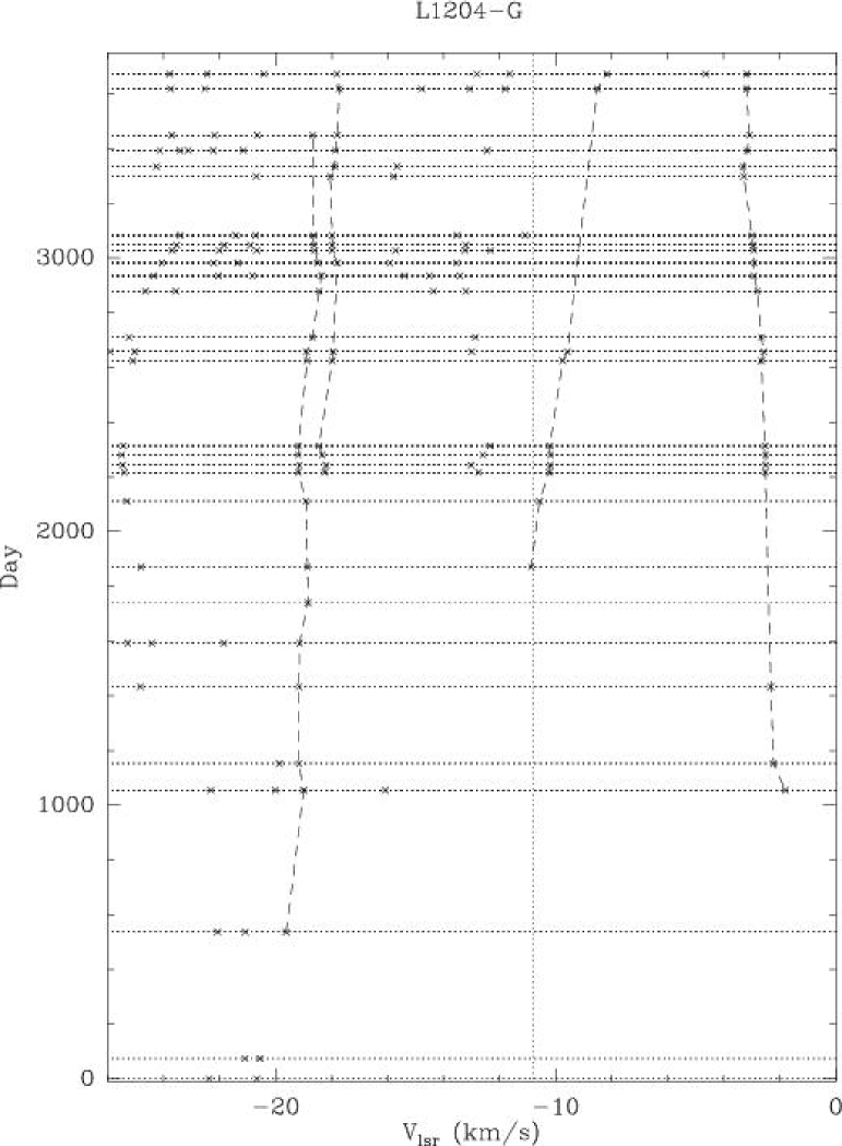
Figure 10: Overview of the velocity of the emission components in L1204-G spectra, derived from Gaussian fits. The horizontal dotted lines indicate the days (averaged in bins of 10 days) for which spectra are available; the vertical dotted line indicates the velocity of the surrounding high-density molecular gas ($V_{\rm cl}$). The crosses mark the central velocity of each fitted emission peak; Velocities considered to identify single components are connected by a dashed line, if they are visible over a considerable amount of time.

A behaviour similar to that found for the $-2.5$ km s^-1 component in L1204-G has been found in W75N by Hunter et al. (hun94 (1994)) who interpreted the drift as an outward acceleration. Likewise, the reddening of the components at $-19$ and $-10$ km s^-1 could be taken as an outward acceleration of maser features on the far side of the driving source. However, as summarized at the beginning of this sub-section, other explanations are possible, including precession of the jet exciting the maser, and rotation of the maser component around the YSO, as well as random superposition of short bursts of spatially separated components at similar velocities, even though it seems improbable that this explanation might work for steady drifts persisting over many years. Only a finer time-sampling of single-dish observations together with frequent VLBI observations can clarify this issue.

2.7 Maser bursts: duration, intensity and linewidth

A burst is a rapid increase of the flux density of the maser emission at a given velocity $V$ during a certain (usually brief) time. The change in flux density is defined as $\Delta F(V)=[F_{\rm peak}(V)-F_{\rm steady}(V)]$, where $F_{\rm steady}(V)$ is the (average of the) intensity level immediately before and after the burst at velocity $V$. During the burst, the flux density reaches a maximum $F_{\rm peak}(V)$. The burst’s duration is $\Delta t(V)=[t_{\rm final}(V)-t_{\rm initial}(V)]$, where $t_{\rm initial}(V)$ and $t_{\rm final}(V)$ denote the time of start and end of the flux density increase, respectively.

Given the variability of the emission and the relatively long time between two consecutive observations, it is often difficult to determine these parameters, and the determination of $\Delta F(V)$ and $\Delta t(V)$ is not homogeneous and rather subjective. The ever-present intrinsic variability can make it difficult to distinguish a burst, unless the increase in flux density is particularly large with respect to the ‘normal’ variability. $\Delta t(V)$ depends on the rapidity of the flux density change, shorter bursts being easier to isolate. Finally, a proper determination of $\Delta t(V)$ is influenced by the uneven time coverage of our monitoring, and by the minumum sampling interval. Hence, $\Delta F(V)$ tends to be a lower limit, $\Delta t(V)$ an upper limit.

We have not done any systematic analysis of bursts, but as with the analysis of velocity gradients in the previous sub-section we have selected a few of the more evident examples: we selected 14 bursts in 9 emission components, in 6 sources. In this small sample we find increases of flux density ($\Delta F(V)$) from about 40% to $\;\lower 2.58334pt\hbox{$\sim$}\kern-7.75pt\raise 2.79857pt\hbox{$>$}\;1840$% with respect to the $F_{\rm steady}(V)$-level; the largest absolute flux density increase was found in Mon R2 ($\sim 820$ Jy [75%], in a burst lasting 63 days). $\Delta t(V)$ ranges from a minimum value equal to our sampling interval ($\sim 60$ days) to up to $\sim 900$ days, mainly because variations of longer duration are not defined as bursts. However, some type of long-term (‘super-’) variability is visible in the behaviour of $\int F{\rm d}v$ of several sources: the integrated flux density of all maser components changes more or less regularly with time. We will discuss this long-term variability in Sect. 2.8.5.

For W49N, Liljeström & Gwinn (lil00 (2000); their Fig. 10) find that the duration and intensity of the maser outbursts depend on the velocity offset with respect to $V_{\rm up}$: high-velocity blue-shifted and red-shifted components seem to have shorter duration and smaller flux density increase than those close to $V_{\rm up}$. We do see an indication for this from the shapes of the upper envelopes (see Paper I and Fig. 13) of our sources, in which the flux density tends to decrease very rapidly at velocities away from $V_{\rm up}$. At the same time the frequency-of-occurrence diagrams (Paper I and Fig 14) show that maser components at large blue- and red-shifted velocities (with respect to $V_{\rm fr}\approx V_{\rm up}$) are detected only a fraction of the time, compared to the components near $V_{\rm up}$, implying that the lifetime of these maser components is shorter. It should be noted though, that weaker, short-duration components that occur in the central, most crowded part of the spectra, are virtually impossible to identify.

Clearly, the two dependencies call for a unique explanation. The geometrical one seems to be the simplest and most widely accepted: if masers occur in shocks and the peak of the maser-beaming is in the plane of the shock, then the both the maximum emission and the largest $\Delta F(V)$ will be observed from planes closely aligned with the line-of-sight, and at a line-of-sight velocity near the systemic velocity ($V_{\rm cl}$). Small changes in the amplification of the maser will produce larger absolute changes in flux density. At velocities near $V_{\rm cl}$ we are likely to see the cumulative effects of more than one maser spot, as all spots with the plane of the shock along the line-of-sight will be in the condition of maximum beaming.

Liljeström & Gwinn (lil00 (2000)) suggest that the duration of the burst is determined by the time required by the shock to propagate across the maser filament, $\Delta t(V)$ = D/V, where D is the transverse diameter of the maser. Assuming a mean value of D$\sim$1 AU and V $\sim$$<$ 55 km s^-1, which in our sample is the maximum velocity offset between a maser component and the velocity of the cloud in which it is embedded, we obtain $\Delta t(V)\;\lower 2.58334pt\hbox{$\sim$}\kern-7.75pt\raise 2.79857pt\hbox{$>$}\;32$ days, which is at the limit of our sampling rate.

This would also explain the dependence of $\Delta t(V)$ on the velocity offset. The suggestion of Liljeström & Gwinn (lil00 (2000)) is that high-velocity offsets from $V_{\rm up}$ select higher velocities in the outflow and hence higher shock velocities and smaller $\Delta t(V)$.

Another quantity that has often been discussed in relation to maser bursts is the change of the linewidth during a burst. In the (small) number of bursts investigated by us, we do not see any systematic behaviour in $\Delta V_{\rm fwhm}$ with flux density, which agrees with the Liljeström & Gwinn (lil00 (2000)) study of bursts in W49N.

2.8 Comparison of overall maser properties as a function of FIR luminosity

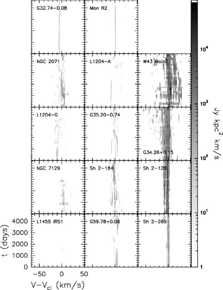
Figure 11: Grey-scale maps of the flux density, multiplied by distance²; cf. Paper I. The velocity scale is relative to the cloud velocity $V_{\rm cl}$. $L_{\rm fir}$ increases from bottom to top and from left to right; Mon R2 IRS3 has $L_{\rm fir}$$=3.2\times 10^{4}$ L_⊙.

2.8.1 The scaled velocity-time-intensity plots

In Fig. 11 we show the velocity-time-intensity plots in order of increasing FIR luminosity ($L_{\rm fir}$ increases from bottom to top, and left to right). The velocity-scale is the same in all plots and the velocities are referred to $V_{\rm cl}$ (i.e. the quantity on the horizontal axis is $V_{\rm observed}-V_{\rm cl}$). The intensity in all plots has been normalized to the same distance, by multiplying the values by (d[kpc])². The (logaritmic) intensity scale in all plots is the same so that Fig. 11 shows what one would see if all the sources were at the same distance.

Note that for $L_{\rm fir}$$\;\lower 2.58334pt\hbox{$\sim$}\kern-7.75pt\raise 2.79857pt\hbox{$>$}\;3\times 10^{4}$ L_⊙ the emission becomes increasingly complex: going from Mon R2 IRS3 ($L_{\rm fir}$$=3.2\times 10^{4}$ L_⊙) to W43 Main3 ($L_{\rm fir}$$=1.8\times 10^{6}$ L_⊙) the maser emission changes from being dominated by a single component to being highly structured and multi-component; the velocity extent of the emission also increases. For $L_{\rm fir}$$\;\lower 2.58334pt\hbox{$\sim$}\kern-7.75pt\raise 2.79857pt\hbox{$<$}\;3\times 10^{4}$ L_⊙ on the other hand, while the maser emission shows the same variety of morphologies, from the single-/dominant component-type to a (modest) degree of complexity, there is no systematic trend with $L_{\rm fir}$ and the velocity extent of the maser emission remains smaller than what is found for the highest-luminosity sources (cf. Fig. 7, Sect. 2.4). The source with the lowest $L_{\rm fir}$ (20 L_⊙; L1455 IRS1: nr. 2) is again a special case, where for much of the time the maser has not been detected. This can be understood by the explanation given for the variability in Sect. 2.3, and is consistent with the results of a 13-month maser-monitoring program of low-luminosity YSO’s by Claussen et al. (cla96 (1996)): below a YSO luminosity $L_{\rm fir}$$\sim$25 L_⊙ there is a higher degree of variability of the maser emission, which often disappears below the detection threshold.

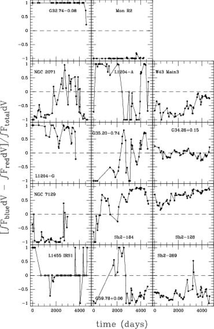
Figure 12: The normalized difference between the integrated (Jy  km s^-1) blue and red parts of the spectra of all sources, as a function of time. Integration was performed from $-\infty$ to $V_{\rm cl}$ (blue) and from $V_{\rm cl}$ to $\infty$ (red), where the reference velocity $V_{\rm cl}$ is that of the molecular cloud (see Table 1). Open circles indicate cases where both integrals are zero (i.e. no maser detection). The panels are ordered in $L_{\rm fir}$, which increases from bottom to top and from left to right.

2.8.2 Red and blue asymmetries in the spectra

In Fig. 12 we show the relative strengths of the integrated blue (integrating between $-\infty$ and $V_{\rm cl}$) and red ($V_{\rm cl}$ to $\infty$) maser emission as a function of time. The difference between the blue and red integrals is normalized by the total integrated flux. The panels are ordered in $L_{\rm fir}$ as in Fig 11. In this figure, masers with predominantly blue (red)-shifted emission with respect to $V_{\rm cl}$ have positive (negative) values along the ordinate; masers with only blue (red) emission have ordinate values of +1 ($-$1). Interpretation of this diagram is not straightforward, as changes in the relative strengths of the blue and red sides of the spectra may have various origins: the intrinsic variability of all maser components (all sources); velocity drifts of the emission with respect to $V_{\rm cl}$ (e.g. L1204-G, NGC 7129); the sudden appearance of strong components at a velocity on the opposite side of $V_{\rm cl}$ with respect to the bulk of the emission (e.g. G32.74$-$0.08, Mon R2); the sudden disappearance or weakening of a component (e.g. Sh 2-269, where the smaller of the two peaks, near day 2800, coincides with an abrupt weakening of the red-shifted strong 19.5 km s^-1 and (the weaker) 20.8 km s^-1 components, while the blue-shifted 16.2 km s^-1 remains the same, thus causing a relative increase of the blue-shifted integrated emission); flaring of individual components (e.g. Mon R2, Sh 2-269; in this latter source the strong peak showing a temporary dominance of the blue part of the maser spectrum is caused by a burst in the 16.2 km s^-1 component near day 3200, which has no counterpart in the other main (and red-shifted) components, thus causing the temporary dominance of the blue-shifted emission seen in this panel); or combinations of the above. One can only fully disentangle all the information contained in these diagrams when it is used in combination with the velocity-time-intensity diagrams, and with diagrams showing the behaviour of the first moments (velocity) of the blue- and red-shifted sides of the maser spectra.

While there are several maser sources that emit almost exclusively on the blue (L1204-G, G32.74$-$0.08, Sh 2-128) or red (NGC 7129, Mon R2, Sh 2-269, W43 Main3) side, in about half of the objects in our sample the emission shows no dominant side. In some sources the dominant emission switches frequently between the blue and red sides (e.g. G34.26+0.15, G35.20$-$0.74), while in other objects there seem to be longer periods in which one side of the spectrum prevales over the other (e.g. NGC 2071, G59.78+0.06, L1204-A). We do not see any obvious systematic dependencies on $L_{\rm fir}$ from this figure.

Figure 13: Upper envelopes of all sources, scaled by dist². The panels are ordered in $L_{\rm fir}$, which increases from bottom to top and from left to right.

2.8.3 The scaled upper and lower envelopes

There are two ways to study the minimum level of activity of the maser. The first is through the light curve, which is obtained by integrating the spectra in velocity, and which will be considered in Sect. 2.8.5, the second is via the lower envelope which is a function of the velocity but time-independent(see Sect. 1 for the definition of the lower envelope). Obviously, the two ways may give different answers. For instance the lower envelope can be zero over the entire velocity range because of short-duration random bursting at different non-overlapping velocities and, at the same time, the integrated flux may be constantly above zero. Considering sources of increasing FIR luminosity (see ordering in Table 1), the lower envelope is zero in the first four sources; there is a small peak of $\sim$ 15% of the maximum for the fifth source G32.74$-$0.08, which is peculiar because it emits essentially at only one velocity. Then there are other four sources with a zero lower envelope, and finally the last five sources (all with $L_{\rm fir}$$>3\times 10^{4}$ L_⊙) show a small peak, always at (within 1 resolution channel of) the velocity of the main peak in the upper envelope (and close to that of the dense molecular gas, $V_{\rm cl}$) and with an intensity of 1$-$20% relative to it. Since at these percentages of the peak emission all the sources in our sample are above the noise level of our observations, this does not seem to be an sensitivity effect. We conclude that only SFRs with high FIR luminosity ($>10^{4}$ L_⊙) are capable to maintain a certain level of emission at a given velocity (basically the velocity of the peak of the upper envelope spectrum) for extended periods of time (see also Sect. 2.8.4). Considering that at $V_{\rm cl}$ the velocity component along the line-of-sight is zero, the above result does not imply that the same spot will always be active, since all spots with the plane of the shock along the line-of-sight (which are also the most intense ones) are indistinguishable in our observations (see also Sect. 2.7).

In Fig. 13 we show the upper envelopes in order of increasing FIR luminosity (cf. Figs. 11 and 12). It appears that sources with $4\times 10^{2}$ L_⊙ $\sim$$<$  $L_{\rm fir}$$\;\lower 2.58334pt\hbox{$\sim$}\kern-7.75pt\raise 2.79857pt\hbox{$<$}\;6\times 10^{4}$ L_⊙ (from NGC7129 to Sh 2-269 in order of increasing luminosity) have similar upper envelopes, with values of log$[F_{\nu}d^{2}]\sim 3$ and with comparable velocity range. Outside this homogeneous group of sources we find on one hand the lowest-luminosity source ($L_{\rm fir}$$\approx 20$ L_⊙), with log$[F_{\nu}d^{2}]$ two orders of magnitude smaller and with a narrower velocity range of the emission, and on the other hand the sources with higher luminosities ($L_{\rm fir}$$\;\lower 2.58334pt\hbox{$\sim$}\kern-7.75pt\raise 2.79857pt\hbox{$>$}\;6\times 10^{4}$ L_⊙), with peak values of log$[F_{\nu}d^{2}]\sim 4-5$ and a larger extent in velocity. These distinctions may reflect three different regimes of maser excitation:

1. In the lowest luminosity sources, of which many more examples have been studied by Furuya et al. (furuya01 (2001), furuya03 (2003)), the maser excitation occurs on a small ($\sim 100$ AU) spatial scale and might be produced by the stellar jets visible in the radio-continuum. The CO-outflows (which are also present in these sources) are either less powerful or, more likely, impact with a lower-density ambient molecular cloud, where conditions are not suitable to create masers;

2. In the intermediate luminosity class, the larger energetic input from the CO outflow, as well as the presence of a higher-density molecular gas, are the main agents that determine the conditions for maser excitation (rather than the YSO luminosities);

3. In the most luminous sources, conditions for maser excitation are similar to those in the previous category, but in this case the energetic input is so large that all potential maser sites are excited and the determining factor is the YSO luminosity.

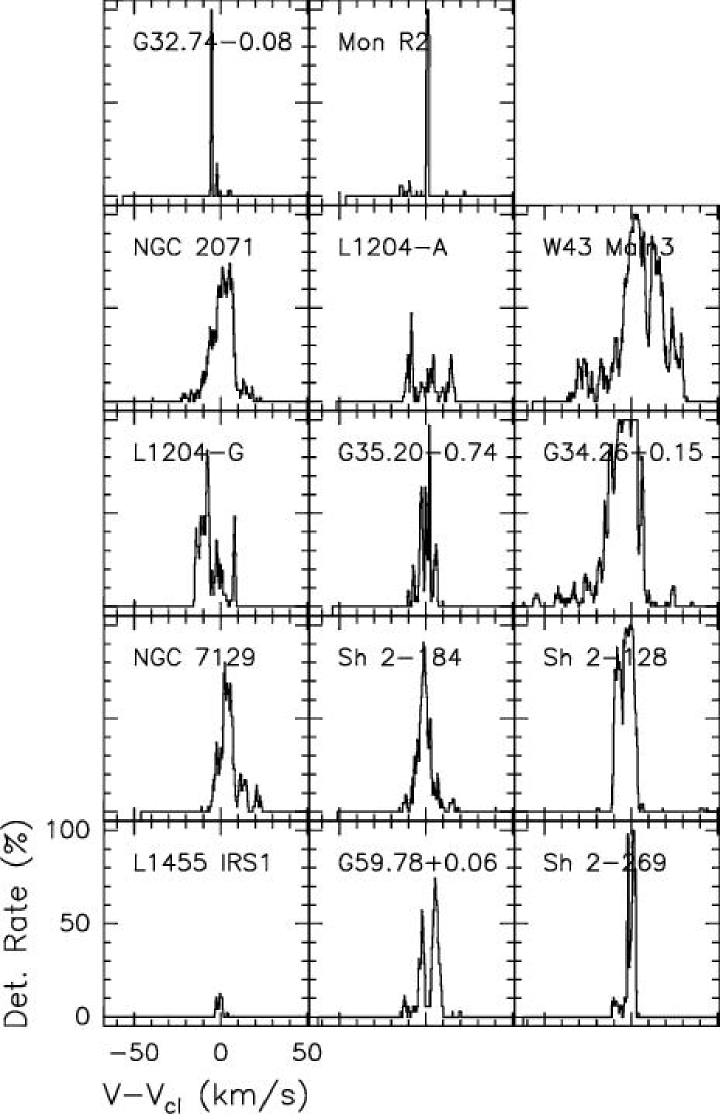
Figure 14: Frequency-of-occurrence histograms for all sources. All velocities are relative to $V_{cl}$. The panels are ordered in $L_{\rm fir}$, which increases from bottom to top and from left to right.

2.8.4 The scaled frequency-of-occurrence histograms

In Fig. 14 we show the frequency-of-occurrence histograms in order of increasing FIR luminosity (ordered as in Fig. 11). The velocity scale is the same in all plots and the velocities are referred to $V_{\rm cl}$ (i.e. the quantity on the horizontal axis is $V_{\rm observed}-V_{\rm cl}$).

We see that for sources with $L_{\rm fir}$$>3\times 10^{4}$ L_⊙ the peak of the distribution is always at 100% (i.e. these masers are always detected, cf. the lower envelopes discussion in the previous subsection), and it is always at or very close to $V_{\rm cl}$. Note that this is in agreement with the findings of Wouterloot et al. (wou95 (1995)), who concluded that for log$L_{\rm fir}$$>10^{4.5}$ (i.e. $L_{\rm fir}$$>3.2\times 10^{4}$ L_⊙) the maser detection rate is virtually 100%. For sources with lower values of $L_{\rm fir}$ the maser is typically detected (at the $\geq 5\sigma$ level) about 75%-80% of the time. Once more the exception is L1455 IRS1, which has a detection rate at these levels of only about 10%. For these lower-$L_{\rm fir}$ sources the peak of the distribution of emission components can also be much further away from $V_{\rm cl}$ than what is found for the high-$L_{\rm fir}$ sources (see also Sect. 2.1).

The steep decline of the histograms with velocity has already been commented on in Sect. 2.7, as showing that the more blue- and red-shifted maser components have shorter lifetimes than the components nearer the systemic (i.e. molecular cloud) velocity.

Many of the histograms in Fig. 14 show a main peak, and a collection of smaller peaks (hereafter ‘the tail’) on one side, while on the other side the decline is steeper. It seems that for sources with $L_{\rm fir}$ $>3\times 10^{4}$ L_⊙ the tail is preferentially on the blue side of the main peak (at these $L_{\rm fir}$’s this is so for all 5 objects except Sh 2-128), while at lower $L_{\rm fir}$ the tail is either mostly on the red side (as in NGC7129/FIRS2, L1204-G, G32.74$-$0.08, Sh 2-184) or the histogram does not show these smaller peaks at all (as in the case of L1204-A, G35.20$-$0.74, L1455 IRS1).

Masers and outflows are closely correlated (see e.g. Felli et al. FPT92 (1992)), with maser components at the bow shocks produced by the outflows upon impact with the ambient medium. Maser amplification is maximum in the plane of shocks, where the gain path is longest (Elitzur et al. eli89 (1989)); for high-velocity blue-shifted components the plane of the shock should be perpendicular to the line-of-sight, and therefore the gain path is rather short. However, in the case that a well-collimated outflow is precisely aligned with the line-of-sight, the maser can amplify the background continuum (from the Hii-region), and the high-velocity blue-shifted components can become more intense. This might be the case for the tail in high-luminosity sources. The collimation of the outflow, the alignment of the flow with the line-of-sight, and the Hii-region background radio continuum (hence the $L_{\rm fir}$ of the YSO) will determine the strength and the velocity offset (with respect to the molecular cloud velocity) of the high-velocity blue-shifted maser components. It appears that for the sources in our sample these three effects combine most favourably in G34.26$-$0.15 and W43 Main3 (with blue-shifted maser components up to $\sim 60$ km s^-1 and $\sim 40$ km s^-1 from $V_{\rm cl}$, respectively). According to this scenario the outflow in S 2-128 would not be aligned with the line-of-sight, or it could have a large opening angle (or both). The high-velocity red-shifted components (belonging to the part of the outflow moving away from us) will always be weaker, because they cannot amplify the continuum background. If there is no outflow, or if it is driven by a lower-luminosity YSO, high-velocity components (blue- or red-shifted) will not be seen at all. If the maser emission comes primarily from a protostellar disk, blue- and red-shifted components can be seen, but at velocities close to $V_{\rm cl}$.

The maser emission would therefore not only be a function of the luminosity of the exciting source, but also of the geometry of the SFR, in particular the orientation of the beam of the outflow.

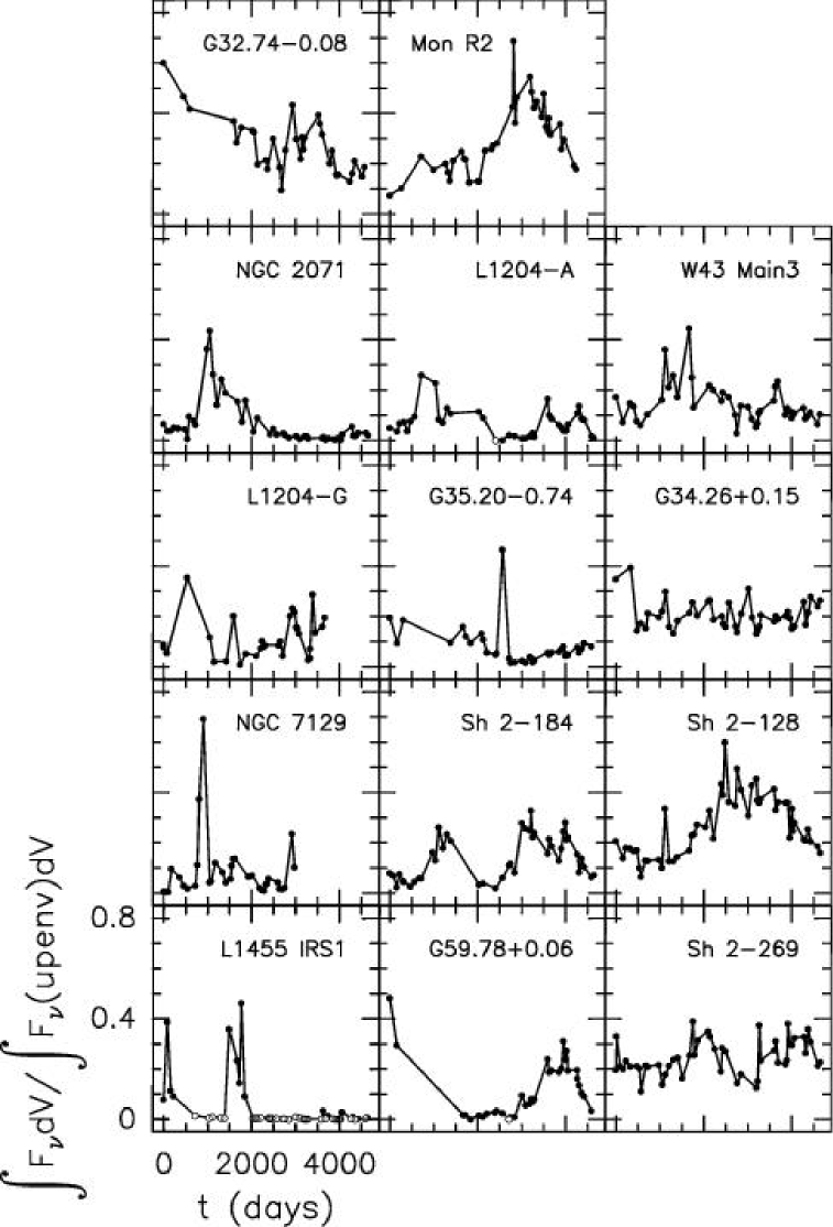
Figure 15: The integrated flux density, normalized by that of the upper envelope for each source. The panels are arranged by increasing $L_{\rm fir}$, which increases from bottom to top and from left to right. Open circles indicate non-detections.

2.8.5 The scaled integrated light-curves

In Fig. 15 we show the light curves of the integrated flux density $\int F{\rm d}V$ in order of increasing FIR luminosity, as in Fig. 11. The intensity for each source has been normalized to the integrated flux density of the upper envelope for that source.

The main phenomenon that emerges from these panels is that of global long-term (‘super’) variability, which was mentioned in Sect. 2.7: in addition to the occasional outbursts in total integrated flux density (sometimes due to a single maser component in a flaring stage), several of the sources appear to have a more gentle, long-term variability of the total maser output. This is most clearly seen in Sh 2-269 IRS2 and Sh 2-184, both of which show cyclic variations. The integrated emission of L1204-A is more fragmented and changes more erratically, yet also here we can see a hint of a general systematic variation of the total maser output with time. For G59.78+0.06 the first 2000 days are very poorly sampled, and it is therefore impossible to say if the broad peak we see near day 4000 has been preceded by a similar one during that earlier period. Mon R2 IRS3, Sh 2-128, and W43 Main3 may all show signs of global long-term variability as well, but with a period of the order of, or larger than, our monitoring period. The peak in NGC2071 on the other hand, might just be an outburst with a rapid increase in integrated flux density followed by a slow decline. We estimate that in Sh 2-184 a full cycle is completed in about 2000 days (5.5 yrs); the same is found for Sh 2-269 IRS2, which agrees with the $5.7\pm 1.0$ yr derived by Lekht et al. (lekht269 (2001)). Sh 2-128 has a cycle about twice as long (see also Lekht et al. lekht128 (2002)). A rough estimate for the period in L1204-A is $\approx 3000$ days (8.2 yrs). The origin of this long-term cyclic variation is not known, but in the hypothesis that H₂O masers are excited behind shocks caused by the impact of wind-driven outflows with the ambient medium, it seems natural to assume that the variation in the total maser output is either caused by a periodic variation in the YSO-wind or, for sources with non-periodic variation, by the turbulent motions in the material of the surrounding molecular cloud.

3 Summary

We have used the data collected during more than 10 years of monitoring H₂O masers in 14 SFRs (Valdettaro et al. paper1 (2001)), in order to extract general properties of the maser emission, and to investigate possible correlations between the various parameters of the maser emission (such as mean velocity, velocity extent, luminosity) and the FIR luminosity of the (presumable) driving source – usually an IRAS source. We have looked at velocity gradients of individual maser components, at the properties of bursts (their duration and their increase in flux density), and at long-term variations in the maser output.

One property that comes out clearly from this analysis is the existence of a general dependence of maser parameters on $L_{\rm fir}$. In addition there are indications of the existence of different $L_{\rm fir}$ regimes and a threshold YSO-luminosity that can account for the various observed characteristics of the H₂O maser emission. We find differences in some properties of the emission of masers associated with YSOs above and below a threshold luminosity of around $10^{4}$ L_⊙. Only for sources with $L_{\rm fir}$$\;\lower 2.58334pt\hbox{$\sim$}\kern-7.75pt\raise 2.79857pt\hbox{$>$}\;L_{\rm fir}^{\rm limit}$ a water maser is always detected. Above $L_{\rm fir}^{\rm limit}$ one finds increasingly morphologically complex maser emission, from the narrow, single emission component in Mon R2 to the broad, multi-component jungle of W43 Main3.

The main findings of this general analysis are summarized below.

1. The intensity-weighted mean velocity of the maser emission ($V_{\rm up}$) is close to that of the parental the molecular cloud ($V_{\rm cl}$); their difference, normalized to the total width ($\Delta V_{\rm up}$) of the maser emission is smaller if $L_{\rm fir}$(YSO) $\;\lower 2.58334pt\hbox{$\sim$}\kern-7.75pt\raise 2.79857pt\hbox{$>$}\;L_{\rm fir}^{\rm limit}\;\lower 2.58334pt\hbox{$\sim$}\kern-7.75pt\raise 2.79857pt\hbox{$>$}\;7\times 10^{3}$ L_⊙ (Sect. 2.1);

2. The velocity at which the maser emission is most intense, is also the velocity where emission occurs most frequently (Sect. 2.1);

3. $L_{\rm H_{2}O}^{\rm up}$, the luminosity the H₂O maser would have if all velocity components were to emit at their maximum level at the same time, is correlated with the YSO FIR luminosity $L_{\rm fir}$ by $L_{\rm H_{2}O}^{\rm up}$$=6.37\times 10^{-8}L_{\rm fir}^{0.81\pm 0.07}$ (Sect. 2.2);

4. The ratio between $L_{\rm H_{2}O}^{\rm max}$, the maximum H₂O luminosity measured during the entire monitoring period, and $L_{\rm H_{2}O}^{\rm up}$ ranges between 0.25 (Sh 2-269 IRS2) and 0.80 (Mon R2 IRS3), but does not depend on $L_{\rm fir}$ (Sect. 2.2);

5. The anti-correlation between $L_{\rm fir}$ and the ratio of the maximum and the mean integrated flux density indicates that high-luminosity sources tend to be associated with more stable masers, while lower luminosity ones have more variable emission (Sect. 2.3);

6. Higher maser power goes into more emission channels that are spread over a larger range in velocity. While in a diagram of $\Delta V_{\rm up}$ versus $L_{\rm fir}$ only an upper envelope can be defined, there is a real correlation between both the number of components and the maximum velocity extent of the maser emission and the luminosity of the H₂O maser if all are derived from the same spectrum (Sects. 2.4, 2.5);

7. For $\sim 15$ relatively isolated maser components we have made an analysis (using Gaussian-fits) of the emission velocity. We find both acceleration and deceleration in equal numbers, with gradients that range between 0.02 and 1.8 km s^-1 yr^-1. The smaller value refers to a component that could be traced over the whole 4600 days of monitoring; the higher value was found for a burst-component of $\sim 60$ day duration (Sect. 2.6);

8. We have looked in some detail at 14 outbursts in 9 emission components in 6 sources. The shortest/longest duration is $\sim 60/900$ days. Bursts of shorter duration are not detectable due to our sampling interval (typically 2-3 months), while those of longer duration are usually not recognized as a burst. The increase in flux density during a burst ranged from 40% to $\;\lower 2.58334pt\hbox{$\sim$}\kern-7.75pt\raise 2.79857pt\hbox{$>$}\;1840$%; the largest absolute increase was found in Mon R2 ($\sim 820$ Jy) (Sect. 2.7);

9. In several sources we find a complete (Sh 2-269 IRS2 and Sh 2-184) or partial (Mon R2 IRS3, Sh 2-128, and W43 Main3) cycle of integrated flux density changes over long timescales. For the first two sources we find this period to be of the order of 5.5 yrs. Also L1204-A may show such a long-term variation; in this case a rough estimate indicates a period of $\sim 8$ yrs (Sect. 2.8.5);

10. From the velocity-time-intensity plots we identify a limiting $L_{\rm fir}$ of $\sim 3\times 10^{4}$ L_⊙. For sources with $L_{\rm fir}$ above this limit the maser emission becomes increasingly structured and more extended in velocity with increasing $L_{\rm fir}$. Below this limit the maser emission shows the same variety of morphologies, but without a clear dependence on $L_{\rm fir}$ (Sect. 2.8.1);

11. From the lower envelopes we can identify the same limiting value of $L_{\rm fir}$$\approx 3\times 10^{4}$ L_⊙: all sources above this limit have at least one maser component that is always present, at a level of $1-20$% of the peak flux density in the upper envelope spectrum, and with a velocity very close to that of the upper envelope peak and to the molecular cloud velocity (Sect. 2.8.3);

12. From the upper envelopes we deduce the possible existence of three regimes of maser excitation, associated with three ranges in YSO $L_{\rm fir}$. For the lowest ranges, $L_{\rm fir}$$<4\times 10^{2}$ L_⊙ and $4\times 10^{2}$ L_⊙ $\sim$$<$  $L_{\rm fir}$$\;\lower 2.58334pt\hbox{$\sim$}\kern-7.75pt\raise 2.79857pt\hbox{$<$}\;6\times 10^{4}$ L_⊙, the maser excitation depends mostly on the strength of the outflow and the density of the surrounding molecular cloud, while for $L_{\rm fir}$$\;\lower 2.58334pt\hbox{$\sim$}\kern-7.75pt\raise 2.79857pt\hbox{$>$}\;6\times 10^{4}$ L_⊙ the YSO-luminosity is the determining factor (Sect. 2.8.3);

13. The frequency-of-occurrence histograms show that $L_{\rm fir}$ $\approx 3\times 10^{4}$ L_⊙ is a threshold value for the FIR luminosity of the presumed maser driving-source. For sources with $L_{\rm fir}$ above this limit the peak of the distribution is always at 100% (i.e. the maser is always detected). Below it, the typical detection rate (at the $>5\sigma$-level) $75-80$%. The exception is L1455 IRS1, which has a detection rate of only $\sim 10$% (Sect. 2.8.3). There is also a lower bound to $L_{\rm fir}$ (at least $\;\lower 2.58334pt\hbox{$\sim$}\kern-7.75pt\raise 2.79857pt\hbox{$<$}\;430$ L_⊙), below which the associated maser source is not detectable most of the time (Sect. 2.8.1).

14. The presence or absence of blue-shifted high-velocity maser components in the frequency-of-occurrence histograms led us to conclude that the maser emission is a function of not only the luminosity of the YSO, but also of the beaming properties of the outflow with respect to the observer (Sect. 2.8.4).

- (1) Anglada, G., Estalella, R., Pastor, J., Rodriguez, L.F., & Hascick, A.D. 1996, ApJ, 463, 205
- (2) Cesaroni R. 1990, A&A 233, 513
- (3) Claussen M.J., Wilking B.A., Benson P.J. et al. 1996, ApJS, 106, 111
- (4) Elitzur M. 1992, ARA&A 30, 75
- (5) Elitzur M., Hollenbach D.J., & McKee C.F. 1989, ApJ 346, 983
- (6) Elitzur M., Hollenbach D.J., & McKee C.F. 1992, ApJ 394, 221
- (7) Felli M., Palagi F., & Tofani G. 1992, A&A, 255, 293
- (8) Furuya R.S., Kitamura Y., Wootten A., Claussen M.J., & Kawabe R. 2001, ApJ 559, L143
- (9) Furuya R.S., Kitamura Y., Wootten A., Claussen M.J., & Kawabe R. 2003, ApJS 144, 71
- (10) Hunter T.R., Taylor G.B., Felli M., & Tofani G. 1994, A&A, 284, 215
- (11) Lada C.J. 1985, ARA&A 23, 267
- (12) Lekht E.E., Likhachev S.F., Sorochenko R.L., & Strel’nitskii V.S. 1993, Astron. Rep. 37, 367
- (13) Lekht E.E., Mendoza-Torres J.E., & Berulis I.I. 2002, Astron. Rep. 46, 57
- (14) Lekht E.E., Pashchenko M.I., & Berulis I.I. 2001, Astron. Rep. 45, 949
- (15) Liljeström, T., & Gwinn, C.R. 2000, ApJ, 534, 781
- (16) Palagi F., Cesaroni R., Comoretto G., Felli M., & Natale V. 1993, A&AS, 101, 153
- (17) Seth A.C., Greenhill L.J., & Holder B.P. 2002, ApJ 581, 325
- (18) Valdettaro R., Palla F., Brand J. et al. 2001, A&A, 383, 244 (Paper I)
- (19) Wilking B.A., Claussen M.J., Benson P.J. et al. 1994, ApJ 431, L119
- (20) Wouterloot J.G.A., Fiegle, K., Brand J., & Winnewisser, G. 1995, A&A, 301, 236 (Erratum: 1997, A&A 319, 360)