Separation of foreground and background signals in single frequency measurements of the CMB Polarization

Abstract

The polarization of the Cosmic Microwave Background (CMB)is a powerful observational tool at hand for modern cosmology. It allows to break the degeneracy of fundamental cosmological parameters one cannot obtain using only anisotropy data and provides new insight into conditions existing in the very early Universe. Many experiments are now in progress whose aim is detecting anisotropy and polarization of the CMB. Measurements of the CMB polarization are however hampered by the presence of polarized foregrounds, above all the synchrotron emission of our Galaxy, whose importance increases as frequency decreases and dominates the polarized diffuse radiation at frequencies below $\simeq 50$ GHz. In the past the separation of CMB and synchrotron was made combining observations of the same area of sky at different frequencies. In this paper we show that the statistical properties of the polarized components of the synchrotron and dust foregrounds are different from the statistical properties of the polarized component of the CMB, therefore one can build a statistical estimator which allows to extract the polarized component of the CMB from single frequency data also when the polarized CMB signal is just a fraction of the total polarized signal. Our estimator improves the signal/noise ratio for the polarized component of the CMB and reduces from $\simeq$50 GHz to $\simeq$20 GHz the frequency above which the polarized component of the CMB can be extracted from single frequency maps of the diffuse radiation.

, ,

1 Introduction

Almost a decade elapsed since the first detection of the anisotropy of the Cosmic Microwave Background at large angular scales ($\geq 10^{0}$) [Strukov et al. 92], [Smoot et al. 92]. Today the CMB anisotropy (CMBA) has been detected also at intermediate ($\sim(1^{0}-10^{0})$) and small angular scales ($\leq 1^{0}$), so the CMBA angular spectrum is now reasonably known down to the region of the  first  and  second  Doppler  peaks  [de Bernardis et al. 00],  [de Bernardis et al. 02], [Netterfield et al. 02]. Its shape gives information e.g. on the spectrum of the primordial cosmological perturbations or can be used to test the inflation theory but rises new questions to which CMBA cannot answers. It is however possible to get answers looking  at  the  CMB  polarization  (CMBP). For instance one can use CMBP to disentangle the effects of fundamental cosmological parameters like density of matter, density of dark energy etc. This is among the goals of space and ground based experiments like [MAP 03], [Delabrouille and Kaplan 02],  [Villa et al. 02],  [Kesteven 02],  [Piccirillo et al. 02], [Gervasi et al. 02], [Masi et al. 02] and is the main goal of SPOrt a polarization dedicated ASI/ESA space mission on the International Space Station [Cortiglioni et al. 99].

The relevance of the CMB polarization was remarked for the first time by M. Rees [Reees 68]. Since his paper many models of the expected features of the CMBP have been published (see for instance [Sazhin 95], [Ng and Ng 96], [Melchiorri and Vittorio 97]).  They  immediately  stimulated  the  search  for CMBP, but the first detection has been obtained only a few months ago ([Kovac et al. 02] and [Kogut et al. 03]). Because of its importance this discovery must be confirmed by new observations made with different systems and using different methods of extraction of the CMBP from the sky signal. The detection of the CMBP is in fact extremely difficult because the signal is at least an order of magnitude below the CMBA level. Moreover polarized foregrounds of galactic origin may cover the CMBP and/or mimic CMBP spots by their inhomogeneities. The signal to noise (CMBP $/$ polarized foreground) ratio is therefore $<<1$. In this paper we discuss a method which improves this ratio and allows to disentangle CMBP and polarized foregrounds.

In the microwave range the galactic foregrounds include:

• synchrotron radiation (strong polarization),

• free-free emission (null or negligible polarization),

• dust radiation (polarization possible)

Beccause here we are interested in polarization, in the following we will neglect free-free emission.The effects of dust, if present, (e.g. [Prunet et al. 98], [Fosalba et al. 02]), will be added to the synchrotron effects. In fact, as it will appears in the following, what matters in our analysis are the statistical properties of the spatial distribution of the foregrounds and, by good fortune, the spatial distribution of the dust polarized emission is similar to that of the synchrotron emission. Behind both types of radiation there is in fact the same driving force, the galactic magnetic field which alignes dust grains and guides the radiating electrons ([Bernardi et al. 03] and references therein).

For the anisotropy the separation of foregrounds and CMB  was  successfully solved  by  the DMR/COBE  team  when  they  discovered   CMBA [Smoot et al. 92]. The separation of CMBP and foregrounds is more  demanding  and recognizing true CMB spots among foreground inhomogneities severe.  Approaches   commonly   used ( e.g.  [Dodelson 97],   [Tegmark 99],     [Stolyarov et al. 02],    [Tegmark et al. 96],    [Kogut and Hinshaw 00],
 [Bennet et al. 03]), are based on the differences between the frequency spectra of foregrounds and CMB, therefore require multifrequency observations.

In this paper we suggest a different method. It takes advantage of the fact that, as we will show in the following, at small angular scales the values of the parameters used to describes the polarization of the diffuse radiation at a given frequency in different directions fluctuate. We propose of analyzing the angular distribution of the polarized radiation on single frequency maps of the diffuse radiation and disentangling the main components, polarized synchrotron and CMBP, looking to their different statistical properties. This method was proposed and briefly discussed in [Sazhin 02]. Here we present a more complete analysis.

2 Polarization Parameters

2.1 The Stokes Parameters

Convenient  quantities   commonly   used   to   describe  the   polarization  status   of   radiation   are the Stokes parameters   (see  for  instance
 [Ginzburg and Syrovatskii 65],  [Gardner and Whiteoak 66],
 [Ginzburg and Sirovatskii 69]).

Let’s assume a monochromatic plane wave of intensity I and amplitude $\propto\sqrt{I}$. In the observer plane, orthogonal to the direction of propagation of the electromagnetic wave, we can choose a pair of orthogonal axes ${\vec{l}}$ and ${\vec{r}}$. On that plane the amplitude vector of an unpolarized wave moves in a random way. On the contrary it describes a figure, the polarization ellipse, when the wave is polarized.

Projecting the wave amplitude on ${\vec{l}}$ and ${\vec{r}}$ we get two orthogonal, linearly polarized, waves of intensity $I_{l}$ and $I_{r}$,($I=I_{l}+I_{r}$) whose amplitudes are $\propto\sqrt{I_{l}}$ and $\propto\sqrt{I_{r}}$ respectively. If the original wave of intensity $I$ is polarized, $I_{l}$ and $I_{r}$ are correlated: let‘s call $I_{12}$ and $I_{21}$ their correlation products.

By definition the Stokes parameters are: $I=I_{l}+I_{r}$, $Q=I_{l}-I_{r}$, $U=I_{12}+I_{21}$, and $V=i(I_{21}-I_{12})$.

$Q$ and $U$ describe the linear polarization, $V$ the circular polarization and $I$ the total intensity.

The ratio

$$\tan 2\chi=\frac{U}{Q}$$ (1)

gives the angle $\chi$ between the vector $\vec{l}$ and the main axis of the polarization ellipse ($0<\chi<\pi$).

Rotation by an angle $\phi$ of the $(l,r)$ coordinate system give a new coordinate system $(\hat{l},\hat{r})$ in which the Stokes parameters become

$$\begin{array}[]{c}\hat{Q}=Q\cos 2\phi-U\sin 2\phi\\ {}\hfil\\ \hat{U}=U\cos 2\phi+Q\sin 2\phi\end{array}$$ (2)

So when $\phi=\chi=(1/2)\arctan{\frac{U}{Q}}$ the axes of the polarization ellipse coincide with the reference axes $\hat{l}$ and $\hat{r}$ (see fig.1).

         

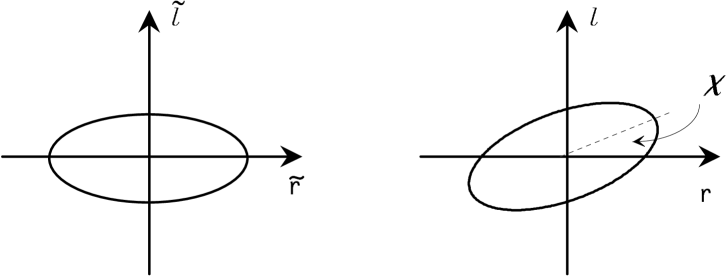
Figure 1: The polarization ellipse

2.2 Electric and Magnetic Modes

To analyze the properties of the CMB polarization it is sometimes convenient to use rotationally invariant quantities, like the radiation intensity $I$ and two combinations of $U$ and $Q$: $Q+iU$ and $Q-iU$. The intensity $I$ can be decomposed into usual (scalar) spherical harmonics $Y_{lm}(\theta,\varphi)$.

$$I=\sum_{l,m}a_{lm}Y_{lm}(\theta,\varphi)$$ (3)

The quantities $Q\pm iU$  can  be   decomposed  into   $\pm 2$  spin harmonics
[Sazhin et al. 96a],   [Sazhin et al. 96b],   [Seljak and Zaldarriaga 97]
$Y_{lm}^{\pm 2}(\theta,\varphi)$ :

$$Q\pm iU=\sum_{l,m}a_{lm}^{\pm 2}Y_{lm}^{\pm 2}(\theta,\varphi)$$ (4)

The $\pm 2$ spin harmonics form a complete orthonormal system (see, for instance, [Goldberg et al. 67],[Gelfand et al. 58], [Zerilli 70], [Thorn 80]) and can be written [Sazhin et al. 96b], [Sazhin and Sironi 99]:

$$\begin{array}[]{c}Y^{2}_{lm}(\theta,\varphi)=N^{2}_{lm}P^{2}_{lm}(\theta)e^{im\varphi}\\ {}\hfil\\ Y^{-2}_{lm}(\theta,\varphi)=N^{-2}_{lm}P^{-2}_{lm}(\theta)e^{im\varphi}\end{array}$$ (5)

where

$$P^{s}_{lm}(x)=(1-x)^{\displaystyle(m+s)\over 2}(1+x)^{\displaystyle(s-m)\over 2}P^{(m+s,s-m)}_{l-s}(x)$$ (6)

is a generalized Jacobi polynomial, $s=\pm 2$ and:

$$N^{s}_{lm}=\frac{1}{2^{s}}\sqrt{\frac{2l+1}{4\pi}}\sqrt{\frac{(l-s)!(l+s)!}{(l-m)!(l+m)!}}$$

is a normalization factor.

The harmonics amplitudes $a^{\pm 2}_{lm}$ correspond to the Fourier spectrum of the angular decomposition of rotationally invariant combinations of Stokes parameters.

Because spin $\pm 2$ spherical functions form a complete orthonormal system:

$$\int_{4\pi}Y^{\pm 2}_{lm}(\theta,\varphi)Y^{*\;\pm 2}_{l^{\prime}m^{\prime}}(\theta,\varphi)d\Omega=\delta_{lm}\delta_{l^{\prime}m^{\prime}}$$ (7)

we can write

$$a^{\pm 2}_{lm}=\int_{4\pi}d\Omega\;\;\left(Q(\theta,\varphi)\pm iU(\theta,\varphi)\right)Y^{*\;\pm 2}_{lm}$$ (8)

Following [Seljak and Zaldarriaga 97] and the very nice introduction made more recently by [Zaldarriaga 01] we now introduce the so called $E$ (electric) and $B$ (magnetic) modes of these harmonic quantities:

$$\begin{array}[]{c}a^{E}_{lm}=\frac{1}{2}\left(a^{+2}_{lm}+a^{-2}_{lm}\right)\\ {}\hfil\\ a^{B}_{lm}=\frac{i}{2}\left(a^{+2}_{lm}-a^{-2}_{lm}\right)\end{array}$$ (9)

They have different parities. In fact when we transform the coordinate system $Oxyz$ into a new coordinate system $\tilde{O}\tilde{x}\tilde{y}\tilde{z}$, such that

$$\begin{array}[]{c}\tilde{\vec{l}}=\vec{l}\\ \tilde{\vec{r}}=-\vec{r}\end{array}$$ (10)

the E and B modes transform in a similar way:

$$\begin{array}[]{c}\tilde{a}^{E}=a^{E}\\ \tilde{a}^{B}=-a^{B}\end{array}$$ (11)

$Q$ remains identical in both reference systems and $U$ changes sign.

It is important to remark that $a^{E}$ and $a^{B}$ are uncorrelated.

In terms of $Q$ and $U$ we can write:

$$\begin{array}[]{c}a^{E}_{lm}=\frac{1}{2}\int d\Omega\;\;\left(Q\left(Y^{+2}_{lm}+Y^{-2}_{lm}\right)+iU\left(Y^{+2}_{lm}-Y^{-2}_{lm}\right)\right)\\ {}\hfil\\ a^{B}_{lm}=\frac{1}{2}\int d\Omega\;\;\left(iQ\left(Y^{+2}_{lm}-Y^{-2}_{lm}\right)-U\left(Y^{+2}_{lm}+Y^{-2}_{lm}\right)\right)\end{array}$$ (12)

therefore :

$$\begin{array}[]{c}\left<(a^{E}_{lm})^{2}\right>-\left<(a^{B}_{lm})^{2}\right>=\\ ~{}~{}~{}~{}~{}=~{}2\int d\Omega\left(\left<|Q^{2}|\right>-\left<|U^{2}|\right>\right)\left(Y^{+2}_{lm}Y^{*-2}_{lm}+Y^{*+2}_{lm}Y^{-2}_{lm}\right)\end{array}$$ (13)

Here $\left<|Q^{2}|\right>$ and $\left<|U^{2}|\right>$ designate values of delta correlated 2D stochastic fields $Q$ and $U$. Omitting mathematical details, the correlation equations for $Q$ and $U$ are:

$$\begin{array}[]{c}\left<QQ^{*}\right>=|Q^{2}|\delta(\Omega-\Omega^{\prime})\\ {}\hfil\\ \left<UU^{*}\right>=|U^{2}|\delta(\Omega-\Omega^{\prime})\\ {}\hfil\\ \left<QU^{*}\right>=0\end{array}$$ (14)

where $\delta(\Omega-\Omega^{\prime})=\delta(\cos\theta-\cos\theta^{\prime})\cdot\delta(\varphi-\varphi^{\prime})$ is the Dirac delta - function on the sphere. (In the following we will sometimes omit indexes $l$ and $m$).

3 Synchrotron Radiation and its Polarization

Synchrotron radiation results from the helical motion of extremely relativistic electrons around the field lines of the galactic magnetic field (see, for instance [Ginzburg and Syrovatskii 65], [Ginzburg and Sirovatskii 69], [Westfold 59]). The electron angular velocity

$$\omega_{e}=\frac{eH_{p}}{m_{e}c}~{}\frac{m_{e}c^{2}}{\mathcal{E}}=\omega_{o}\frac{m_{e}c^{2}}{\mathcal{E}}$$ (15)

is determined by the ratio between $H_{p}$, the component of the magnetic field orthogonal to the particle velocity, and $\mathcal{E}$, the electron energy. As it moves around the magnetic field lines the electron radiates.

a)Single electron

Until the electron velocity is small ($v<<c$) we speak of cyclotron radiation: the electron behaves as a rigid dipole which rotates with gyrofrequency (15) in a plane orthogonal to the magnetic field direction and emits a single line. The radiation has a dumbell spatial distribution (see fig.2):

$$I(\Theta,\Phi)\sim(1+\cos^{2}\Theta),$$ (16)

is circularly polarized along the dumbell axis ($\Theta=0$) and linearly polarized in directions orthogonal to it ($\Theta=90^{\circ}$).

         

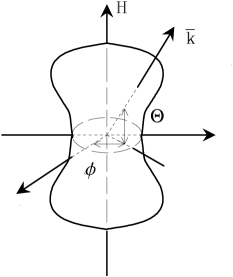
Figure 2: Spatial distribution of the cyclotron radiation produced by a single electron (see eq.16)

When the electron velocity increases the radiation field changes until at $v\approx c$, ($\mathcal{E}$ $\gg m_{e}c^{2}$) it assumes the peculiar charachters of synchrotron radiation:

i)radiated power proportional to $\mathcal{E}$ ² and $H_{p}^{2}$,

ii)continous frequency spectrum, peaked around:

$$\omega_{m}(\psi)=\omega_{o}\frac{\sqrt{1-\frac{v^{2}}{c^{2}}}}{1-\frac{v}{c}\cos\psi}~{}\propto H_{p}{\mathcal{E}}^{2}$$ (17)

($\psi$ is the angle between the velocity vector $\vec{v}$ and the wave vector $\vec{k}$, see fig.3). The peak is so narrow that in a given direction the emission is practically monochromatic,

         

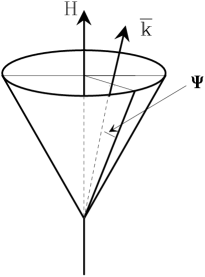
Figure 3: Velocity cone of an ultrarelativistic ($v\simeq c$) electron ($H$ = magnetic vector, $k$ wave vector, $\psi$ angle between the electron velocity and the direction of observation)

iii)radiation almost entirely emitted in a narrow cone of aperture (see fig.4)

$$\psi\approx\frac{m_{e}c^{2}}{\mathcal{E}}$$ (18)

around the forward direction of the electron motion. Inside the cone ($\cos\psi\approx 1$) the frequency is maximum and equal to

$$\omega_{m,o}\approx\omega_{o}\left(\frac{{\mathcal{E}}}{m_{e}c^{2}}\right)^{2},$$ (19)

In the opposite direction ($\cos\psi\approx-1$) intensity and frequency are sharply reduced.

         

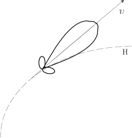
Figure 4: Distribution of the radiation emitted by an ultrarelativistic ($v\simeq c$) electron with istantaneous velocity $v$ spiralling (dashed line) around the lines of the magnetic field $H$ (orthogonal to the sheet)

iv)radiation 100 $\%$ linearly polarized at the surface of the cone.Inside the cone the linear polarization is still dominant but a small fraction of circular polarization exists, ($V\sim o(\frac{m_{e}c^{2}}{E})$ and $I\sim U\sim Q$). Outside the cone the very small fraction of radiation produced is elliptically polarized and becomes circularly polarized when seen along the $H_{p}$ direction. So the Stokes parameters depend on $H$, the angle $\mu$ between $H$ and the line of sight, and the dimensionless frequency $\nu/\nu_{c}$, where $\nu_{c}=1.5(\omega_{m}(0)/2\pi)$ is the so called critical frequency, [Ginzburg and Syrovatskii 65],[Ginzburg and Sirovatskii 69], itself function of $H$ (see eq.15).

b)Cloud of monoenergetic electrons

When the effects of many monoenergetic electrons with uniform distribution of pitch angles are combined, $I,Q$ and $U$ are reinforced (the Stokes parameters are additive) while $V$ is erased. In fact

$$\begin{array}[]{c}I(\nu)=c_{1}H_{p}F(\frac{\nu}{\nu_{c}})\\ {}\hfil\\ Q(\nu)=c_{2}H_{p}F_{p}(\frac{\nu}{\nu_{c}})\cos 2\chi\\ {}\hfil\\ U(\nu)=c_{2}H_{p}F_{p}(\frac{\nu}{\nu_{c}})\sin 2\chi\\ {}\hfil\\ V(\nu)\approx 0\end{array}$$ (20)

where $c_{1}$ and $c_{2}$ are constants, $F$ and $F_{p}$ almost monochromatic functions of $\nu$ , and $\chi$ the angle between the projection of the magnetic vector on the observer plane and an axis on that plane (The projection of the magnetic vector on the observer plane is the minor axis of the polarization ellipse). If inside the emitting cloud the magnetic field varies, also $\chi$ varies, therefore $\cos 2\chi$ and $\sin 2\chi$ must be averaged along the line of sight across the cloud. In conclusion the degree of polarization $p$ varies between a maximum value, (uniform magnetic field) and zero (magnetic field randomly distributed).

c)Electrons with power law energy spectrum

In the interstellar medium the radiating particles are the cosmic ray electrons whose energy spectrum :

$$N(\mathcal{E})=K\mathcal{E}^{-\gamma}$$ (21)

is a power law (see for instance [Gavazzi and Sironi 75], [Longair 94]) and references therein) with spectral index $\gamma\approx 2.4-3.0$ and space density proportional to $K$. Because the emission of a single electron is practically monochromatic the resulting radiation spectrum is a power law:

$$I(\nu)=I_{0}(\gamma)H_{p}^{\frac{\gamma+1}{2}}\nu^{-\beta^{\prime}}$$ (22)

with intensity spectral index $\beta^{\prime}=\frac{\gamma-1}{2}$, temperature spectral index $\beta=\beta^{\prime}+2$ and $I_{0}$ a slow function of $\gamma$ [Ginzburg and Syrovatskii 65]. (If the magnetic field is not uniform we use $<H_{p}>$ instead of $H_{p}$ and a slightly different function $I_{0}(\gamma)$).

The Stokes parameters are products of the intensity $I(\nu)$, the degree of polarization $p$ and $\cos 2\chi$ or $\sin 2\chi$, therefore we can write:

$$\begin{array}[]{c}Q=c_{3}~{}H_{p}^{\frac{\gamma+1}{2}}~{}\nu^{-\frac{\gamma-1}{2}}\cos 2\chi\\ {}\hfil\\ U=c_{3}~{}H_{p}^{\frac{\gamma+1}{2}}~{}\nu^{-\frac{\gamma-1}{2}}\sin 2\chi\\ {}\hfil\\ V\approx 0\end{array}$$ (23)

where $c_{3}$ is a constant whose value depends on $\gamma$ and the distribution of the magnetic field along the integration path.

When the medium inside the synchrotron source, or in the medium where radiation propagates, is permeated by thermal electrons Faraday rotation modifies the polarization charachteristics of the radiation. In fact by Faraday effect, when the radiation crosses a region of thickness $L$ permeated by magnetic fields and thermal electrons with density $n_{e}$, the angle of polarization of the radiation rotates by an angle (see for instance [Rybicki and Lightman 79])

$$\theta~{}=~{}cost~{}<n_{e}>~{}L~{}\lambda^{2}$$ (24)

Inside the source this brings depolarization, because radiation produced at different points along $L$ suffers different rotations. Additional depolarization inside the source comes about when the magnetic field along $L$ is not uniform because in eqs.(23)we have to use $<\sin 2\chi>$ and $<\cos 2\chi>$ instead of $\sin 2\chi$ and $\cos 2\chi$. So the degree of polarization at the source $p$ varies between 0 (random magnetic field distribution) and:

$$p_{max}=\frac{3\gamma+3}{3\gamma+7}<1$$ (25)

(uniform magnetic field and Faraday rotation absent).

Outside the source the angle of polarization rotates by Farday effect so the Stokes Parameter of the synchrotron radiation $Q_{s}$ and $U_{s}$ measaured by an Earth observer are different from the Stokes Parameters at the source.

A regular trend of the magnetic field inside and outside the source is insufficient to guarantee a regular trend of the spatial distribution of $Q_{s}$ and $U_{s}$. In fact as the line of sight moves among adjacent points on the sky $n_{e}$, $<n_{e}>$ and $L$ fluctuate. So also the angle of Faraday rotation $\theta$ fluctuates by a quantity

$$\begin{array}[]{c}\delta\theta~{}=~{}cost~{}\lambda^{2}~{}\delta(<n_{e}>L){}{}{}{}{}{}{}{}{}{}{}{}{}{}{}{}{}{}{}{}{}{}{}{}{}{}{}{}{}{}{}{}{}{}{}{}{}{}{}{}{}\\ \\ \simeq~{}cost~{}\lambda^{2}~{}\{[L~{}\delta(<n_{e}>)]^{2}~{}+~{}[<N_{e}>\delta(L)]^{2}\}^{1/2}~{}\simeq~{}cost~{}\lambda^{2}~{}L~{}\delta(n_{e})\end{array}$$ (26)

proportional to $L$. Because L is at least tens or hundred of pc $\delta\theta$ can be very large. Besides this effect produced by Faraday rotation, when we look in different directions through the interstellar medium $Q_{s}$ and $U_{s}$ may change also because $H$, $H_{p}=H\sin\mu$, $\gamma$, $\beta$ and $K$ vary (see for instance [Wielebinski 02], [Reich et al. 02]) .

We conclude that angle and degree of polarization of the synchrotron radiation fluctuates when the line of sight moves among adjacent regions on the sky, a conclusion supported by recent observations which show that the spatial distribution of the polarized component of the synchrotron radiation at intermediate and small angular scales is highly structured. On maps we see in fact lines (channels) along which $p$ goes to zero and sudden rotations of the plane of polarization when the line of sight goes from a side to the other of a channel [Shukurov and Berkhuijsen 03].

We expect therefore that at small and intermediate angular scales $Q_{s}$ and $U_{s}$ are stochastic functions of the direction of observations so we can write:

$$\left<Q^{2}_{s}\right>=\left<U^{2}_{s}\right>$$ (27)

Exceptions to this behaviour can be expected when along the line of sight there are peculiar regions characterized by special field configurations and/or by large densities of thermal electrons, like in the well known loops and spurs or in HII regions, where systematic effects overcome random effects. Nature and origin of these features, clearly visible on Brouw and Spoelstra maps of the polarized component of the galactic background [Brouw and Spoelstra 76], are discussed for instance by [Salter and Brown 88]. Usually these regions are close to the observer and have large angular dimensions, so their effects can be removed if one evaluates the angular power spectrum of the radiation distribution and limits his analysis to angular scales below few degrees (multipole order $l>150$) .

Being aware that this is a very important issue we tested its validity analyzing the distribution of the measured values of $Q$ and $U$ on maps extracted from the Effelsberg survey ([MIPFR-Bonn 03] and [Duncan et al. 99]) of the diffuse radio emission. We found (see Appendix 2) that up to angular scales of 5 degrees (l close to 36) the difference $<Q^{2}>-<U^{2}>$ is fully consistent with zero.

Because of eq. (27) if $Q_{s}\neq 0$ also $U_{s}\neq 0$, so the synchrotron radiation has both electric and magnetic modes:

$$a^{E,s}\neq 0,\hskip 56.9055pta^{B,s}\neq 0$$ (28)

and (see eqs. (13) and (27)):

$$\left<(a^{E,s})^{2}\right>=\left<(a^{B,s})^{2}\right>$$ (29)

4 Stokes Parameters of the CMB

In a homogeneous and isotropic Universe only temperature and intensity $I=I_{l}+I_{r}$ change as the Universe expands : both decrease adiabatically. Because this is true for $I_{l}$ and $I_{r}$ separately, we do not expect anisotropy nor polarization therefore $Q=0$ and $U=I_{u}=0$ are natural consequences.

On the contrary, inhomogeneities and perturbations of matter density or of gravitational field, induce anisotropy and polarization of the CMB. At the recombination epoch linear polarization appears as a by product of the Thomson scattering of the CMB on the free electrons of the primordial plasma. The polarizarion tensor it gives can be calculated solving the Boltzman transfer equations of the radiation in a nonstationary plasma permeated by a variable and inhomogeneous gravitational field [Basko and Polnarev 80], [Sazhin 84], [Harrari and Zaldarriaga 93], [Sazhin 95].

The gravitational field is made of a background field, with homogeneous and isotropic FRW metric, and an inhomogeneous and variable mix of waves: density fluctuations, velocity fluctuations, and gravitational waves. Because of their transformation laws these waves are also said scalar, vector and tensor perturbations, respectively.

4.1 Scalar (density) perturbations

Scalar (density) perturbations affect the gravitational field, the density of matter and its velocity distribution. They were discovered studying the matter distribution in our Universe on scales from $\sim 1$ Mpc to $\sim 100$ Mpc. It is firmly believed they are the seeds of the large scale structure of the Universe and are reflected by the large scale CMB anisotropy detected for the first time at the beginning of the ‘90s [Strukov et al. 92], [Smoot et al. 92]. Their existence is predicted by the great majority of models of the early Universe.

Observation shows that the effects of these perturbations are small, so we can treat them as small variations $\delta_{l}$, $\delta_{r}$, $\delta_{u}$ of $I_{l}$, $I_{r}$ and $I_{u}$. Introducing the auxiliary functions $\alpha$ and $\beta$:

$$\begin{array}[]{c}\delta_{l}+\delta_{r}=(\mu^{2}-{1\over 3})\alpha,\\ {}\hfil\\ \delta_{l}-\delta_{r}=(1-\mu^{2})\beta,\\ {}\hfil\\ \delta_{u}=0,\end{array}$$ (30)

($\mu$ is the angle between the line of sight and the wave vector) for plane waves the Boltzman equations (see for instance [Sazhin 95], [Sazhin et al. 96a], [Sazhin et al. 96b] and reference therein) become:

$$\begin{array}[]{c}\frac{d\alpha}{d\eta}=F-\frac{9}{10}\sigma_{T}n_{e}a(\eta)\alpha-\frac{6}{10}\sigma_{T}n_{e}a(\eta)\beta\\ {}\hfil\\ \frac{d\beta}{d\eta}=-\frac{1}{10}\sigma_{T}n_{e}a(\eta)\alpha-\frac{4}{10}\sigma_{T}n_{e}a(\eta)\beta\end{array}$$ (31)

where $F$ is the gravitational force which drives both anisotropy and polarization, $\sigma_{T}$ is the Thomson cross-section, $n_{e}$ is the density of free electrons, and $a(\eta)$ the scale factor.

These equations give:

$$\begin{array}[]{c}Q=-\frac{1}{7}(1-\mu^{2})\int F(\eta)\left(e^{-\tau}-e^{-{3\over 10}\tau}\right)d\eta\\ {}\hfil\\ U=0\end{array}$$ (32)

where $\tau(\eta)$ is the optical depth of the region where the phenomenon occurs. Rotating the coordinate system we can generate a new pair of Stokes parameters ($Q^{\prime},U^{\prime}$): no matter which is the system of reference we choose these parameters satisfy the symmetry parity condition.

Because there is always a system in which $Q\neq 0$ and $U=0$, we may conclude that, in a system dominated by the primordial density perturbations (see, for instance [Dolgov et al. 90]) magnetic modes of the CMB polarization vanish and only electric modes exist [Seljak and Zaldarriaga 97]. Therefore:

$$a^{E,d}\neq 0\hskip 56.9055pta^{B,d}=0$$ (33)

where index $d$ stays for density perturbation.

4.2 Vector (velocity) perturbations

Vector perturbations, associated to rotational effects, perturb only velocity and gravitational field. They are not predicted by the inflation theory and it is common believe that they do not contribute to the anisotropy and polarization of the CMB.

4.3 Tensor (gravitational waves) perturbations

Gravitational waves (tensor modes) and gravitational lensing of large scale structures of the Universe induce B modes in the distribution of CMBP(see for instance [Hu et al. 03])) . Gravitational lensing gives a power spectrum at least an order of magnitude below the power spectrum of the E mode polarized signal produced by scalar perturbations, with a maximum at $l\simeq 1000)$. The power spectrum of the B mode polarization produced by gravity waves is maximun at $l\simeq 90$, is definitely below the power spectrum produced by gravitational lensing for $l>100$ and only at very large angular scales ($l\simeq 20$) it may be comparable to the scalar E modes.

If one excludes very large angular scales we may conclude that CMBP is dominated by E-modes. B-modes are just a contamination by B-modes at levels of $10\%$ or less.

5 Separation of the polarized components of Synchrotron and CMB Radiation

The CMB radiation we receive is mixed with foregrounds of local origin. When the anisotropy of the CMB was detected, to remove the foregrounds from maps of the diffuse radiation, data were reorganized in the following way:

$$\hat{T}_{d}(x,y)=\hat{T}_{n}(x,y)+\hat{M}_{i}(x,y)\hat{T}_{i,c}(x,y)$$ (34)

where $\hat{T}_{d}$, is a two dimension vector (map) which gives the total signal measured at different points $(x,y)$ on the sky, $\hat{T}_{n}$ the noise vector, $\hat{M}$ the matrix which combines the components $\hat{T}_{i,c}$ of the signal. At each point $(x,y)$ we can in fact write:

$$T_{d}=g_{n}T_{n}+g_{cmb}T_{cmb,c}+g_{syn}T_{syn,c}+g_{ff}T_{ff,c}+g_{dust}T_{dust,c}+...$$ (35)

where $g_{i}$ are weights, given by $M$, $T_{syn,c}$ is the synchrotron component, $T_{ff,c}$ the free-free emission component, $T_{dust,c}$ the dust contribution and so on. Using just one map the signal components cannot be disentangled. If however one has maps of the same region of sky made at different frequencies it is possible to write a system of equations. Provided the number of maps and equations is sufficient, the system can be solved and the components of $T_{d}$ separated, breaking the degeneracy. We end up with a map of $T_{cmb}$ which can be used to estimate the CMB anisotropy.

When we look for polarization at each point on the sky we measure tensors instead of scalar quantities, therefore to disentangle the polarized components of the CMB we need a greater number of equations. Here we will concentrate on the separation of the two dominant components of the polarized diffuse radiation: galactic synchrotron (plus dust) foreground and CMBP.

5.1 The estimator $D$

Instead of observing the same region of sky at many frequencies, we suggest a different approach. It takes advantage of the differences between the statistical properties of the two most important components of the polarized diffuse radiation (CMB (background) and synchrotron (foreground) radiation) and does not require multifrequency maps.

We define the estimator:

$$D=\left<(a^{E})^{2}\right>-\left<(a^{B})^{2}\right>$$ (36)

where $a^{E}=a^{E,s}+a^{E,c}$ and $a^{B}=a^{B,s}+a^{B,c}$ (here and in the following indexes $s$ or $c$ stay for synchrotron and CMB, respectively).

Because

• $E$ and $B$ modes of synchrotron do not correlate each other neither correlate with the CMB modes

  $\left<(a^{E})^{2}\right>=\left<(a^{E,s})^{2}\right>+\left<(a^{E,c})^{2}\right>+2\left<a^{E,s}a^{E,c}\right>=\left<(a^{E,s})^{2}\right>+\left<(a^{E,c})^{2}\right>$,

  $\left<(a^{B})^{2}\right>=\left<(a^{B,s})^{2}\right>+\left<(a^{B,c})^{2}\right>+2\left<a^{B,s}a^{B,c}\right>=\left<(a^{B,s})^{2}\right>+\left<(a^{B,c})^{2}\right>$,

• $~{}~{}~{}~{}~{}~{}~{}~{}~{}~{}~{}~{}~{}<a^{E,s}>=<a^{B,s}>\neq 0$

• $$a^{E,c}=a^{E,d}\neq 0\hskip 113.81102pta^{B,c}=a^{B,t}\leq 0.1~{}a^{E,d}$$

where indexes $d$ and $t$ stay for $density$ (or $scalar$) and $tensor$ perturbation, respectively.

$D$ gives an estimate of the E-mode excess in maps of the polarized diffuse radiation. If tensor perturbations are negligible this excess is the CMBP signal. If tensor perturbations are important the excess is a lower limit with a systematic difference from the true value which in the worst condition (maximum contribution to CMBP from gravitational waves and gravitational lensing) reaches a maximum value of $10\%$.

Let‘ s now consider the angular power spectrum of $D$. For multipole $l$ we can write:

$$D_{l}=(a^{E}_{l})^{2}-(a^{B}_{l})^{2}=\frac{1}{2l+1}\sum_{m=-l}^{l}\left(|a^{E}_{lm}|^{2}-|a^{B}_{lm}|^{2}\right)$$ (37)

where $|a^{E}_{lm}|^{2}$ and $|a^{B}_{lm}|^{2}$ are random variables with gaussian distribution $p(a_{lm}^{E,B})$ (see eqs.(56) and (57) in Appendix A). According the ergodic theorem (in the limit of infinite maps, the average over 2D space is equivalent to the average over realisations) the average value of $D_{l}$ is equal to the difference of the average values of $|a^{E}_{lm}|^{2}$ and $|a^{B}_{lm}|^{2}$ summed over $m$. Taking into account equation (57) we can therefore write:

$$\left<D_{l}\right>=\left(|a^{E}_{l}|^{2}-|a^{B}_{l}|^{2}\right)$$ (38)

where :

$$\begin{array}[]{c}(a^{E}_{l})^{2}=\int\limits^{\infty}_{-\infty}|a_{lm}^{E}|^{2}p(a_{lm}^{E})d^{2}a^{E}_{lm}=\left<|a_{lm}^{E}|^{2}\right>\\ {}\hfil\\ (a^{B}_{l})^{2}=\int\limits^{\infty}_{-\infty}|a_{lm}^{B}|^{2}p(a_{lm}^{B})d^{2}a^{B}_{lm}=\left<|a_{lm}^{B}|^{2}\right>\end{array}$$ (39)

Comparing eq.(39) with the ordinary definition of multipole coefficients:

$$C_{l}^{E,B}=\frac{1}{2l+1}\sum_{m=-l}^{l}\left<|a_{lm}^{E,B}|^{2}\right>$$ (40)

we can write:

$$\begin{array}[]{c}(a^{E}_{l})^{2}=C^{E}_{l}\\ {}\hfil\\ (a^{B}_{l})^{2}=C^{B}_{l}\end{array}$$ (41)

5.2 Separation uncertainty

For synchrotron radiation $\left<D_{l}\right>$ should be zero, non zero for density perturbations, but on real maps it is always different from zero. In fact a map is just a realization of a stochastic process and the amplitudes of $|a^{E}_{lm}|^{2}$ and $|a^{B}_{lm}|^{2}$, averaged over 2D sphere, have uncertainties which add quadratically, so $\left<D_{l}\right>\neq 0$ even in the case of synchrotron polarization. This effect, very similar to the well known cosmic variance of anisotropy [Knox and Turner 94], [Sazhin et al. 95] (the real Universe is just a realisation of a stochastic process, therefore there will be always a difference between the realization we measure and the expectation value) does not vanish if observations are repeated.

The variance of $D_{l}$ is

$${\bf V}(D_{l}^{2})=\left<D_{l}^{2}\right>-\left<D_{l}\right>^{2}$$ (42)

The quantities $a^{E}$ and $a^{B}$, being sums over $m$ of $2l+1$ stochastic values with gaussian distribution, have a $\chi^{2}$ distribution with $2*(2l+1)$ degrees of freedom, so their variance is

$$\delta(a^{E,B})^{2}\propto\sqrt{\frac{2}{2l+1}}$$ (43)

More explicitly

$$\left<D^{2}_{l}\right>=\frac{1}{2l+1}\left((a_{l}^{E})^{4}+(a_{l}^{B})^{4}\right)$$ (44)

When the synchrotron foreground is dominant ($a_{l}^{E}=a_{l}^{B}$)

$$\left<D^{2}_{l}\right>=\frac{2}{2l+1}(a^{E}_{l})^{4}$$ (45)

in agreement with (43).

5.3 A criterium for CMBP detection

The synchrotron foreground is a sort of system noise which hampers the detection of the signal, the CMB polarization. At frequencies sufficiently high (above $\sim 50$ GHz, see next section) the noise is small compared to the signal therefore direct detection of CMBP is possible. At low frequencies on the contrary the CMBP signal is buried in the noise created by synchrotron and dust emission. In this case to recognize the presence of the CMB polarization we can use our estimator $D$.

At angular scale $l$, to be detectable the CMBP must satisfy the condition

$$C_{l}^{E,c}>A\cdot C_{l}^{E,s}$$ (46)

where $C_{l}^{E,i}$ are the coefficients of the multipole expansion of the $E$ modes and $A$ is the confindence level of the signal detectability. In a similar way we can write for our estimator:

$$D_{l}^{E,c}>A\cdot D_{l}^{E,s}$$ (47)

where

$$D_{l}^{E,s}=\sqrt{\frac{2}{2l+1}}(a_{l}^{E,s})^{2}$$ (48)

If one neglects tensor perturbations ($D_{l}^{E,c}=C_{l}^{E,d}$) the criterium for the CMBP detection becomes

$$D_{l}^{E,c}\geq A\cdot\sqrt{\frac{2}{2l+1}}C_{l}^{E,s}$$ (49)

so by $D$ we get the CMBP level with an uncertainty  $\simeq\sqrt{\frac{2}{2l+1}}C_{l}^{E,s}$ which decreases as $l$ and the angular resolution increase. Tensor perturbations, if present, add to this uncertainty a systematic uncertainty $\leq 10\%$.

6 Angular power spectra of polarized synchrotron.

The angular power spectra of the polarized component of the synchrotron radiation have been studied by [Baccigalupi et al. 02], [Burigana and La Porta 02], [Tucci et al. 02a], [Tucci et al. 02b], [Bruscoli et al. 02] and [Giardino et al. 02] using the few partial maps of the polarized diffuse radiation available in literature. It appears that the power spectra of the degree of polarization $p$ and of electric and magnetic modes $E$ and $B$ follow power laws of $l$ up to $l\sim 10^{3}$. For the degree of polarization the spectral index is $\alpha_{p}\simeq 1.6-1.8$. For the $E$ and $B$ modes different authors get different values of the spectral index.

According the authors of papers [Tucci et al. 02b] and [Bruscoli et al. 02], Parkes data give:

$$C^{E,B}_{l}\sim C_{0,E,B}\left(\frac{l_{0}}{l}\right)^{\alpha_{E,B}}$$ (50)

with $\alpha_{E}\approx\alpha_{B}\approx 1.4\div 1.5$ and dependence of $\alpha$ on the region of sky and the frequency.

In paper [Baccigalupi et al. 02], using Effelsberg and Parkes data, the authors get:

$$C^{E,B}_{l}=C_{0}\cdot 10^{-10}\left(\frac{450}{l}\right)^{\alpha}\cdot\left(\frac{2.4\mbox{GHz}}{\nu}\right)^{2\beta}$$ (51)

with $\alpha=(1.8\pm 0.3)$, $\beta=2.9$ and $C_{0}=(1.6\pm 1)$ (here we adjusted the original expression given in [Baccigalupi et al. 02] writing it in adimensional form).

In paper [Giardino et al. 02] the authors, using a completely different set of observational data ([Jonas et al. 98] and [Giardino et al. 01]) conclude that in the multipole range $l=40-250$ the spectral indexes of the $E$ and $B$ modes are $\alpha_{E}=(1.57\pm 012)$ and $\alpha_{B}=(1.45\pm 0.12)$ respectively, while for the polarized intensity the spectral index is $\alpha_{I}=(2.37\pm 0.21)$.

Inside the multipole range $(10^{2}\leq l\leq 10^{3})$ the values of $\alpha_{E,B}$ obtained by the three groups are marginally consistent and reasonably close to $\sim 1.8$. At lower value of $l$ definite differences exist between the results obtained by [Baccigalupi et al. 02] and by [Giardino et al. 02]: these differences must be understood, but they are not important here because our statistical method cannot be used for small values of $l$ when the number of samples becomes insufficient to carry on statistical analyses. For high values of $l$ , if one excludes extrapolations and models (eg. [Giardino et al. 02]), there are no data in literature, but this is not a limitation because for large values of $l$ the results of our method are practically independent from the spectral index.

All the above authors got their results analyzing low frequency data (1.4, 2.4 and 2.7 GHz), therefore the extension of their spectra to tens of GHz, the region where CMB observations are usually made, depend on the accuracy of $\beta$, the temperature spectral index of the galactic synchrotron radiation. A common choice is $\beta=2.9$ but in literature there are values of $\beta$ ranging between $\approx 2.5$ and $\approx 3.5$. Moreover $\beta$ depends on the frequency and the region of sky where measurements are made (see [Gavazzi and Sironi 75], [Salter and Brown 88], [Zannoni et al. 00], [Platania et al. 98]). Last but not least many of the values of $\beta$ in literature have been obtained measuring the total (polarized plus unpolarized) galactic emission. In absence of Faraday effect $\beta,\beta_{pol}$ and $\beta_{unpol}$, the spectral indexes of the total, polarized and unpolarized components of the galactic emission, should be identical (see eqs. (22),(23)). However when Faraday effect with its $\nu^{-2}$ frequency dependence is present, we expect that, as frequency increases, the measured value of the degree of polarization (se eq. (25)) increases, up to

$$p\leq p_{max}=\frac{3\beta-3}{3\beta-1}$$

therefore we should observe $\beta_{pol}\leq\beta$. The expected differences are however well inside the error bars of the data in literature so at present we can neglect them and assume $\beta\simeq\beta_{pol}\simeq\beta_{unpol}$.

Instead of extrapolating low frequency results it would be better to look for direct observations of the galactic emission and its polarized component at higher frequencies. Unfortunately above 5 GHz observations of the galactic synchrotron spectrum and its distribution are rare and incomplete. At 33 GHz observations by [Davies and Wilkinson 99] give at some patches on the sky a galactic temperature of about $2\div 4\mu K$ from which follows that at the same frequency we can expect polarized foreground signals up to several $\mu K$. At 14.5 GHz observations made at OVRO [Mukherjee et al. 03] give synchrotron signals of 175 $\mu K$, equivalent to about 15 $\mu K$ at 33 GHz of which up to 10 $\mu K$ can be polarized.

In conclusion there are large uncertainties on the frequency above which observations of the CMBP are practically unaffected by the polarized component of the galactic diffuse emission. To be on the safe side we can set it at 50 GHz (see for instance [Baccigalupi et al. 02], [Burigana and La Porta 02], [Tucci et al. 02a], [Tucci et al. 02b] and [Bruscoli et al. 02]). Above 50 GHz CMBP definitely overcomes the polarized synchrotron foreground. Below 50 GHz contamination by the galactic emission can be important but its evaluation, usually made by multifrequency observations, is dubious.

         

Figure 5: Power spectrum versus multipole order $l$ of the polarized components of CMB (solid line) and three possible power spectra of the galactic synchrotron radiation ($\alpha=1.5$ (dotted line), $\alpha=1.8$ (dashed line) and $\alpha=2.1$ (dot-dash line)) calculated at 43 GHz. (See text for details of calculations and model)

This conclusion is supported by figure 5 where we plotted, versus the multipole order $l$, the power spectra of CMBP and galactic synchrotron at 43 GHz. The CMB spectrum has been calculated by CMBFAST [Seljak and Zaldarriaga 98] assuming standard cosmological conditions (CMB power spectrum normalized to the COBE data at low $l$, $\Omega_{b}=0.05$, $\Omega_{CDM}=0.3$ , $\Omega_{\Lambda}=0.65$, $\Omega_{\nu}=0$, $H_{0}=65$ km/sec/Mpc, $T_{CMB}=2.726K$ , $Y_{He}=0.24$, standard recombination). The synchrotron spectrum has been calculated assuming for $E_{l}$ and $B_{l}$ the scaling law (51) with $C_{0}=2.6$ (most pessimistic case), $\alpha=1.5;~{}1.8;~{}2.1$ and $\beta=2.9$ respectively. It appears that at 43 GHz the CMB power is comparable to the synchrotron power only at very small angular scales ($l\geq 500$).

Similar calculations at other frequencies confirm that only above $\simeq 50$ GHz and at small angular scales (large values of $l$) the CMBP power spectrum overcomes the synchrotron spectrum. Below $\simeq 50$ GHz direct detection of the CMBP is almost impossible even at small angular scale.

To overcome this limit we can use our estimator. To see how it improves the CMBP detectability we calculated the angular power spectrum of $D^{s}_{l}$, the estimator we expect when the diffuse radiation is dominated by synchrotron radiation. From eqs.(40), (45) and (51) we get:

$$\sqrt{\left<(D^{s}_{l})^{2}\right>}=C_{0}\cdot 10^{-10}\sqrt{\frac{2}{2l+1}}\left(\frac{450}{l}\right)^{\alpha}\cdot\left(\frac{2.4\mbox{GHz}}{\nu}\right)^{2\beta}$$ (52)

a quantity which can be directly compared with the power spectrum of CMBP. In fact eqs.(33), (38), (41) and (44) show that the power spectrum $D^{d}_{l}$ of the estimator evaluated when the sky is dominated by CMBP density perturbations coincides with the power spectrum of CMBP produced by density perturbations.

Figure 6 shows at 37 GHz the power spectra at 37 GHz of: i)$D^{s}_{l}$, the estimator for a sky dominated by galactic synchrotron (solid line , calculated using eq.(51)), ii)$D^{d}_{l}$, the estimator for a sky dominated by CMBP. It coincides with the power spectrum of CMBP (dotted line, calculated as in figure 5 with CMBFAST using the same standard cosmological conditions), iii)the power spectrum of the polarized component of the galactic synchrotron radiation (dashed line, calculated using eq.(51)). As expected at 37 GHz the CMBP power is well below the synchrotron power, therefore direct observations of CMBP are impossible (the maximum value of the CMBP power is about 2.5 times below the synchrotron power at the same $l$). However above $l\simeq 250$ the power of the synchrotron estimator is definitely below the power of the CMBP estimator: at $l=1000$ the ratio CMBP/D is maximum and close to $7$. This confirms that the use of $D$ allows to recognize the CMBP also at frequencies well below 50 GHz.

Figure 6: Power spectrum at 37 GHz of the expected value of the estimator for a galactic synchrotron dominated sky (solid line). The dotted line represents both the estimator and the CMBP power spectrum for a CMBP dominated sky. The dashed line is the power spectrum of the polarized component of the galactic synchrotron radiation (see text for details of model and calculations)

7 Simulations

To further test the capability of our estimator we studied the separation of CMB and galactic synchrotron using measured instead of expected values of $D_{l}$.The measurements were simulated by random numbers, with gaussian distribution $\sim N(0,1)$, zero mean and unity variance (see eqs (56) - (57)). Two series of $2l+1$ random numbers gave representations of $a^{E}_{lm}$ and $a^{B}_{lm}$ respectively and from them we obtained $D_{l}$ (see eq.(37)).

         

Figure 7: Multipole power spectrum of simulated measurements of the estimator $D$ for a synchrotron dominated sky (see text) with infinite angular resolution (no smoothing on $l$, ($\Delta l=1$))

Then, to take into account that real data are collected with a finite angular resolution (e.g. Boomerang data come from regions whose angular extension is equivalent to $\Delta l\sim 100$ [de Bernardis et al. 00], [de Bernardis et al. 02], [Netterfield et al. 02]) we averaged the above values of $D_{l}$ on intervals $\Delta l=n$:

$$\hat{D}_{l}=\frac{1}{n+1}|\sum\limits_{k=0}^{k=+n}D_{l-n/2+k}|$$ (53)

Figure 7, figure 8 and figure 9 show $|\hat{D}_{l}|$ (the sign of $D_{l}$ is arbitrary) versus $l$, for $\Delta l=1$, $\Delta l=10$ and $\Delta l=100$ respectively: the very large fluctuations of the estimator are drastically reduced as soon as $\Delta l$ increases.

         

Figure 8: Same as figure 7 with finite angular resolution (smoothing on $\Delta l=10$)

         

Figure 9: Same as figure 7 with finite angular resolution (smoothing on $\Delta l=100$)

Figure 10, figure 11 and figure 12 are similar to figure 6. Here, instead of the expectation value, we plot simulated measurements of $D^{s}_{l}$ at 37 GHz, for $\Delta l=1$ (figure 10), $\Delta l=10$ (figure 11) and $\Delta l=100$ (figure 12), respectively. Once again the CMBP power spectrum comes from CMBFAST assuming the same cosmological conditions we assumed above. The synchrotron power spectrum is obtained from eq.(51) with $C_{o}=2.6,\alpha=1.5,\beta=2.9$ (most pessimistic condition).

         

Figure 10: Similar to figure 6. Here we plot simulated measurements with infinite angular resolution (no smoothing on $l$) instead of the expectation value of the estimator at 37 GHz for a synchrotron dominated sky. The dotted line give both the estimator and the CMBP power spectrum for a CMBP dominated sky. The dashed line is the power spectrum of the galacic synchrotron when its expected contribution is maximum (eq. (51) with $\beta=2.9$, $\alpha=1.5$ and $C_{o}=2.6$) (see text for details)

         

Figure 11: Same as figure 10 with finite angular resolution (smoothing on $\Delta l=10$)

         

Figure 12: Same as figure 10 with finite angular resolution (smoothing on $\Delta l=100$)

Figure 13 shows at 17 GHz the same quantities we plotted in figure 12. For a better appreciation of the differences among the three curves, on the vertical axis here we use a logarithmic scale. The power spectrum of the estimator now almost touches the two highest peaks of the CMBP spectrum. Probably 17 GHZ is the lowest frequency at which, in the most favorable conditions, one can use $D_{l}$. In the most pessimistic case ($C_{0}=2.6$ and $\alpha=1.5$) the corresponding frequency is 25 GHz.

         

Figure 13: Same as figure 12 at 17 GHz using logarithmic scale on the vertical axis

8 Impact of real world experimental conditions

We analyzed the impact of the real world experimental conditions on our method for disentangling CMBP and foregrounds in maps of the polarized diffuse radiation.

A polarimeter is a two channel system which (by hardware and/or software methods) splits the sky signal in two polarized components, send them to separate channels where they are amplified and then looks for correlations between the two components. The system outputs are proportional to a pair of Stokes parameters (e.g. $U$ and $Q$), or to the electric and magnetic modes $a^{E}$ and $a^{B}$ or to a combination of them, e.g. our estimator $D$. Unfortunately as the signals propagate through the system, noise is added to them so at the system output the signal is mixed to noise. Moreover if the channels are asymmetric or there are cross talks between them, the outputs contain additional signals which simulate spurious polarization, usually an offset of the system output from the level one should expect with an ideal system when polarization is absent (for a discussion see for instance [Spiga et al. 02]). So in the real world the signal we are looking for, $S_{true}$, is accompanied by uncorrelated noise and offset. What one measures is

$$S_{meas}=S_{true}+\eta\frac{\sigma_{noise}(t=t_{o})}{\sqrt{t/t_{o}}}+\epsilon(S_{true}+N)$$ (54)

where $\eta\sim 1$, $\epsilon$ is the cross talk coefficient, $N$ the noise signal and $\sigma_{noise}$ the noise standard deviation. In commercial systems $\epsilon\sim(10^{-2}-10^{-3})$ while in dedicated CMBP experiments values of $\epsilon<10^{-5}$ have been obtained [Cortiglioni et al. 99]. By accurate choice of the system components we can therefore minimize the offset and further reduce it by phase modulation techniques (see e.g. [Spiga et al. 02]).

At this point we have noisy maps we can use to evaluate $D$ and its power spectrum instead of $U$ and $Q$ or $a^{E}$ and $a^{B}$. As shown by the above simulation the signal/noise ratio for $D$ is definitely better than the signal/noise ratio for the Stokes Parameters or $a^{E}$ or $a^{b}$ and brings it to values similar to the ones we find when studying weak radiosources or, in the worst situation, the CMB anisotropy. From here we can therefore go on and extract $D$ from the remaining noise using the well known methods of time integration, commonly used in radioastronomy.

9 Conclusions

Observations of the CMB polarization are hampered by the presence of a foreground, the polarized component of the galactic synchrotron radiation. Only above $\sim 50GHz$ the cosmic signal definitely overcomes the galactic synchrotron and direct measurements of the CMBP are possible. Between $\sim 30$ GHz and $\sim 50$ GHz background and foreground are comparable. Below $\sim 30$ GHz the polarized sky is dominated by the galactic signal.

So when measurements are made at ground observatories where atmospheric absorption prevent observations above $\sim 40$ GHz, all programs for CMBP measurements must include observing and analysis strategies for disentangling the galactic synchrotron signals from the CMBP signals. A common approach is fitting models of the intensity, frequency dependence and spatial distribution of the cosmic and galactic signals to multifrequency maps of the polarized diffuse radiation. Or, when observation are made at one frequency, looking for additional data in literature, but here the accuracy of the available data is insufficient to get firm evaluations of CMBP.

In this paper we presented a different approach which at small angular scales ($\leq 0.7^{o}$ ($l\geq 250$)) and down to frequencies as low as $\sim 25GHz$ ($\sim 17GHz$ in the most favorable conditions) allows to extract the CMBP signal from single frequency maps of the polarized diffuse radiation. It takes advantage of the different statistical properties of the spatial distributions of CMBP and polarized galactic synchrotron. By our estimator $D$, which evaluates the difference between E- and B-modes, we get the polarized component of CMB with a maximum systematic (underestimate) uncertainty of $10\%$. This uncertainty is set by the contamination by the tensor perturbations which add B-modes to a CMBP map dominated by the E-modes generated by scalar(density) perturbations. Improving our knowledge of the tensor perturbations we will reduce the above uncertainty and improve the accuracy of our method of measuring CMBP.

The accuracy we can get with our method is the maximun one can obtain at ground observatories with today (2nd generation) systems for measuring the CMB polarization. These 2nd generation experiments are just arrived on the verge of detecting the polarized signals produced by density perturbations (see for instance [Kovac et al. 02] and [Kogut et al. 03]).Direct observations of the signals associated to tensor perturbations requires new, 3rd generation, intrinsically able to reject the foreground signals which, at present, are still in preparation (see for instance [Piccirillo and Giraud-Heraud 03]).

Appendix 1: Stochastic properties of the harmonics amplitudes

Here and overall in paper we suppose that $a_{lm}^{s}$ are complex random variables which satisfy the probability distribution law:

$$\begin{array}[]{c}p(a_{lm}^{E})=\frac{1}{\pi E_{l}^{2}}exp\left(-\frac{|a_{lm}^{E}|^{2}}{E^{2}_{lm}}\right)\\ {}\hfil\\ p(a_{lm}^{B})=\frac{1}{\pi B_{l}^{2}}exp\left(-\frac{|a_{lm}^{B}|^{2}}{B^{2}_{lm}}\right)\end{array}$$ (55)

with variance $\left<|a^{E}_{lm}|^{2}\right>=E^{2}_{l}$ and $\left<|a^{B}_{lm}|^{2}\right>=B^{2}_{l}$.

They have all the propertiers of gaussian variables (below we omitt indexes $E$ and $B$ in first and second equations):

$$\begin{array}[]{c}\int\limits_{-\infty}^{\infty}p(a_{lm})d^{2}a_{lm}=1\\ {}\hfil\\ \int\limits^{\infty}_{-\infty}a_{lm}p(a_{lm})d^{2}a_{lm}=0\end{array}$$ (56)

$$\begin{array}[]{c}\int\limits^{\infty}_{-\infty}|a_{lm}^{E}|^{2}p(a_{lm}^{E})d^{2}a^{E}_{lm}=E^{2}_{l}\\ {}\hfil\\ \int\limits^{\infty}_{-\infty}|a_{lm}^{B}|^{2}p(a_{lm}^{B})d^{2}a^{B}_{lm}=B^{2}_{l}\end{array}$$ (57)

Setting

$$\left<F\right>=\int\limits^{\infty}_{-\infty}Fp(a_{lm})d^{2}a_{lm}$$ (58)

with current index $E$ or $B$, it immediately follows:

$$\begin{array}[]{c}\left<|a_{lm}^{E}|^{4}\right>=\int\limits^{\infty}_{-\infty}|a_{lm}^{E}|^{4}p(a_{lm}^{E})d^{2}a^{E}_{lm}=2E^{4}_{l}\\ {}\hfil\\ \left<|a_{lm}^{B}|^{4}\right>=\int\limits^{\infty}_{-\infty}|a_{lm}^{B}|^{4}p(a_{lm}^{B})d^{2}a^{B}_{lm}=2B^{4}_{l}\end{array}$$ (59)

Appendix 2: Stochastic properties of the synchrotron radiation at low galactic latitudes

In the our paper we assert that for the galactic synchrotron emission the measured values of the Stokes Parameters $Q$ and $U$ behave as stochastic variables and random fields with gaussian distribution. This statement certainly holds at high galactic latitudes. At low galactic latitudes, where we observe large scale galactic structures, regular magnetic fields [Duncan et al. 99] and quasi-periodic structures with typical sizes of about 250 pc, (the amplitudes of regular and irregular components are approximately equal) this assumption has to be checked.

To do it we analyzed the distribution of the measured values of $Q$ and $U$ on regions of different extension extracted from the Effelsberg maps of the polarized diffuse radiation [MIPFR-Bonn 03]. The six fields were chosen within $\pm 5^{\circ}$ from the galactic plane, at galactic longitudes between $68^{\circ}$ and $16^{\circ}$. They had dimensions of $0.5^{\circ}\times 0.5^{\circ}$, $1^{\circ}\times 1^{\circ}$, $2^{\circ}\times 2^{\circ}$, $3^{\circ}\times 3^{\circ}$, $4^{\circ}\times 4^{\circ}$, $5^{\circ}\times 5^{\circ}$, respectively

Table 1: Characteristics of the observed distributions of $Q$ and $U$ measured at low galactic latitudes in areas of various extensions (the larger is the number of pixels the closer is the histogramm to a gaussian shape)

size	average	variance	average	variance	total
of	value	of	value	of	number
patch	of $Q$	$Q$	of $U$	$U$	of pixels
$0.5^{\circ}\times 0.5^{\circ}$	16.2	564.0	16.9	733.4	256
$1^{\circ}\times 1^{\circ}$	6.2	269.3	-6.2	311.9	961
$2^{\circ}\times 2^{\circ}$	0.07	426.7	0.17	478.7	3721
$3^{\circ}\times 3^{\circ}$	2.3	675.0	-3.2	498.7	8281
$4^{\circ}\times 4^{\circ}$	-0.95	372.0	-2.1	357.6	14641
$5^{\circ}\times 5^{\circ}$	-1.4	528.7	-1.8	507.7	22801

         

Figure 14: Distribution of the values of the Stokes Parameter $Q$ of the diffuse radiation measured in a $5^{\circ}\times 5^{\circ}$ area of sky within $\pm 5^{\circ}$ from the galactic plane

         

Figure 15: Distribution of the values of the Stokes Parameter $Q$ of the diffuse radiation measured in a $0.5^{\circ}\times 0.5^{\circ}$ area of sky within $\pm 5^{\circ}$ from the galactic plane

         

Figure 16: Plot versus the number $N$ of pixels of the expected (dashed line, eq.(60), $\sigma$ estimated as sum of the variances of $Q$ and $U$ on all the studied fields) and measured (solid line, eq. (61)) values of the variance of our estimator D$D$. Diamonds are the calculated differences between variances of $Q$ and $U$ and actual data. (Logarithmic scale are used for clarity).

For each region we examined the shapes of the distributions, and calculated average value and the variance of the measured values of $Q$ and $U$. The distribution of $Q$ in a $5^{\circ}\times 5^{\circ}$ area is shown in Figure 14. Very similar results are obtained for $U$ and for smaller regions. When the region is very small, (Figure 15 is for an $0.5^{\circ}\times 0.5^{\circ}$ area), the distribution becomes broad, but its shape is still gaussian. Results of analyses carried on on all the areas are presented in Table 1: for sufficiently large samples both $Q$ and $U$ are compatible with zero.

To check the validity of eqs. (42) to (45) we evaluated the variance

$$\delta D^{2}=\sqrt{2/N}\sigma^{2}_{Q,U}$$ (60)

where $N$ is the number of pixels in the field, $\sigma^{2}_{Q,U}$ is the measured variance of $Q$ and $U$ and $D\sim\left<Q^{2}\right>-\left<U^{2}\right>$ is our estimator. The quantity (60) is plotted in Figure 16 versus the number $N$ of pixels. In the same figure we plot also: i)the calculated values of the differences $\left<Q^{2}\right>-\left<U^{2}\right>$ in each field and ii)the calculated values of

$$\sqrt{2/N}\frac{\left<(Q-\left<Q\right>)^{2}\right>-\left<(U-\left<U\right>)^{2}\right>}{2}$$ (61)

References

- [Baccigalupi et al. 02] Baccigalupi, C., Burigana, C., De Zotti G., Perotta F., 2002: AIP Conf. Proc. 609, 84.
- [Basko and Polnarev 80] Basko, M.M., Polnarev, A.G., 1980: Mon.Not.R.Astron.Soc. 191, L47.
- [Bennet et al. 03] Bennett C.L. et al. 2003: astro-ph/0302208v1
- [Bernardi et al. 03] Bernardi, G., Carretti E., Fabbri, R., Sbarra, C., Poppi, S. and Cortiglioni, S., 2003 : astro-ph/0301541
- [Brouw and Spoelstra 76] Brouw, W.N. and Spoelstra, T.A.T., 1976: AA Suppl. 26, 129
- [Bruscoli et al. 02] Bruscoli, M., Tucci, M., Natale, V., Carretti, E., Fabbri, R., Sbarra, C., Cortiglioni, s., 2002: New Ast. 7, 171
- [Burigana and La Porta 02] Burigana C., and La Porta L., 2002: AIP Conference Proc. vol. 609,
- [Cortiglioni et al. 99] S.Cortiglioni et al., 1999: AIP Conf. Proc. 476, 1999, p.186.
- [Davies and Wilkinson 99] Davies R.D., Wilkinson A., 1999: ASP Conf.181, 77.
- [de Bernardis et al. 00] de Bernardis, P.,et al., 2000: Nature 404, 955.
- [de Bernardis et al. 02] de Bernardis, P.,et al., 2002: ApJ 564, 559.
- [Delabrouille and Kaplan 02] Delabrouille J. and Kaplan J. 2002: AIP Conf. Proc. 609, 135.
- [Dodelson 97] Dodelson, S., 1997: Ap.J. 482, 577.
- [Dolgov et al. 90] Dolgov, A. D., Sazhin, M. V., Zeldovich, Ya. B. 1990: in Basics of modern cosmology, Editions Frontieres, Gif -Sur -Yvette, pag 251.
- [Duncan et al. 99] A.R.Duncan, P.Reich, W.Reich, and E.Furst., 1999 A&A 350, 447
- [Fosalba et al. 02] Fosalba P., Lazarian A., Prunet S., Tauber J.A., 2002: AIP Conf. Proc. 609, 44.
- [Gardner and Whiteoak 66] Gardner F.F., Whiteoak J.B., 1966: Ann. Rev. Astron. Astrophys. 4, 45.
- [Gavazzi and Sironi 75] Gavazzi G. and Sironi G. 1975: Rivista del Nuovo Cimento 5, 155
- [Gelfand et al. 58] Gelfand, I.M., Minlos, R.A., Shapiro, Z, Ya., 1958: The Representation of the rotation group and the Lorenz group. FizMatGiz Publ., Moscow, 1958.
- [Gervasi et al. 02] Gervasi M. et al. 2002: AIP Conf. Proc. 609, 164
- [Giardino et al. 01] Giardino G., Banday A.J., Fosalba P., Gorski K.M., Jonas J.L., O‘ Mullane W., Tauber J., 2001 : AA 371, 708
- [Giardino et al. 02] Giardino G., Banday A.J., Gorski K.M., Bennet K., Jonas J.L., Tauber J., 2002 : AA 387, 82