High-Resolution Simulations of Cosmic Microwave Background non-Gaussian Maps in Spherical Coordinates

Abstract

We describe a new numerical algorithm to obtain high-resolution simulated maps of the Cosmic Microwave Background (CMB), for a broad class of non-Gaussian models. The kind of non-Gaussianity we account for is based on the simple idea that the primordial gravitational potential is obtained by a non-linear but local mapping from an underlying Gaussian random field, as resulting from a variety of inflationary models. Our technique, which is based on a direct realization of the potential in spherical coordinates and fully accounts for the radiation transfer function, allows to simulate non-Gaussian CMB maps down to the Planck resolution ($\ell_{\rm max}\sim 3,000$), with reasonable memory storage and computational time.

1 Introduction

It has been only recently realized that a certain degree of non-Gaussianity is a general prediction of all inflationary models for the generation of primordial cosmological perturbations. Since the statistics of temperature anisotropies of the Cosmic Microwave Background (CMB) directly probes that of the primordial fluctuations, any detection of non-Gaussianity in the CMB sky would provide a crucial test of the inflationary paradigm.

The predicted degree of primordial non-Gaussianity is, however, generally small; moreover, foreground contamination, instrumental noise and many secondary sources of anisotropy also generate non-Gaussian features in the CMB. Cosmic variance further complicates the problem, as some non-Gaussianity unavoidably arises from the uniqueness of the observed CMB sky (Scaramella & Vittorio 1991; Srednicki 1993; Gangui et al. 1994; Gangui & Martin 2000; Komatsu & Spergel 2001). All these effects make the search for non-Gaussianity a challenging observational and statistical task.

Because of these facts, the quest for primordial non-Gaussian signals in the CMB requires high-resolution all-sky measurements, such as those recently achieved by the Wilkinson Microwave Anisotropy Probe (WMAP) satellite (e.g. Spergel et al. 2003) and those that the forthcoming Planck Surveyor will provide. At the same time one will need to develop optimal statistical estimators specifically designed to search for non-Gaussianity of a given type. This makes extremely important testing the power of different estimators on simulated all-sky CMB maps, with resolution comparable to that of the WMAP and Planck experiments. The aim of this paper is precisely that of providing an efficient numerical algorithm able to produce simulated CMB maps for a broad class of physically motivated non-Gaussian models. Simulations of non-Gaussian maps of the CMB sky have been recently performed with a number of different techniques (Contaldi & Magueijo 2001; Vio et al. 2002; Martínez-González et al. 2002; Komatsu et al. 2003). The kind of models that we consider (see also Komatsu et al. 2003) are based on the simple idea that the primordial (i.e. before being processed by the post-recombination radiation transfer function) gravitational potential $\Phi({\bf x})$ [actually Bardeen’s gauge invariant variable $\Phi_{H}$ (Bardeen 1980)] can be written as a local but non-linear mapping from a ‘linear’ random field $\Phi^{\rm L}({\bf x})$, which is Gaussian distributed with zero mean, namely

$$\Phi({\bf x})={\cal F}[\Phi^{\rm L}({\bf x})]-\langle{\cal F}[\Phi^{\rm L}]\rangle\;,$$ (1)

where the last term on the RHS, has been added to ensure that $\Phi$ has zero mean, and only affects the mean temperature of the CMB. Models of this type were originally proposed by Coles and Barrow (1987), in connection with the statistics of CMB anisotropies in the large-angle (Sachs-Wolfe) limit. Moscardini et al. (1991) considered various models belonging to this class, as initial conditions for N-body simulations of large-scale structure formation in a Cold Dark Matter (CDM) cosmology. Falk, Rangarajan and Srednicki (1993) showed that perturbation produced during inflation, in single-field models, are characterized by a low non-Gaussianity level, which can be parametrized as (e.g. Wang & Kamionkowski 2000)

$$\Phi({\bf x})=\Phi^{\rm L}({\bf x})+f_{\rm NL}\left(\Phi^{\rm L}({\bf x})^{2}-\langle(\Phi^{\rm L})^{2}\rangle\right)\;,$$ (2)

where the dimensionless ‘non-linearity’ parameter $f_{\rm NL}$ is much smaller than unity in their calculation, as a direct consequence of the tiny inflaton self-coupling. Similar conclusions were reached by Gangui et al. (1994), who used the techniques of stochastic inflation, to account for the back-reaction of field fluctuations on the background metric. Related analyses have been made by Salopek, Bond & Bardeen (1989), Salopek & Bond (1990, 1991) and Wang & Kamionkowski (2000), who accounted for possible features in the inflaton potential; Gupta et al. (2002), extended the stochastic calculation to ‘warm-inflation’ models, to evaluate the expected amplitude of non-Gaussianity.

The key idea in this field is to adopt the model described by Eq.(2) as a prototype of the more general class of Eq.(1), once the functional ${\cal F}$ is Taylor expanded beyond the linear term, as one can always do, given that only a mild level of non-Gaussianity is allowed by the data. Verde et al. (2000) showed that the optimal strategy to constrain this kind of models is to use (higher-order) statistics of the CMB, while Matarrese, Verde & Jimenez (2000) and Verde et al. (2001) considered this class of models in connection with the abundance of high-redshift objects, which can be mapped to rare events of the underlying PDF (see also Komatsu et al. 2003).

Quite recently, there has been a burst of interest for non-Gaussian perturbations of this type. Different CMB datasets have been analyzed, with a variety of statistical techniques (e.g. Komatsu et al. 2002; Caýon et al. 2003; Santos et al. 2003), with the aim of constraining the ‘non-linearity’ parameter $f_{\rm NL}$. The most stringent limit to date has been obtained by the WMAP team (Komatsu et al. 2003): $-58<f_{\rm NL}<134$ at $95~{}\%$ cl. Komatsu & Spergel (2001) showed that the minimum value of $|f_{\rm NL}|$ which can be in principle detected using the angular bispectrum, is around 20 for WMAP, 5 for Planck and 3 for an ideal experiment, owing to the intrinsic limitations caused by cosmic variance. Alternative strategies, based on the multivariate empirical distribution function of the spherical harmonics of a CMB map, have also been proposed (Hansen et al. 2002; Hansen, Marinucci & Vittorio 2003).

On the theoretical side, a massive analytical effort has been recently made in order to obtain a quantitative prediction for the non-linearity parameter in slow-roll inflation models (Acquaviva et al. 2002; Maldacena 2002). The resulting expression appears to be more complicated than previously thought, as the parameter $f_{\rm NL}$ is replaced by a suitable convolution kernel ${\cal K}$, namely

$$f_{\rm NL}\Phi^{\rm L}({\bf x})^{2}\to\int\!d^{3}x_{1}\,d^{3}x_{2}{\cal K}({\bf x}_{1}-{\bf x},{\bf x}_{2}-{\bf x})\Phi^{\rm L}({\bf x}_{1})\,\Phi^{\rm L}({\bf x}_{2})\;.$$ (3)

Although the ‘shape dependence’ implied by the kernel (Acquaviva et al. 2002; Maldacena 2002) might be an interesting way to look for specific inflationary non-Gaussian signatures, the typical values assumed by ${\cal K}$ are of order $10^{-1}-10^{-2}$, which makes the detection of non-Gaussianity produced in single-field slow-roll inflation a very challenging task! On the other hand, there are many physically motivated inflationary models, which can easily accommodate values of $f_{\rm NL}$ as large as, or even much larger than unity. This is the case, for instance, of a large class of multi-field inflation models, which leads to either non-Gaussian isocurvature perturbations (Linde & Mukhanov 1997; Peebles 1997; Bucher & Zhu 1997) or cross-correlated and non-Gaussian adiabatic and isocurvature modes, as first realized by Bartolo, Matarrese & Riotto (2002) (see also Bernardeau & Uzan 2002). Other interesting possibilities include the so-called curvaton model, where the late time decay of a scalar field, belonging to the non-inflatonic sector of the theory, induces curvature perturbations (e.g. Mollerach 1990; Lyth & Wands 2002) which are characterized by values of $f_{\rm NL}\gg 1$ (Lyth, Ungarelli & Wands 2003). The possible role of local fluctuations in the inflaton coupling to ordinary matter in driving non-Gaussianity has been recently analyzed (Dvali, Gruzinov & Zaldarriaga 2003; Kofman 2003; Zaldarriaga 2003). Non-Gaussianity caused by the effect of higher-dimension operators in the Lagrangian of single-field inflation models has also been considered (Creminelli 2003).

The model considered here will be that of Eq.(2), which, besides the advantage of its simplicity, is very useful to constrain the non-Gaussianity level in terms of a single parameter $f_{\rm NL}$.

The plan of the paper is as follows. In Section 2 we discuss the various steps which lead to the construction of our simulation algorithm. Section 3 contains our main results and some concluding remarks.

2 Outline of the method

Figure 1: The coefficients $\Delta_{\ell}(r)$ evaluated for different values of $\ell$, assuming a $\Lambda$CDM cosmology ($h=0.65$, $\Omega_{b}=0.05$, $\Omega_{c}=0.25$, $\Omega_{\Lambda}=0.7$). We put $r=c\eta$, where $\eta$ is the conformal time. In the chosen model, $c\eta_{0}\sim 14.9Gpc$ and $c\eta_{*}\sim 289$ Mpc, where $\eta_{0}$ and $\eta_{*}$ are the present day and the recombination conformal time respectively.

The primordial potential fluctuations can be related to temperature anisotropies of the CMB by convolution with the radiation transfer function $\Delta_{\ell}(k)$,

$$a_{\ell m}=4\pi(-i)^{\ell}\int\!\frac{d^{3}k}{(2\pi)^{3}}\,\,\Phi(\mathbf{k})\,\Delta_{\ell}(k)\,Y^{*}_{\ell m}(\hat{k})\;,$$ (4)

where the temperature fluctuation in the direction $\hat{n}$ has been expanded in spherical harmonics $Y_{\ell m}({\hat{n}})$ with multipole coefficients $a_{\ell m}$, namely $\frac{\Delta T}{T}({\hat{n}})=\sum_{\ell m}a_{\ell m}Y_{\ell m}({\hat{n}})$. The problem analyzed here is how to simulate non-Gaussian temperature maps starting from the non-linear primordial gravitational potential described by Eq. (2). To this aim it is necessary to obtain the non-Gaussian part of the potential as a function of the Gaussian one, which can be generated by standard techniques, and finally account for the radiative transfer, in order to determine the Gaussian and non-Gaussian contributions to the temperature harmonic coefficients $a_{\ell m}$. At face value the simplest approach seems to make realizations of the primordial potential in Fourier space and then replace it directly in equation (4). However, this approach presents some technical drawbacks, as we are going to explain. In Fourier space, the non-Gaussian part of the potential is a convolution product of Gaussian fields (e.g. Komatsu & Spergel 2001):

$$\Phi^{\rm NL}(\mathbf{k})=f_{\rm NL}\int\!\frac{d^{3}p}{(2\pi)^{3}}\,\,\Phi^{\rm L}(\mathbf{k+p})\,\Phi^{\rm L}(\mathbf{p})\;,$$ (5)

so, in principle we may obtain $\Phi^{\rm NL}(\mathbf{k})$ by a numerical evaluation of the convolution, by starting from a Gaussian potential field with given power-spectrum, generated on a Fourier-space grid. The computational problems in this procedure arise from the size of the simulation box. We have in fact to consider a box-size of the order of the present day cosmic horizon, $L_{\rm box}=2c\eta_{0}\sim 20\;h^{-1}$ Gpc, (where $\eta_{0}$ is the value of the conformal time today) and we need a resolution of about $20h^{-1}$ Mpc to accurately resolve the last scattering surface (e.g Komatsu et al. 2003; see also Figure 1): from this we find that, in order to generate the Gaussian part of the potential we need at least, $1024^{3}$ points on the grid.

.

So, the recipe for the generation of the non-Gaussian maps could be the following: i) generate a Gaussian potential in Fourier space, using $1024^{3}$ grid-points; ii) go to real space by inverse Fast Fourier Transform (FFT), and square it to obtain the non-Gaussian contribution; iii) transform back to Fourier space and convolve the harmonic transforms of the Gaussian and non-Gaussian parts [see Eq. (4)] with the radiation transfer function $\Delta_{\ell}(k)$, to get the CMB multipoles. If we call $\Phi_{\ell m}(k)$ the multipoles of the harmonic expansion of the primordial gravitational potential, the CMB multipoles are in fact given by

$$a_{\ell m}=\frac{(-i)^{\ell}}{2\pi^{2}}\int\!dk\,\,k^{2}\,\Phi_{\ell m}(k)\,\Delta_{\ell}(k)\;,$$ (6)

where $\Phi_{\ell m}(k)\equiv\Phi_{\ell m}^{\rm L}(k)+f_{\rm NL}\Phi_{\ell m}^{\rm NL}(k)$ and, for each term,

$$\Phi_{\ell m}(k)\equiv\int\!d\Omega_{\hat{k}}\,\Phi(\mathbf{k})\,Y_{\ell m}(\hat{k})\;.$$ (7)

The method we have just outlined can be easily improved by accounting for radiative transfer in real rather than Fourier space: to see this let us start from the harmonic transform of the primordial potential in real space and call it $\Phi_{\ell m}(r)$ [in analogy with the previous definitions we will also introduce the quantities $\Phi_{\ell m}^{\rm L}(r)$ and $\Phi_{\ell m}^{\rm NL}(r)$]. We can find the relation between any pair of $\Phi_{\ell m}(k)$ and $\Phi_{\ell m}(r)$ (see the Appendix), namely

$$\Phi_{\ell m}(r)=\frac{(-i)^{\ell}}{2\pi^{2}}\int\!dk\,k^{2}\,\Phi_{\ell m}(k)\,j_{\ell}(kr)\;,$$ (8)

and its inverse

$$\Phi_{\ell m}(k)=4\pi(i)^{\ell}\int\!dr\,r^{2}\,\Phi_{\ell m}(r)\,j_{\ell}(kr)\;,$$ (9)

where $j_{\ell}$ is the spherical Bessel function of order $\ell$.

If we now replace Eq. (9) in Eq. (6), exchange the order of integrations and define

$$\Delta_{\ell}(r)\equiv\frac{2}{\pi}\int\!dk\,k^{2}\,\Delta_{\ell}(k)j_{\ell}(kr)\;,$$ (10)

we can finally write:

$$a_{\ell m}=\int\!dr\,r^{2}\Phi_{\ell m}(r)\Delta_{\ell}(r)\;.$$ (11)

The numerical advantages deriving from Eq. (11) are clear: if we generate CMB multipoles by this equation we can pre-compute and store the quantities $\Delta_{\ell}(r)$ for all the simulations characterized by the same cosmological model and we have to FFT only once, instead of going to real space and then back to Fourier space. The numerical calculation of the $\Delta_{\ell}(r)$ has been obtained by a modification of the CMBfast code (Seljak and Zaldarriaga 1996); the behaviour for some of these coefficients, evaluated for a $\Lambda$CDM cosmology, is shown in Figure 1.

To summarize: a numerically efficient technique for the generation of non-Gaussian maps is to generate a Gaussian field on a grid in Fourier space, then FFT and square it to get the non-Gaussian part of the gravitational potential in real space and finally harmonic transform and convolve the two contributions with $\Delta_{\ell}(r)$ to obtain Gaussian $a_{\ell m}^{\rm L}(r)$ and non-Gaussian ones, $a_{\ell m}^{\rm NL}(r)$. For any value of $f_{\rm NL}$ the CMB multipoles will then be given by $a_{\ell m}=a_{\ell m}^{\rm L}+f_{\rm NL}\,a_{\ell m}^{\rm NL}$.

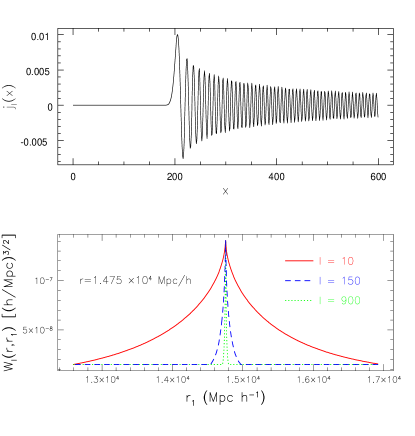
Figure 2: The top panel shows the spherical Bessel function of order $150$. The bottom panel shows the filters $W_{\ell}(r,r_{1})$ as functions of $r_{1}$, at fixed $r$, and three different values of $\ell$. We choose the spectral index $n=1$. Note that the filters become more and more peaked around $r_{1}=r$ as $\ell$ increases. The Bessel functions oscillate very fast and have to be sampled in many more points than $W_{\ell}$ to have an accurate numerical integration. For this reason the use of $W_{\ell}$ instead of $j_{\ell}$ drastically reduces the needed CPU time, as explained in the text.

Komatsu et al. (2003) (see also Komatsu, Spergel & Wandelt 2003) used this method to generate $300$ non-Gaussian maps at the WMAP resolution; their algorithm required about $3$ hours on $1$ processor of SGI Origin $300$ and $7.5$ GB of physical memory to generate a single map.

We developed an alternative algorithm which starts from the generation of the linear potential multipoles $\Phi^{\rm L}_{\ell m}(r)$, while we use the same technique as Komatsu et al. (2003) to account for the radiative transfer. We believe that the main advantages of the method we are going to describe w.r.t. the one just outlined can be the following: i) much less memory requirements, ii) a decrease of CPU time, iii) the possibility to more accurately resolve the last-scattering surface.

As we are going to see, we will obtain the multipole coefficients $\Phi^{\rm L}_{\ell m}(r)$ directly, i.e. without passing through the generation of the potential on a cubic grid. So we won’t need to convert from Cartesian to spherical coordinates, in order to harmonic transform $\Phi^{\rm L}(\mathbf{r})$ and, even more important, we won’t need to store big arrays containing the values of $\Phi^{\rm L}(\mathbf{r})$, calculated on the grid points. As the $\Phi^{\rm L}_{\ell m}(r)$ are Gaussian variables, to generate them we only need to know their correlation function. We have (see the Appendix):

$$\left\langle\Phi^{\rm L}_{\ell_{1}m_{1}}(r_{1})\Phi^{{\rm L}\star}_{\ell_{2}m_{2}}(r_{2})\right\rangle=\frac{2}{\pi}\delta_{\ell_{1}}^{\ell_{2}}\delta_{m_{1}}^{m_{2}}\int\!dk\,k^{2}P_{\Phi}(k)j_{\ell_{1}}(kr_{1})j_{\ell_{2}}(kr_{2})\;,$$ (12)

where $P_{\Phi}(k)$ is the primordial (i.e. unprocesssed by the radiation transfer function) power-spectrum of the gravitational potential, and $\delta^{i}_{j}$ is Kronecker’s delta. Since the multipoles $\Phi^{\rm L}_{\ell m}$ are correlated in real space, they cannot be generated directly. One possibility is to generate $\Phi^{\rm L}_{\ell m}(k)$ first, as they are independent Gaussian variables (see the Appendix, for an explicit calculation),

$$\left\langle\Phi^{\rm L}_{\ell_{1}m_{1}}(k_{1})\Phi^{{\rm L}\star}_{\ell_{2}m_{2}}(k_{2})\right\rangle=8\pi^{3}\frac{P_{\Phi}(k_{1})}{k_{1}^{2}}\delta^{D}(k_{1}-k_{2})\delta_{\ell_{1}}^{\ell_{2}}\delta_{m_{1}}^{m_{2}}\;,$$ (13)

($\delta^{D}$ being the Dirac delta function) and then transform $\Phi_{\ell m}(k)$ into $\Phi_{\ell m}(r)$, by Eq. (8).

As in this last equation, $\ell$ and $m$ are fixed and only $k$ varies for each integration, it is clear that this method does not require large memory: in fact, we never need to store all the values of $\Phi_{\ell m}(k)$ and $\Phi_{\ell m}(r)$ at the same time in physical memory.
Unfortunately, the spherical Bessel transform which allows the passage from $\Phi_{\ell m}(k)$ to $\Phi_{\ell m}(r)$ requires a lot of CPU time, as the $j_{\ell}(kr)$ are rapidly oscillating functions which have to be sampled in many points to ensure accurate numerical integration. The time needed to simulate one sky-map with this method is around $20$ hours on a Compaq server DS20E ($500$ Mhz), for $l_{max}=500$, and scales roughly as $l^{2}$. However, it is clear from the previous argument that the code could be greatly speeded up by avoiding the numerical integration of Eq. (8). This result can be achieved as follows: start from independent complex Gaussian variables $n_{\ell m}(r)$, characterized by the correlation function

$$\left\langle n_{\ell_{1}m_{1}}(r_{1})n^{*}_{\ell_{2}m_{2}}(r_{2})\right\rangle=\frac{\delta^{D}(r_{1}-r_{2})}{r^{2}}\delta_{\ell_{1}}^{\ell_{2}}\delta_{m_{1}}^{m_{2}}\;;$$ (14)

as shown in the Appendix, it is now possible to recover our Gaussian variables $\Phi^{\rm L}_{\ell m}(r)$, with the right correlation properties, by convolution,

$$\Phi^{\rm L}_{\ell m}(r)=\int\!dr_{1}\,r_{1}^{2}\,n_{\ell m}(r_{1})W_{\ell}(r,r_{1})\;,$$ (15)

where the filter functions $W_{\ell}(r,r_{1})$ are defined as

$$W_{\ell}(r,r_{1})=\frac{2}{\pi}\int\!dk\,k^{2}\,\sqrt{P_{\Phi}(k)}\,j_{\ell}(kr)j_{\ell}(kr_{1})\;.$$ (16)

In this work we will only consider models with a scale-free primordial density power-spectrum of the form $P(k)=Ak^{n}$, and we take $n=1$, in agreement with observational data (e.g. Spergel et al. 2003). In this case, when $r$ is fixed, the functions $W_{\ell}(r,r_{1})$ are smooth and differ from zero only in a narrow region around $r=r_{1}$ (see Figure 2). So, in order to accurately sample $W_{\ell}$ for their integration in Eq. (15) we only need to compute them in a few points, which considerably reduces the CPU time needed for the generation of $\Phi^{\rm L}_{\ell m}(r)$. The CPU time needed for the generation of a single sky-map at the WMAP resolution now goes down to less than one hour. In other words, by the latter method we work directly in real space, starting from white-noise coefficients and convolving them with suitable filters to produce the right correlation properties of the $\Phi^{\rm L}_{\ell m}(r)$. This technique for the generation of correlated random variables is well known in the literature (e.g. Salmon 1996; see also Peebles 1983). It is particularly efficient in our case, because, as it appears from Figure 2 the $W_{\ell}(r,r_{1})$ get more and more peaked around $r=r_{1}$ as $\ell$ increases.

3 Results and Conclusions

Let us summarize the various steps which define our numerical algorithm.

• Simulate the white-noise Gaussian fields $n_{\ell m}(r)$ directly in real space.
  

• Convolve them with the (pre-computed) filter functions $W_{\ell}(r,r_{1})$, to obtain the linear potential multipoles $\Phi^{\rm L}_{\ell m}(r)$.
  

• Compute the linear potential $\Phi^{\rm L}({\bf r})=\sum_{\ell m}\Phi^{\rm L}_{\ell m}(r)Y_{\ell m}({\hat{r}})$ and square it to obtain (modulo $f_{\rm NL}$) the non-Gaussian contribution to the gravitational potential, directly in spherical coordinates.
  

• Harmonic transform $\Phi^{\rm NL}({\bf r})$ to get $\Phi^{\rm NL}_{\ell m}(r)$.
  

• Convolve $\Phi_{\ell m}(r)=\Phi^{\rm L}_{\ell m}(r)+f_{\rm NL}\Phi^{\rm NL}_{\ell m}(r)$ with the (pre-computed) real-space radiation transfer functions $\Delta_{\ell}(r)$.

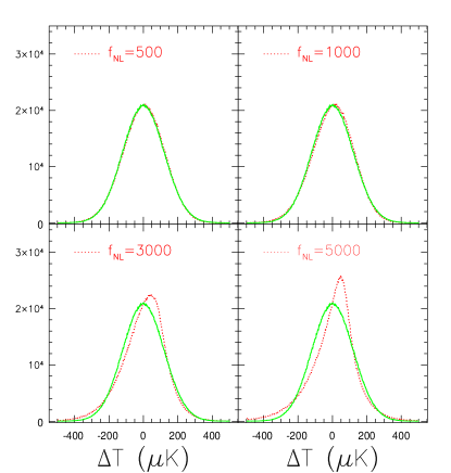
Figure 3: One-point PDF of temperature fluctuations obtained from a single simulated map with $l_{max}=3000$. Different panels show a comparison between the Gaussian realization ($f_{\rm NL}=0$) and the corresponding non-Gaussian one, for different values of $f_{\rm NL}$. Beam smearing has not been included here.

The form of $\Delta_{\ell}(r)$ suggests to generate the potential coefficients $\Phi^{L}_{\ell m}(r)$ for non-uniformly spaced values of the radial coordinate. In the final convolution, the real-space radiation transfer functions are in fact different from zero only near last scattering ($0.1\eta_{*}\lesssim\eta\lesssim 2\eta_{*}$, see Figure 1; $\eta_{*}$ is the conformal time, correspondingly $r_{*}=c\eta_{*}$), with a further contribution, coming from low redshifts and multipoles ($\ell\lesssim 50$, $r<5000\,h^{-1}$ Mpc, see the lower panel of Figure 1), due to the late-ISW effect. Therefore, we generated the multipoles $\Phi^{L}_{\ell m}(r)$ only for $\ell$ and $r$ belonging to the previously defined intervals. In this way we can increase the radial resolution in the selected regions and, at the same time, reduce the total number of points in our spherical grid (i.e. reduce the total number of evaluated $\Phi_{\ell m}(r)$), with a consistent reduction of the total CPU time needed. Moreover, since at low redshifts we need to consider only low multipoles, we may in this case reduce the pixel resolution when using HEALPix to perform the harmonic transforms, with further reduction of CPU time (this is because the value of the parameter $nside$ in HEALPix, which is directly related to the pixel resolution, has to be chosen in such a way as to verify the relation $l_{\rm max}<3\times nside$, and the calculation time for the harmonic transforms scales as $(nside)^{3}$).

In other words, our multipole approach enables to adapt the simulation grid to the optimal sampling of the physically relevant radial intervals (i.e. points where the radiative transfer is non-zero) and to reduce the CPU time needed for the generation of $\Phi^{L,NL}_{\ell m}(r)$. Moreover, we found it useful to split the high redshift contributions (SW effect, acoustic oscillations) from the low redshift contributions (late-ISW effect): in this way the simulation of the latter effects can be greatly speeded up, as they affect only the lower multipoles of the final map.

We have applied our algorithm to obtain some simulated temperature maps with different values of $\ell_{max}$, starting from a $\Lambda$CDM model with primordial spectral index $n=1$. The radial coordinate has been discretized with a step of $7.5\,h^{-1}$ Mpc in the regions where $\Delta_{\ell}(r)\neq 0$. In this way we generated $100$ potential multipoles in the radial interval $(r_{0}-2r_{*})\leq r\leq(r_{0}-0.1r_{*})$, for each $\ell$,$m$, $2\leq\ell\leq l_{\rm max}$, $0\leq m\leq\ell$, and we generated about $600$ potential multipoles with $r\leq 5000\,h^{-1}$ Mpc, for each $2\leq\ell\leq 100$, $0\leq m\leq\ell$.

To run our simulations we need $200$ Mb of physical memory when $\ell_{\rm max}=3000$; the final CPU time is reported in Table (1), where we also show the time needed for the harmonic analysis, at large $r$ only, as this is the most time-consuming part of our algorithm.

In Figure 3 we plot the PDF of temperature fluctuations, obtained from an original simulation with $\ell_{\rm max}=3000$, mainly for a comparison with the results contained in (Komatsu et al. 2003). In Figures 4,5 we show maps obtained from the same simulation, smoothed with different Gaussian beams at the resolution of COBE DMR, WMAP and Planck.

$\mathbf{\ell_{\rm max}}$	CPU time	Harmonic transform	nside
$300$	$8$ min	$6$ min	$128$
$500$	$40$ min	$32$ min	$256$
$750$	$1$ h $8$ min	$1$ h	$256$
$1500$	$8$ h $47$ min	$8$ h $20$ min	$512$
$3000$	$68$ h $45$ min	$67$ h $15$ min	$1024$

Table 1: CPU time needed to simulate a single map

The main purpose of obtaining simulated non-Gaussian CMB maps is that of providing a test-bed for the power of different statistical estimators, specifically designed to search for non-Gaussianity, in detecting the kind and the level of non-Gaussianity which is present in the maps. To this aim, all the possible extra effects, such as foreground contamination and instrumental noise of a specific experiment, which appear in the statistical analysis of real datasets should be properly taken into account. These aspects will be the analyzed in a forthcoming paper.

As already mentioned, there are various non-primordial cosmological effects which also imply a deviation from the Gaussian behaviour. These include systematic effects as well as some secondary sources of anisotropy. Among the future developments of the present algorithm is the possibility to include suitable kernels to account for some of these effects in the simulated CMB maps. This issue will be discussed elsewhere.

Figure 4: The left-hand side of this panel shows the same Gaussian realization, smoothed by three different beams. From top to bottom, the FWHM of the beams is $7^{\circ}$ (COBE), 13 arcmin (WMAP) and 5 arcmin (Planck). The right-hand side shows three corresponding non-Gaussian realizations, obtained from the Gaussian one by adding a non-linear coupling parameter $f_{\rm NL}=3000$ (such a high value of $f_{\rm NL}$ is chosen to make the non-Gaussian effects visible by eye). The model is a $\Lambda$CDM with primordial spectral index $n=1$. The primordial fluctuations have been COBE-normalized by CMBfast.

Figure 5: In this panel we show the same Gaussian maps of Fig. 4 on the left-hand side, while on the right-hand side we take $f_{NL}=-3000$. The remaining parameters are the same as in Fig. 4

Appendix A Derivation of useful formulae

A.1 Relation between $\Phi_{\ell m}(k)$ and $\Phi_{\ell m}(r)$

We start from the Fourier transform

$$\Phi(\mathbf{r})=\int\!\frac{d^{3}k}{(2\pi)^{3}}\,\Phi(\mathbf{k})\,e^{-i\mathbf{k\cdot r}}\;$$ (A1)

and we Rayleigh expand $\exp({-i\mathbf{k\cdot r})}$ in spherical harmonics,

$$\exp[-i\mathbf{k}\mathbf{\cdot r}]=4\pi\sum_{\ell}\sum_{m}(i)^{-\ell}Y_{\ell m}(\mathbf{\hat{k}})Y_{\ell m}^{*}(\mathbf{\hat{r}})j_{\ell}(kr)\;;$$ (A2)

we find:

$$\Phi(\mathbf{r}) = \frac{4\pi}{(2\pi)^{3}}\sum_{\ell}\sum_{m}(-i)^{\ell}Y_{\ell m}^{*}(\mathbf{\hat{r}})\int\!dk\,k^{2}\,j_{\ell}(kr)\times$$ (A3)

$$\;\;\;\;\;\;\;\;\;\;\;\times\int\!d\Omega_{\mathbf{\hat{k}}}\,Y_{\ell m}(\mathbf{\hat{k}})\,\Phi(\mathbf{k})\;.$$

Recalling that:

$$\Phi_{\ell m}(r)=\int\!d\Omega_{\hat{r}}\,\Phi(\mathbf{r})\,Y_{\ell m}^{*}(\hat{r})\;$$ (A4)

we can replace the previous expression for $\Phi(\mathbf{r})$ in the last formula [definition of $\Phi_{\ell m}(r)$] and expand also $\Phi(\mathbf{k})$ in spherical harmonics. We obtain

$$\Phi_{\ell m}(r) = \frac{1}{2\pi^{2}}\sum_{\ell_{1}\ell_{2}}\sum_{m_{1}m_{2}}(-i)^{\ell_{1}}\!\!\int\!d\Omega_{\mathbf{\hat{r}}}\,Y_{\ell m}^{*}(\mathbf{\hat{r}})\,Y_{\ell_{1}m_{1}}^{*}(\mathbf{\hat{r}})\times$$ (A5)

$$\!\!\!\!\!\!\!\!\!\!\!\!\!\!\!\times\int\!dk\,k^{2}\,j_{\ell_{1}}(kr)\,\Phi_{\ell_{2}m_{2}}(k)\int\!d\Omega_{\mathbf{\hat{k}}}\,Y_{\ell_{1}m_{1}}(\mathbf{\hat{k}})\,Y_{\ell_{2}m_{2}}(\mathbf{\hat{k}})\;.$$

It is now easy to see, by the orthonormality of spherical harmonics, that this reduces to Eq. (8).

A.2 Correlation function of $\Phi^{\rm L}_{\ell m}(k)$

Using the definition of $\Phi^{\rm L}_{\ell m}(k)$, we can write

$$\left\langle\Phi^{\rm L}_{\ell_{1}m_{1}}(k_{1})\Phi^{{\rm L}\star}_{\ell_{2}m_{2}}(k_{2})\right\rangle = \int\!d\Omega_{\mathbf{\hat{k}_{1}}}d\Omega_{\mathbf{\hat{k}_{2}}}\,\left\langle\Phi^{\rm L}(\mathbf{k_{1}})\Phi^{{\rm L}\star}(\mathbf{k_{2}})\right\rangle\,\times$$ (A6)

$$\;\;\;\;\;\times\;Y_{\ell_{1}m_{1}}^{\star}(\mathbf{\hat{k}_{1}})\;Y_{\ell_{2}m_{2}}(\mathbf{\hat{k_{2}}})\;.$$

From this we obtain:

$$\left\langle\Phi^{\rm L}_{\ell_{1}m_{1}}(k_{1})\Phi^{{\rm L}\star}_{\ell_{2}m_{2}}(k_{2})\right\rangle = (2\pi)^{3}P_{\Phi}(k_{1})\,\int\!d\Omega_{\mathbf{\hat{k}_{1}}}d\Omega_{\mathbf{\hat{k}_{2}}}\,\delta^{D}(\mathbf{k_{1}-k_{2}})\times$$ (A7)

$$\;\;\;\;\;\;\;\;\;\;\;\times\;Y_{\ell_{1}m_{1}}^{*}(\mathbf{\hat{k_{1}}})Y_{\ell_{2}m_{2}}(\mathbf{\hat{k}_{2}})\;.$$

Where we have used:

$$\left\langle\Phi^{\rm L}(\mathbf{k_{1}})\Phi^{{\rm L}\star}_{L}(\mathbf{k_{2}})\right\rangle=(2\pi)^{3}P_{\Phi}(k_{1})\delta^{D}(\mathbf{k_{1}-k_{2}})\;.$$ (A8)

Recalling now the integral representation of Dirac’s delta function,

$$\delta^{D}(\mathbf{k_{1}-k_{2}})=\frac{1}{(2\pi)^{3}}\int\!d^{3}\mathbf{r}\,\exp[i(\mathbf{k_{1}-k_{2}})\,\mathbf{\cdot r}]\;$$ (A9)

we can Rayleigh expand to obtain:
$\left\langle\Phi^{\rm L}_{\ell_{1}m_{1}}(k_{1})\Phi^{{\rm L}\star}_{\ell_{2}m_{2}}(k_{2})\right\rangle=$

$$=16\pi^{2}P_{\Phi}(k_{1})\sum_{\ell_{1}\ell_{2}\ell_{3}\ell_{4}}\sum_{m_{1}m_{2}m_{3}m_{4}}i^{\ell_{3}-\ell_{4}}\int drr^{2}j_{\ell_{3}}(k_{1}r)j_{\ell_{4}}(k_{2}r)\times$$

$$\;\;\;\;\;\;\;\;\times\int\!d\Omega_{\mathbf{\hat{r}}}\,Y_{\ell_{3}m_{3}}(\mathbf{\hat{r}})\,Y_{\ell_{4}m_{4}}^{*}(\mathbf{\hat{r}})\,\int\!d\Omega_{\mathbf{\hat{k}_{1}}}\,Y_{\ell_{1}m_{1}}^{*}(\mathbf{\hat{k}_{1}})\,Y_{\ell_{3}m_{3}}^{*}(\mathbf{\hat{k}_{1}})\times$$

$$\;\;\;\;\;\;\;\;\times\int\!d\Omega_{\mathbf{\hat{k}_{2}}}\,Y_{\ell_{2}m_{2}}(\mathbf{\hat{k}_{2}})\,Y_{\ell_{4}m_{4}}(\mathbf{\hat{k}_{2}})\;.$$ (A10)

By the orthonormality of spherical harmonics this reduces to

$$\left\langle\Phi^{\rm L}_{\ell_{1}m_{1}}(k_{1})\Phi^{{\rm L}\star}_{\ell_{2}m_{2}}(k_{2})\right\rangle = 16\pi^{2}P_{\Phi}(k_{1})\delta_{\ell_{1}\ell_{2}}\delta_{m_{1}m_{2}}\times$$ (A11)

$$\!\!\!\!\!\!\!\!\!\!\times\int\!dr\,r^{2}\,j_{\ell_{1}}(k_{1}r)\,j_{\ell_{2}}(k_{2}r)\;,$$

from which, recalling that

$$\int_{0}^{\infty}\!dr\,r^{2}\,j_{\ell}(k_{1}r)\,j_{\ell}(k_{2}r)=\frac{\pi}{2}\frac{1}{k_{1}^{2}}\delta^{D}(k_{1}-k_{2})\;,$$ (A12)

we finally obtain

$$\left\langle\Phi^{L}_{\ell_{1}m_{1}}(k_{1})\Phi^{L*}_{\ell_{2}m_{2}}(k_{2})\right\rangle=8\pi^{3}\frac{P_{\Phi}(k_{1})}{k_{1}^{2}}\delta^{D}(k_{1}-k_{2})\delta_{\ell_{1}}^{\ell_{2}}\delta_{m_{1}}^{m_{2}}\;.$$ (A13)

A.3 Correlation function of $\Phi^{L}_{\ell m}(r)$

According to the Wiener-Khintchine theorem,

$$\xi_{\Phi}(r)=\int\!\frac{d^{3}k}{(2\pi)^{3}}\,P_{\Phi}(k)\,e^{i\mathbf{k}\cdot(\mathbf{r_{1}-r_{2}})}\;,$$ (A14)

where $r=|\mathbf{r_{1}-r_{2}}|$, $\xi_{\Phi}(r)$ and $P_{\Phi}(k)$ are the correlation function and the power spectrum of primordial potential fluctuations, respectively. Expanding once again the exponential in spherical harmonics, we obtain

$$\xi_{\Phi}(r)=\frac{2}{\pi}\sum_{\ell=0}^{\infty}\sum_{m=-\ell}^{\ell}Y_{\ell m}(\hat{r}_{1})\,Y_{\ell m}^{*}(\hat{r}_{2})\,\int\!dk\,k^{2}\,P_{\Phi}(k)\,j_{\ell}(kr_{1})j_{\ell}(kr_{2})\;.$$ (A15)

By the definition of $\Phi_{\ell m}(r)$, we can write

$$\left\langle\Phi^{L*}_{\ell_{1}m_{1}}(r_{1})\Phi^{L}_{\ell_{2}m_{2}}(r_{2})\right\rangle=\int\!d\Omega_{\hat{r}_{1}}d\Omega_{\hat{r}_{2}}Y^{*}_{\ell_{1}m_{1}}(\hat{r}_{1})\,Y_{\ell_{2}m_{2}}(\hat{r}_{2})\,\xi_{\Phi}(r)\;.$$ (A16)

The final result is obtained by substituting $\xi_{\Phi}(r)$ by its expression (A15) and using the orthonormality of spherical harmonics,

$$\left\langle\Phi^{L*}_{\ell_{1}m_{1}}(r_{1})\Phi^{L}_{\ell_{2}m_{2}}(r_{2})\right\rangle=\frac{2}{\pi}\,\delta_{\ell_{1}}^{\ell_{2}}\,\delta_{m_{1}}^{m_{2}}\int\!dk\,k^{2}\,P_{\Phi}(k)j_{\ell_{1}}(kr_{1})j_{\ell_{2}}(kr_{2})\;.$$ (A17)

A.4 Derivation of $W_{\ell}(r,r_{1})$

Consider a Gaussian random field $\Phi^{\rm L}(\mathbf{r})$ with correlation function $\xi_{\Phi}(r)$. If $P_{\Phi}(k)$ is the corresponding power spectrum, then $\Phi(\mathbf{r})$ can be obtained as:

$$\Phi^{\rm L}(\mathbf{r})=\int\!d^{3}r_{1}n(\mathbf{r_{1}})\int\!\frac{d^{3}k}{(2\pi)^{3}}\sqrt{P_{\Phi}(k)}e^{i\mathbf{k}\cdot(\mathbf{r-r_{1}})}\;,$$ (A18)

where we have introduced the white-noise field $n(\mathbf{r_{1}})$:

$$\left\langle n(\mathbf{r_{1}})n(\mathbf{r_{2}})\right\rangle=\delta^{D}(\mathbf{r_{1}-r_{2}})\;.$$ (A19)

To find a similar expression for $\Phi^{\rm L}_{\ell m}(r)$ we define the quantities

$$W(\mathbf{r-r_{1}})\equiv\int\!\frac{d^{3}k}{(2\pi)^{3}}\sqrt{P_{\Phi}(k)}e^{i\mathbf{k}\cdot(\mathbf{r-r_{1}})}\;;$$ (A20)

now, as usual, we expand both $\Phi(\mathbf{r_{1}})$ and $W(\mathbf{r-r_{1}})$ in spherical harmonics and account for the orthonormality relations, to finally obtain

$$\Phi^{\rm L}_{\ell m}(r) = \int\!dr_{1}\,r_{1}^{2}\,n_{\ell m}(r_{1})W_{\ell}(r,r_{1})$$ (A21)

$$W_{\ell}(r,r_{1}) = \frac{2}{\pi}\int\!dk\,k^{2}\,\sqrt{P_{\Phi}(k)}\,j_{\ell}(kr)j_{\ell}(kr_{1})\;$$ (A22)

and

$$\left\langle n_{\ell_{1}m_{1}}(r_{1})n^{\star}_{\ell_{2}m_{2}}(r_{2})\right\rangle=\frac{\delta^{D}(r_{1}-r_{2})}{r^{2}}\delta_{\ell_{1}}^{\ell_{2}}\delta_{m_{1}}^{m_{2}}\;.$$ (A23)

References

- (1) Acquaviva, V., Bartolo, N., Matarrese, S., & Riotto, A. 2002, preprint astro-ph/0209156
- bard (80) Bardeen, J.M. 1980, Phys. Rev. D22, 1882
- (3) Bartolo, N., Matarrese, S., & Riotto, N., 2002, Phys. Rev. D65, 103505
- (4) Bernardeau, F., & Uzan, J.-P. 2002, Phys. Rev. D66, 103506
- (5) Bucher, M., & Zhu, Y. 1997, Phys. Rev. D55, 7415
- (6) Cayón, L., Martínez-González, E., Argüeso, F., Banday, A.J., & Górski, K.M. 2003, MNRAS, 339, 1189
- cb (87) Coles, P., & Barrow, J.D. 1987, MNRAS, 228, 407
- (8) Contaldi, C.R. & Magueijo, J. 2001, Phys. Rev. D63, 103512
- (9) Creminelli, P. 2003, preprint astro-ph/0306122
- (10) Dvali, G., Gruzinov, A., & Zaldarriaga, M. 2003, preprint astro-ph/0303591
- (11) Falk, T., Rangarajan, R., & Srednicki, M. 1993, ApJ, 403, L1
- (12) Gangui, A., Lucchin, F., Matarrese, S., & Mollerach, S. 1994, ApJ430, 447
- (13) Gangui, A, & Martin, J. 2000, Phys. Rev. D62, 103004
- (14) Górski, K.M., Hivon E., & Wandelt, B.D., 1999, in Proc. MPA/ESO Cosmology Conference “Evolution of Large-Scale Structure”, ed. by A.J. Banday, R.K. Sheth, L.N. da Costa. Garching, Germany: ESO, p. 37 [astro-ph/9812350]
- (15) Gupta, S., Berera, A., Heavens, A.F., & Matarrese, S. 2002, Phys. Rev. D66, 043510
- (16) Hansen, F.K., Marinucci, D., & Vittorio, N. 2003, preprint astro-ph/0302202
- (17) Hansen, F.K., Marinucci, D., Natoli, P., & Vittorio, N. 2002, Phys. Rev. D66, 063006
- kof (03) Kofman, L. 2003, preprint astro-ph/0303614
- (19) Komatsu, E., et al. 2003, submitted to ApJ[astro-ph/0302223]
- (20) Komatsu, E., & Spergel, D.N., 2001, Phys. Rev. D63, 063002
- komat (2) Komatsu, E., Spergel, D.N., & Wandelt, B.D. 2003, preprint astro-ph/0305189
- koma (02) Komatsu, E., Wandelt, B.D., Spergel, D.N., Banday, A.J., & Górski, K.M. 2002, ApJ566, 19
- (23) Linde, A.D., & Mukhanov, V. 1997, Phys. Rev. D56, R535
- (24) Lyth, D., Ungarelli, C., & Wands, D. 2003, Phys. Rev. D67, 023503
- (25) Lyth, D., & Wands, D. 2002, Phys. Lett., B524,5
- (26) Maldacena, J. 2002, preprint astro-ph/0210603
- (27) Martínez-González, E., Gallegos, J.E., Argüeso, F., Cayón, L., & Sanz, J.L. 2002, MNRAS, 336, 22
- (28) Matarrese, S., Verde, L., & Jimenez, R., 2000, ApJ, 541, 10
- mol (90) Mollerach, S. 1990, Phys. Rev. D42, 313
- (30) Moscardini, L., Matarrese, S., Lucchin, F., & Messina, A. 1991, MNRAS, 248, 424
- (31) Peebles, P.J.E., 1983, ApJ, 274, 1
- (32) Peebles, P.J.E., 1997, ApJ, 483, L1
- (33) Salmon, J. 1996, ApJ, 460, 59
- sal (90) Salopek, D.S., & Bond, J.R. 1990, Phys. Rev. D42, 3936
- sal (91) Salopek, D.S., & Bond, J.R. 1991, Phys. Rev. D43, 1005
- (36) Salopek, D.S., Bond, J.R., & Bardeen, J.R. 1989, Phys. Rev. D40, 1753
- (37) Santos, M.G. et al. 2003, MNRAS, 341, 623
- (38) Scaramella, R., & Vittorio, N. 1991, ApJ, 375, 439
- (39) Seljak, U., & Zaldarriaga, M. 1996, ApJ, 469, 437
- (40) Spergel, D.N., et al. 2003, submitted to ApJ[astro-ph/0302209]
- (41) Srednicki, M. 1993, ApJ, 416, L1
- (42) Verde, L., Wang, L., Heavens, A.F., & Kamionkowski, M. 2000, MNRAS, 313, 141
- (43) Verde, L., Jimenez, R., Kamionkowski, M., & Matarrese, S., 2001, MNRAS, 325, 412
- (44) Vio, R., Andreani, P., Tenorio, L., & Wamsteker, W. 2002, PASP, 114, 1281
- (45) Wang, L., & Kamionkowski, M. 2000, Phys.Rev. D61, 063504
- (46) Zaldarriaga, M. 2003, preprint astro-ph/0306006