A pulsar-atmosphere model for PSR 0656+14

Abstract

We present a pulsar-atmosphere (PA) model for modulated thermal X-ray emission from cooling magnetized neutron stars. The model synthesizes the spectral properties of detailed stellar atmosphere calculations with the non-uniform surface properties anticipated for isolated, aging radio pulsars, and general relativistic effects on photon trajectories. We analyze the archival Chandra observations of the middle-aged radio pulsar PSR 0656+14 with the PA model and find it is an excellent representation of the phase-averaged X-ray spectrum for a broad range of polar effective temperature $T_{p}$ and column density $N_{H}\simeq 10^{20}\ \mathrm{cm^{-2}}$. The spectral fits favor a sub-solar neutron star mass $M\lesssim 1.0\ M_{\sun}$, a large radius $R=15-16\ \mathrm{km}$ for a source distance $d\simeq 190\ \mathrm{pc}$, while retaining consistency with theoretical neutron star equations-of-state. The modulated spectrum constrains the angular displacement of the pulsar spin axis to $30\pm 2\arcdeg$ with respect to the line of sight.

1 Introduction

The discovery of modulated thermal X-rays in ROSAT observations of a handful of neutron stars (NSs) provided early evidence that the surface properties of these sources are inhomogeneous. Most NSs are rotation powered, and emit predominantly non-thermal X-rays generated exterior to the star in the pulsar magnetosphere (Becker & Trümper 1997; Possenti et al. 2002). Thermal X-rays from a few exceptional sources originate at the stellar surface and can be distinguished from magnetospheric contributions owing to their intermediate age: these are sufficiently aged to have experienced a decline in synchrotron activity, yet not so old that they are altogether too faint to be seen. The “Three Musketeers,” PSR 0656+14, PSR 1055-52 and PSR 0630+18 (Geminga) are relatively bright and weakly absorbed middle-aged radio pulsars which are among the earliest known thermal emitters (see Ögelman 1995 for a summary of ROSAT data). These sources remain excellent candidates for evaluating NS cooling models and surface characteristics, and are objects of continued interest in Chandra and XMM-Newton observations. Becker & Trümper (1997) tabulated the short catalog of confirmed thermal NSs from the combined ROSAT and ASCA data sets, which include the relatively young Vela pulsar. These X-ray spectra are found to be poorly described by a single blackbody and require in addition either a power-law or second blackbody component. The secondary “hard” thermal component is invoked to bridge the energy range between the “soft” thermal and power-law contributions and broadens the spectral distribution of the soft X-rays. This spectral model may be interpreted as thermal radiation from the entire stellar surface (soft) seen in relief against small hot-spots or otherwise externally heated polar regions (hard), plus the contribution from the magnetosphere at sufficiently high energies. In this picture, a careful measurement of the soft thermal component may allow for direct measurement of intrinsic stellar properties – radius $R$, characteristic temperature $T$, magnetic field and surface composition. This is quite challenging in practice because a reasonable interpretation of the spectrum requires a self-consistent model of the pulsar’s synchrotron continuum, stellar viewing angles and distance, in addition to the NS surface properties and the associated thermal radiation.

The principal difficulty posed by the soft X-ray spectra of these pulsars is in reconciling their modulated thermal emission and estimated distance with a model for the surface radiation. Owing in part to modest instrumental sensitivity to the peak energies of their relatively cool surface radiation $(0.1-1.0\ \mathrm{keV})$, measures of temperature, the intervening absorbing column and overall normalization (i.e., radius and distance) are mutually affected. These uncertainties can be compounded by discrepancies as large as a factor of $\sim 4$ from different techniques for estimating the distance to some sources. The average spectrum alone is not sufficient to deduce the temperature at the stellar surface, where local anisotropies likely play a significant role in the fraction and profile of the pulsed radiation; the energy dependent pulse profiles and modulation index are functions of the apparent viewing geometry and radiation beaming patterns, but are also dependent on the assumptions of the model for the relevant pulsar mechanism. In the absence of perfect energy resolution of the detector, the strength of the modulation that the observer infers also depends on the amount of interstellar absorption (Page 1995; Perna et al. 2000).

Models with two distinct thermal components provide acceptable fits to the mean X-ray flux of these sources, while more complicated surface temperature distributions also fare well. Page (1995) considered a smoothly varying blackbody distribution on the stellar surface and noted that a non-uniform temperature distribution implies increasing pulsed fraction with energy. The integration of such a dipolar temperature blackbody distribution is well represented by that of a single temperature within the limits of the PSPC data sets. X-ray pulsations are suppressed by gravitational lensing of the stellar surface for a dipolar field regardless of the details of radiation beaming. More complicated field geometries can be invoked to explain observed X-ray pulsation from the radio pulsars, but require unacceptable tuning of surface parameters (Page & Sarmiento 1996). The blackbody temperature configurations generate a pulsed fraction which increases with energy, and seems incapable of explaining either the non-monotonic growth in pulsed flux seen for the middle-aged radio pulsars observed with ROSAT and Chandra, or the phase shift in pulse synchronization seen at $0.3-0.5\ \mathrm{keV}$ in ROSAT observations. These may be partially resolved by beaming of radiation owing to intrinsic anisotropies to explain both phase-resolved measures.

Radiation emergent from a stellar atmosphere is inherently anisotropic regardless of the local temperature and magnetic field and, when combined with a non-uniform temperature profile, is capable of generating considerable pulsar modulation. The earliest effort to describe X-ray pulsations from NSs with magnetized plasma atmospheres was due to Pavlov et al. (1994). These models characterized the pulsar emission with small polar caps having uniform normal magnetic field while the remainder of the stellar surface was assumed to be too cool to contribute to the total flux. Zavlin et al. (1995) refined this approach and, in particular, generalized their calculation to include an inhomogeneous surface temperature distribution and dipolar field geometry. A significant result of this effort was the discovery of a “crossover” energy at which the pulsed X-ray spectrum could experience a phase-shift; this transition depends critically upon the details of the ionization equilibrium of cool NS atmospheres, and on the assumed surface temperature profiles and magnetic field geometry. The dipole model was found to be generally consistent with the ROSAT observations of the middle-aged radio pulsars. Meyer et al. (1994) made a detailed fit to the ROSAT observations of Geminga using partially ionized magnetic hydrogen atmosphere models; these authors considered a simple model for Geminga in which the temperature and magnetic field of the star were assumed homogeneous, effectively a magnetic monopole. The harder spectrum of the plasma atmosphere was not alone able to fully describe the ROSAT PSPC data and required the secondary polar cap component, albeit with much smaller effective emitting area than that deduced from dual blackbody fits.

Perna et al. (2001) derived pulsed X-ray spectra $(0.1-1.0\ \mathrm{keV})$ of rotating NSs from the surface temperature profiles of Heyl & Hernquist (1998a) by integrating the spectrum of a toy hydrogen atmosphere model (Heyl & Hernquist 1998b) at each point on the stellar surface. As found in the blackbody analysis, two thermal components were required to reproduce the averaged ROSAT spectra of the radio pulsars; the phase resolved properties of these spectra (pulsed fraction and pulse phase-lag with energy) were also reproduced by assuming the cap had different beaming properties than the remainder of the surface. More specifically, Perna et al. (2001) found that the behavior of the pulsed fraction, as measured by ROSAT PSPC, could be reproduced with the combination of a “pencil beam” component generated over the entire surface of the star, and a hotter “fan” beamed component, produced at the polar caps.

1.1 PSR 0656+14

X-ray emission from PSR 0656+14 was first detected with EXOSAT (Córdova et al. 1989); the suggested X-ray pulsations were later confirmed when evidence of X-rays pulsed at the radio period $P\sim 385\ \mathrm{ms}$ was found in the ROSAT PSPC observations described by Finley et al. (1992); this spectrum was inferred to be consistent with a blackbody $\mathit{T_{bb}}\simeq 9\times 10^{5}\ \mathrm{K}$ having normalization consistent with $R=10\ \mathrm{km}$ assuming a source distance $d=500\ \mathrm{pc}$. An optical counterpart was found in ESO observations $(m_{V}\sim 25)$ as reported by Caraveo et al. (1994), and optical pulsations displaced from the radio phase by 0.2 were recovered from later observations (Shearer et al. 1997). At X-ray energies, the correlation between spectral hardness and rotation phase suggests the pulsation originates in a non-uniform surface temperature distribution. Anderson et al. (1993) compare these PSPC data to contemporary ROSAT HRI observations $(0.15-2.0\ \mathrm{keV})$ and conclude from the modulated X-rays that the pulsed emission is probably no harder than the unpulsed spectrum. Greiveldinger et al. (1996) considered joint fits to the ROSAT and ASCA data sets found that the spectrum was best fit by two thermal components $T_{s}\simeq 8\times 10^{5}\ \mathrm{K},T_{h}\simeq 1.5\times 10^{6}\ \mathrm{K}$ for $N_{H,20}=1.7$ (expressed in units of $10^{20}\ \mathrm{cm^{-2}}$); the fit was significantly improved by inclusion of a power-law to accommodate the hard X-ray tail seen with ASCA. Edelstein et al. (2000) find that simultaneous fits to EUVE and ROSAT observations require both cooler temperatures for the soft thermal component $\mathit{T_{bb}}\simeq 3.6\times 10^{5}\ \mathrm{K}$ and larger absorbing columns $N_{H,20}=2.21$; continuing the fit to the thermal optical measurements (Pavlov et al. 1996, 1997) allow for larger $\mathit{T_{bb}}=(4.7-7.4)\times 10^{5}\ \mathrm{K}$ and smaller $N_{H,20}=(1.1-1.8)$, consistent with Greiveldinger et al. (1996). In either case, the hard thermal component is $\mathit{T_{bb}}\simeq(1.1-1.2)\times 10^{6}\ \mathrm{K}$. Chandra LETG observations (Marshall & Schulz 2002) find double blackbody fit parameters consistent with those of Greiveldinger et al. (1996). Optical photometry performed by Kurt et al. (1998) suggests the non-thermal optical flux has a spectral index roughly consistent with that of the hard X-ray emission; subsequent IR, optical and near UV measurements are consistent with a harder spectrum and evolution of the spectral index (Koptsevich et al. 2001). Pavlov et al. (2002) also made an ACIS-S observation in CC mode, and examined the joint fit with the earlier grating data $(0.2-6.0)\ \mathrm{keV}$. The resultant three component (BB+BB+PL) model is likewise consistent with that of Greiveldinger et al.; these authors find a fit to dual magnetic atmosphere models questionable because of the large derived stellar radius, assuming the source distance $d\simeq 500\ \mathrm{pc}$. HST observations of PSR 0656+14 provide strong evidence for identification of the optical counterpart (Mignani et al. 2000). The proper motion of this counterpart has been measured but, owing to the uncertainty in the pulsar velocity, does not constrain the source distance to better than a factor of $\sim 3$. The lower bound likewise agrees with the photometric estimate for this pulsar $(150-200\ \mathrm{pc})$ by Golden & Shearer (1999).

The energy dependence of the pulsed fraction of thermal X-rays has been measured from Chandra ACIS-S observations in the continuous clocking mode (Pavlov et al. 2002). The pulsed fraction does not grow continuously with energy, but rather exhibits lower pulsation from 0.5-1.0 keV when compared to either lower or higher energy intervals; this property is a significant constraint on comprehensive models for the X-ray emission. The earlier ROSAT observations show an increase in the pulsed fraction with energy, and is seemingly inconsistent with any decrease in pulsation on this same interval. Both datasets reveal an apparent phase shift in the pulsed thermal X-rays although the magnitude of the phase displacement differs and energies affected differ between the two observations ($\sim 0.8$ keV in ROSAT, $\gtrsim 1.0$ keV in Chandra). Possenti et al. (1996) evaluated the pulsed fraction predicted by the dual temperature blackbody model and concluded from the PSPC data that the measured $\sim 9\%$ on $(0.1-2.4)\ \mathrm{keV}$ could be reconciled with the viewing geometry $\chi=30$ estimated by Rankin (1993), but only for gravitational redshift $z\lesssim 0.15$.

In this article, we describe the synthesis of light element fully ionized plasma atmosphere models of Lloyd (2003) with realistic NS temperature and field configurations derived from NS crustal conductivities (Heyl & Hernquist 1998a). The resulting model yields self-consistent pulse properties of the pulsar surface radiation and provides substantial improvement over previous efforts to describe pulsed thermal X-rays from NSs. We compare the pulsar atmosphere model to archival Chandra data for PSR 0656+14, and examine the extent to which our model provides an adequate solution to both the average spectral envelope of this pulsar and the energy-dependent pulsed fraction. The pulsar model is capable of reproducing the average X-ray spectrum without an explicit secondary thermal component, but fails to reconcile the observed pulsed fraction.

We organize our discussion as follows: the pulsar-atmosphere (PA) model is detailed in §2. The extraction and reduction of the Chandra LETG and ACIS-S observations is described in §3.1, followed by the results of our spectral analysis in §4.

2 Pulsar atmospheres

The surface distribution of effective temperature on a NS depends on the local magnetic field strength and its inclination with respect to the surface normal vector, and is prescribed by the conductive properties of the magnetized neutron star crust (e.g. Greenstein & Hartke 1983; Hernquist & Applegate 1984; Hernquist 1984; Heyl & Hernquist 1998a). Both the field and temperature distributions are parameterized by their values at the magnetic pole. For a body-centered dipolar magnetic field, the surface field strength at magnetic colatitude $\theta_{p}$ is

$$B(\theta_{p})=\frac{B_{p}}{2}\sqrt{1+3\cos^{2}{\theta_{p}}}\ .$$ (1)

The magnetic field vector at this point is inclined with respect to the local normal (i.e. radial vector) by an angle $\psi$

$$\cos{\psi}=\frac{2\cos{\theta_{p}}}{\sqrt{1+3\cos^{2}{\theta_{p}}}}\ .$$ (2)

Thermal conductivity in the magnetized NS crust varies with the magnetic field density and direction, resulting in a smooth variation of effective temperature from the magnetic pole to equator; for fields $B_{p}\gtrsim 10^{11}\ \mathrm{G}$, Heyl & Hernquist (1998a) find:

$$\mathit{T_{eff}}(\theta_{p})=T_{p}\left[\left(\frac{B}{B_{p}}\right)^{1/5}\frac{4\cos^{2}{\theta_{p}}}{1+3\cos^{2}{\theta_{p}}}\right]^{1/4}\ .$$ (3)

We may optionally superimpose the radiation from heated polar caps on the pulsar temperature distribution. The cap dimension is described by the angular radius $\theta_{c}$, and its intensity pattern is modeled with a normal, uniform surface magnetic field $B_{p}$ and constant effective temperature $T_{c}$ on the magnetic colatitude interval $[0,\theta_{c}]$. Radiation from the polar cap will supersede that of the pulsar distribution for $\theta_{p}$ in this range. We simplify integration of the total surface emission in the ordinary dipole field geometry by taking advantage of the axial symmetry of the $B$ and $T$ distributions. The radiation field at an arbitrary point on the stellar surface can be mapped into the equivalent point on a narrow strip of magnetic longitude extending from the (magnetic) pole to equator which we discretize into $\sim 20$ surface elements having uniquely defined local properties $\vec{B},\mathit{T_{eff}}$ from equations (1-3). Each element is modeled using the computational methods described in Lloyd (2003) to derive the asymmetric thermal intensity patterns for a hydrogen plasma atmosphere with these parameters. The model intensities $I_{E}(\vec{k})$ from all elements are tabulated for interpolation of the radiation profile from an arbitrary point on the NS surface. The radiation field is fully symmetric about the magnetic equator, including the two antipodal caps.

2.1 Phase resolved model spectra

The viewing geometry of the NS is defined by two angles: the angle $\chi$ between the line of sight (LOS) and the pulsar spin axis $\vec{P}$, and the relative angular displacement $\xi$ of the magnetic dipole axis $\vec{B}_{dip}$ from $\vec{P}$. Consequently, the angle $\alpha$ between the magnetic dipole axis and the LOS varies with phase angle $\gamma\equiv 2\pi t/P$:

$$\vec{B}_{dip}=(\sin{\chi}\cos{\xi}-\cos{\chi}\sin{\xi}\cos{\gamma},-\sin{\xi}\sin{\gamma},\cos{\alpha})$$ (4)

where

$$\cos{\alpha}=\cos{\chi}\cos{\xi}+\sin{\chi}\sin{\xi}\cos{\gamma}.$$ (5)

Any particular viewing geometry for which $\chi$ or $\xi=0$ is degenerate, and fails to produce modulation of the surface emission in the dipole model. Results for choices of $\chi$ or $\xi$ which exceed $\pi/2$ are equivalent to those for which the angle is subtracted from $\pi$.

Calculation of the phase-resolved flux proceeds from integration of the intensity vectors coincident with a distant observer’s LOS from a large number of points on the stellar surface. Two coordinate systems are required, and computation of the model spectrum is facilitated by the translation from viewing or integration coordinates defined by a fixed LOS to NS surface coordinates defined with respect to the dipole axis. This derivation proceeds in Cartesian coordinates and assumes $\hat{l}=(0,0,-1)$ for the LOS. To deduce the correct intensity contribution from an arbitrary point on the star, we require three surface coordinates: the local magnetic colatitude $\theta_{p}$, and the direction of the intensity vector which is parallel to the LOS at distance and given by the pair of angles $(\theta_{b},\phi_{b})$ in the NS frame. The global geometry is illustrated in Figure 1. The remainder of our derivation describes recovery of this angular information from the dipole pulsar model for arbitrary $\chi,\ \xi$ and $\gamma$.

Figure 1: The global viewing geometry is specified by the pair of angles $\chi,\xi$. The dipole axis sweeps the dashed curve as the star rotates though phase angle $\gamma$. $\vec{P}$ is fixed and coplanar with the line of sight $(-\hat{z})$ while $\vec{B_{dip}}$ is coplanar with the LOS and spin axis $\vec{P}$ when $\gamma=0$ or $\pi$. Any surface element having normal $\hat{n}$ is referenced in two coordinate systems: $(\alpha,\theta_{p})$ for some phase in the pulsar coordinates, and by $(\theta,\phi)$ in the surface integration coordinates. $\phi$ is measured with respect to the projection of $\hat{n}$ onto the $\hat{x}-\hat{y}$ plane (shown here as $\hat{n}_{xy}$).

The precise intensity contribution from each surface element varies with rotational phase for a given viewing geometry, but the overall configuration of surface elements remains fixed. In a given phase, each surface element is identified by a pair of polar integration coordinates $(\delta,\phi)$ where $\delta$ is the angle between the intensity vector from the surface which intersects the detector $[0,\pi/2]$ and the local normal vector, and the circumpolar angle $\phi$ is on the interval $[0,2\pi]$. The LOS is the pole of this coordinate system. The extent of the visible surface is defined by $\delta=\pi/2$. Note that, for relativistic stars, photons with trajectories $\delta=\pi/2$ in these coordinates emerge from surface latitudes $\theta>\pi/2$; in such cases the star is self-lensing and has larger exposed radiative area than geometric area for a hemisphere; for a non-relativistic star $\theta\rightarrow\delta$. To provide an absolute reference for $\phi$, the prime meridian is defined such that the spin axis $\vec{P}$ and LOS are coplanar with all normal vectors having $\phi=0$ regardless of phase angle; for $\gamma=0$, the magnetic dipole vector is likewise coplanar with the spin and LOS.

Figure 2 summarizes the geometry at a given surface element. In our integration coordinates, the local normal vector at the point $(\theta,\phi)$ on the stellar surface is

$$\hat{n}=(\sin{\theta}\cos{\phi},\sin{\theta}\sin{\phi},\cos{\theta})$$ (6)

and has magnetic colatitude given by

$$\cos{\theta_{p}}=\hat{B}_{dip}\cdot\hat{n}$$ (7)

The magnetic field at $\hat{n}$ is $\vec{B}=3\cos{\theta_{p}}\hat{n}-\vec{B}_{dip}$ (cf. eqn 2). In the atmosphere description of the individual surface elements, the local azimuthal reference is $\phi=0$ for coplanar $\hat{n},\hat{B}$. The angle between the LOS and $\hat{n}-\vec{B}$ plane is

$$\cos{\phi_{b}}=\hat{m}\cdot\hat{v}$$ (8)

where $\vec{v}=\hat{B}-\hat{n}\cos{\psi}$ and $\hat{m}=-(\cos{\theta}\cos{\phi},\cos{\theta}\sin{\phi},-\sin{\theta})$ are the projections of $\vec{B}$ and the LOS onto the local tangent plane. $\phi_{b}$ is the azimuthal angle the intensity vector forms with respect to the magnetic field axis and local normal vectors (Lloyd 2003). Note that the intensity vector and local normal are coplanar with the LOS. To complete our definition of the intensity vector, we measure the angle $\theta_{b}$ between the desired intensity vector at the NS surface and the local normal, given by the general relativistic “ray-tracing” integral (Page 1995):

$$\theta_{b}(x)=\int_{0}^{1/2}x\left[\frac{1}{4}\left(1-\frac{1}{R_{*}}\right)-\left(1-\frac{2v}{R_{*}}\right)v^{2}x^{2}\right]^{-1/2}{\>\rm d}v$$ (9)

where $x\equiv\sin\delta$, $R_{*}\equiv R/R_{S}$ and the Schwarzschild radius $R_{S}\equiv 2GM/c^{2}$.

Figure 2: The surface element defined at the point referenced by $\theta,\phi$ in the integration coordinates. The intensity $\vec{I}$ intersects the detector at infinity and the angles $\delta$ and $\theta$ are mutually defined by eqn. (9). Individual surface elements are computed using the local $\vec{B}$ and $\mathit{T_{eff}}$ defined by the global (dipolar) magnetic field geometry. The angular intensity patterns are generally anisotropic, and the local azimuthal angle $\phi_{b}$ is required for interpolation over the emission from the table of computed elements.

The intensity $I_{E}(\theta_{b},\phi_{b})$ from any integration element is step-wise interpolated from the table of surface elements. The analytic surface temperature distribution (3) poorly approximates the local flux for $\theta_{p}\gtrsim 85\arcdeg$; this region contributes $\ll 1\%$ of the total surface emission and integration elements within this interval will be considered “dark” making no contribution to the total. The phase resolved spectrum is

$$F_{E}(\gamma)=\pi\left(\frac{R}{d}\right)^{2}\int_{0}^{2\pi}\frac{{\>\rm d}\phi}{2\pi}\int_{0}^{1}{\>\rm d}(x^{2})\ I_{E}(\theta(x),\phi)$$ (10)

The prefactors in eqn (10) normalize the total flux to a distant source, where $R$ and $d$ are respectively the stellar radius and source distance. Relativistic self-lensing effects are included in the intensity integration described above, while the gravitational redshift will be accounted for when fitting the model to the Chandra data (§4). The phase averaged spectrum is

$$F_{E}=\frac{1}{2\pi}\int_{0}^{2\pi}{\>\rm d}\gamma F_{E}(\gamma)$$ (11)

The average spectrum is typically calculated over $\sim 20-30$ phases of the pulsar rotation $\gamma=[0,\pi]$ while the integration of total flux is performed by interpolating over on the order of 10,000-20,000 surface elements per phase. The most useful representation of the phase-resolved spectrum is the energy dependent pulsed fraction (PF)

$$PF_{E}=\frac{F_{E}^{max}-F_{E}^{min}}{F_{E}^{max}+F_{E}^{min}}$$ (12)

In eqn (12) the “bright” $(F_{E}^{max})$ and “dim” $(F_{E}^{min})$ phases are $\gamma=0$ and $\pi/2$ respectively which are correct at X-ray energies for pulsar models in the absence of a finite polar cap. For cap models with finite temperature contrast, the assignment of $\gamma$ for bright and dim may be reversed for portions of the X-ray flux (Perna et al. 2001). This is equivalent to a phase change in the pulse synchronization for different spectral components and is distinguished in these models by a negative $PF$. For a realistic detector the pulsed fraction must be evaluated over a finite band:

$$PF_{E}(\Delta E)=\int_{E}^{E+\Delta E}PF_{E}{\>\rm d}E$$ (13)

Instrumental efficiency and absorption in the ISM are energy dependent and must therefore be included in the calculation of the integrated pulsed fraction (Page 1995; Perna et al. 2000). As with gravitational redshift of the spectrum, these effects will be incorporated into spectral model from within the XSPEC software package. The pulsed fraction predicted in the PA model and others increases with large $R$, owing to the diminished effect of self-lensing.

For a given polar magnetic field strength, the spectral model is parameterized by the polar temperature of the pulsar distribution $T_{p}$, the angular size $\theta_{c}$ and temperature $T_{c}$ of the heated cap region, and the viewing angles $\chi$ and $\xi$. The pulsar atmosphere spectra are written in the FITS table format for use in the XSPEC software package (Arnaud 1996). Polar caps may take angular radii up to $13\arcdeg$ for temperatures $\log{T_{c}}=5.7-6.5$, while the underlying pulsar pole temperature takes values $\log{T_{p}}=5.4-6.0$. The “bright” and “dim” phase spectra are also included in the table to facilitate integration of the pulsed fraction. The pulsar viewing angles $\chi,\xi$ may assume values from $0-90\arcdeg$.

3 Data reduction

3.1 Low energy transmission grating spectrum

PSR 0656+14 was observed with the Chandra HRC-LETG configuration (the combination of the High Resolution Camera imaging detector and the Low Energy Transmission Grating - Brinkman et al. 2000) on 1999 November 28, with a total exposure time of 38 ks (ObsID 130). We retrieved the primary data products of this observation (i.e. standard filtered events files, aspect solution, and bad-time/pixels filters) from the public Chandra Data Archive, and extracted a dispersed spectrum of the source with negative ande positive orders co-added, and the background spectrum, using the Ciao (Chandra Interactive Analysis of Observations) software (standard shape and size extraction regions were used for both source and background). Ancillary Response Functions (ARFs) for negative and positive orders were also built with Ciao, and then co-added, while for the redistribution matrix the HRC-LETG combination does not allow us to resolve orders, so our final co-added spectrum contains counts from all possible dispersed orders. However, contamination from orders higher than the first, is only relevant at wavelengths longer than $\sim 80$ Å ($\sim 0.15$ keV), which we do not use in our analysis. For the purpose of spectral analysis, we then built (with Ciao) negative and positive 1st order HRC-LETG Ancillary Response Functions (ARFs), and then co-added them. For the Redistribution Matrix Function (RMF), instead, we used the “canned” 1st-order HRC-LETG RMF distributed with the Chandra CALibration Data Base (CALDB).

The total number of background subtracted counts in the source dispersed spectrum, between 0.15 and 1.5 keV (the energy range used in our spectral analysis) is 9230, corresponding to a signal to noise per resolution element of $\Delta\lambda=0.05$ Å, of SN = 2.5 (6 counts per resolution element). Such a low number of counts per resolution element does not allow us to search for narrow absorption or emission features in the spectrum or to apply the $\chi^{2}$ statistics to fit models for the continuum emission to the unbinned spectrum. We then grouped our spectrum allowing a minimum of 50 counts per new grouped channel, and performed spectral fitting by using the fitting package XSPEC on background subtracted data.

3.2 ACIS-S3 CCD spectrum

PSR B0656+14 was observed for 25 ks on 15 December 2001, using the ACIS detector in continuous-clocking (CC) mode (ObsID 2800). In this mode, one imaging dimension is sacrificed in order to provide fast read-out of the CCD. The resulting data consist of one row of events for which each pixel value represents the sum of events from the associated CCD column, with a time resolution of $\sim 3$ ms. The target was centered on the S3 chip, which is a backside-illuminated device. The energy resolution is $\Delta E/E\sim 0.1$ at 1 keV, and this varies gradually with row number.

Source and background spectra were extracted from the data using the dmextract routine in Ciao. Source events were extracted from a region extending $\sim 1.8$ arcsec on either side of the projected position of PSR B0656+14, while background events were taken from a $\sim 48$ arcsec region adjacent to the pulsar. Spectra were grouped to contain a minimum of 25 counts in each bin.

Calibration products for spectra obtained in CC-mode do not currently exist. As a result, we used spectral response and effective area files created for a Timed-Exposure (TE) mode observation of PSR B0656+14 carried out on the same day, with the same pointing and detector position configuration, as for the CC-mode observation. Spectra from the TE-mode data were not used in these analyses because the count rate for the pulsar is sufficiently high ($2.07\pm 0.01{\rm\ ct\ s}^{-1}$ in the CC-mode data) that pileup effects significantly distort the spectrum.

3.3 Timing analysis

For investigation of the pulsed X-ray emission from PSR B0656+14 we extracted event times from a 1 x 1.5 arcsec² box which included pixels for which the count rate was a factor of 10 or more higher than the average for pixels outside the region of the pulsar location. Event times were corrected from readout times to arrival times by correcting for time offset effects from dither of the spacecraft and any motions of the Science Instrument Module, following the science analysis thread on CC-mode time corrections with Ciao. These times were then corrected to the solar system barycenter with the axbary task, using the nominal coordinates of the pulsar (RA₂₀₀₀: 06:59:48.122, Dec₂₀₀₀: +14:14:21.53).

A search for periodicity around the expected frequency of 2.59805548 Hz, based on the ephemeris of Chang & Ho (1999), was carried out using the $Z_{n}$ test (Buccheri et al. 1983). The pulsations were easily detected with $f=2.598054\pm 1.5\times 10^{-6}$ Hz. Absolute phases for each event were then calculated based on the above ephemeris (see Table 1). Pulse profiles for selected energy ranges are shown in Figure 3, along with the measured pulsed fraction for each profile, defined here as $p=(M-m)/(M+m)$ where $M$ is the maximum number of counts in the folded lightcurve and $m$ is the minimum.

Figure 3: X-ray lightcurves for PSR 0656+14 accumulated with Chandra ACIS, integrated on representative energy intervals. The pulsed fraction for each band is indicated in the upper left corner of the panel. The pulse profiles are irregular and are not well described by the high degree of symmetry intrinsic to our pulsar atmosphere model. The energy intervals are the same as found in Pavlov et al. (2002).

Table 1: PSR B0656+14 Ephemeris

Quantity	Value
Epoch (MJD)	50701.000002341
$f$ (Hz)	2.5981054226747
$\dot{f}({\rm Hz\ s}^{-1})$	$-3.71150\times 10^{-13}$
$\ddot{f}({\rm Hz\ s}^{-2})$	$8.33\times 10^{-25}$

4 Spectral analysis

Radio measurements of PSR 0656+14 suggest the pulsar has a magnetic field strength $B\simeq 4.7\times 10^{12}\ \mathrm{G}$ in the dipole braking model. Its spectrum has been observed at optical and UV energies, and Ramanamurthy et al. (1996) reported the possible detection of $\gamma$-ray pulsations at the 385 ms rotation period in the EGRET data. Neither atomic (ionization) nor cyclotron features are evident at any wavelength, and a direct measure of the surface magnetic field is not possible. For this analysis we assume that the surface polar strength does not differ from that estimated from radio measurements, consistent with the absence of either electron or proton cyclotron absorption at X-ray energies. Our analysis proceeds from the combined LETG ($0.3-0.9\ \mathrm{keV}$) and ACIS-S ($0.4-6.0\ \mathrm{keV}$) data sets.

A uniform (single component) blackbody spectrum will not produce modulated flux, and both single temperature blackbody (BB) and uniformly magnetized neutron star atmosphere spectra (ATM) also fail to reproduce the phase-averaged Chandra spectrum; these elementary models can be discarded immediately. The next simplest alternative which does permit modulation is the composite of either uniform thermal emission and a power-law (PL) component or a double-blackbody (DBB) configuration with finite temperature contrast. The ACIS spectrum is non-thermal above 2.0 keV; the DBB model must also include the PL component to obtain a satisfactory fit. We fixed the power-law component to be consistent with the spectral fit to optical measurements as described by Kurt et al. (1998). The ATM+PL yields a formally acceptable fit to these data, although the resultant power-law amplitude is sufficiently small that temperature variation is required to account for the $PF$ below 2.0 keV, even for 100% pulse index in the PL flux at these energies. The extent to which the non-thermal emission is pulsed is arbitrary in this model; however, no evidence of pulsations above $2\ \mathrm{keV}$ was found in RXTE observations of this source (Chang & Ho 1999), and we assume the non-thermal flux is unpulsed at all energies in the Chandra data. It is possible that finite pulsation of non-thermal emission at energies $\lesssim 6.0\ \mathrm{keV}$ could remain consistent with the RXTE measurement. The combined BB+PL is a poor representation of these X-ray data, and we find that although the DBB plus PL model provides an acceptable fit to the average spectrum ($T_{1}=0.85\ \mathrm{MK}$, $T_{2}=1.5\ \mathrm{MK}$, $A_{2}/A_{1}=3.4\times 10^{-2}$ Pavlov et al. 2002), this configuration does not reproduce the observed pulsed fraction at 0.5-1.0 keV for any choice of viewing angles.

We evaluated the combined Chandra data sets with a grid of PA model spectra for a grid of mass $M=(0.4,1.0,1.4)M_{\sun}$, radius $R=10-16\ \mathrm{km}$ in steps of 1 km, and temperature $\log{T_{p}}=5.4-6.0$ in steps of 0.1 dex, and we obtained good spectral fits ($\chi^{2}/\mathit{dof}\lesssim 1.0$) with each pair of $M,R$ for a range of viewing angle $\chi$ on the interval $2-44\arcdeg$. Here, we have assumed $\chi=\xi$ to reduce the parameter space, which maximizes the pulsed fraction while demanding the magnetic pole sweep through the line of sight. For each pairing, we assumed the non-thermal emission was well represented by a power-law having index $\gamma=1.5$. The spectral fits favor low absorbing columns $N_{H,20}=1.0-1.2$. From this grid, we selected those models which generate the observed pulsed fraction from 0.3-0.5 keV, and maximized the source distance (Figure 4). The PA model provides a good fit to the observed average spectrum for a range of $T_{p}=0.48-0.62\ \mathrm{MK}$ $(T_{p}^{\infty}=0.45-0.5\ \mathrm{MK})$ yielding a source distance $100\lesssim d\lesssim 250\ \mathrm{pc}$. The thermal component $PF(0.3-0.5\ \mathrm{keV})\lesssim 0.32$ over the grid, but also $\lesssim 0.36$ above 1.0 keV. The deficit of pulsed emission predicted by the PA model may be accounted for by finite modulation of the non-thermal radiation at these energies at the level of $\sim 70\%$.

Figure 4: The grid of PA+PL models, organized by mass and radius. Each curve is the locus of predicted $PF$ and $d$ for each choice of $M,R$ and $\chi$. 16 km tracks for each mass are labeled, and curves for lower radii (in 1 km increments) are displaced to lower $d$ for large inclinations $\chi$. For each curve, the viewing angle $\chi(=\xi)$ increases from $\sim 2\arcdeg$ from the bottom of the figure to $\sim 35\arcdeg$ at the top. Well-defined spectral fits were obtained for $\gamma=1.5$ and $N_{H}=1.0-1.2\times 10^{20}\ \mathrm{cm^{-2}}$. Distance and $PF$ limits restrict further analysis to those models in the rectangular area. The best PA+PL models gives a 15-16 km stellar radius for $d\simeq 190\ \mathrm{pc}$, favors a sub-solar neutron star mass and implies $\chi\simeq 30\arcdeg$.

The distance and pulse index constraints favor sub-solar NS masses and large stellar radii. To proceed, we consider in detail the PA model results for a particular choice which satisfies our constraints, $M=0.4M_{\sun}$ and $R=16\ \mathrm{km}$. We recovered $PF(0.3-0.5\ \mathrm{keV})$ within the measured uncertainties in our models for $T_{p}\simeq 0.5\ \mathrm{MK}$ and $\chi=30\pm 2\arcdeg$. The unfolded spectral model is illustrated in Figure 5.

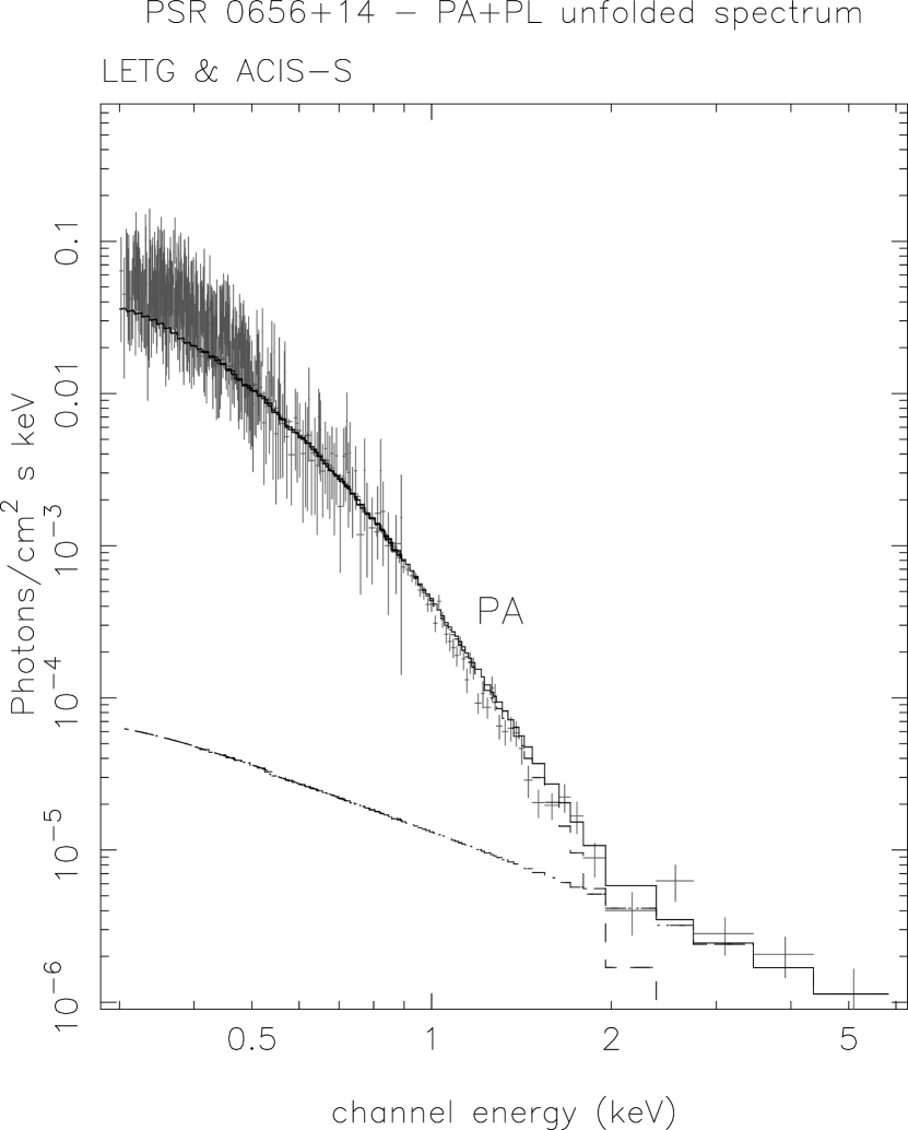
Figure 5: The unfolded model and spectrum for $R=16$ km enclosing 0.4 $M_{\sun}$ at $d\simeq 190\ \mathrm{pc}$. These stellar parameters are consistent with several equations-of-state (Lattimer & Prakash 2001). Non-thermal emission dominates above 2 keV and is arbitrarily pulsed in our model.

The PA model flux peaks at a lower energy compared to a uniform surface at $T_{p}$ and has a broader spectral envelope owing to the area-weighted average of the surface distribution, allowing for excellent representation of the X-ray spectrum. The PA component does not over-estimate the optical flux of the pulsar, which has a non-thermal spectrum (Figure 6).

Figure 6: The two component optical model for PSR 0656+14. Data points are those compiled in Koptsevich et al. (2001). The optical flux is dominated by the non-thermal component, described here by the same power-law used to model the hard X-rays in the Chandra data. The thermal component has an approximately Rayleigh-Jeans spectrum and does not over-produce optical flux. The broad feature centered at $\sim 7\times 10^{15}\ \mathrm{Hz}$ is proton cyclotron absorption in the hydrogen plasma.

For $\chi=\xi$, the ideal pulsed fraction predicted by the model exhibits two trends with $R$ and $\chi$. Spectral fits for fixed $R$ produce larger net pulsed fraction for increasing $\chi$ owing to larger flux contrast as the bright magnetic pole is inclined from the line of sight. This has the incidental effect of requiring slightly larger model normalization, favoring lower $d$ as the overall flux is reduced on average. Second, the magnitude of self-lensing is reduced by either increasing the radius or reducing the stellar mass, thereby increasing the pulsed fraction at all energies. The effective emitting area of the star grows with increasing $R^{\infty}=R(1+z)$, and spectral fits to the pulsar spectrum accommodate greater source distance.

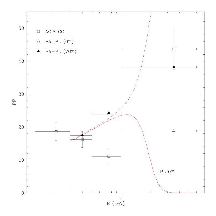
Figure 7: The pulsed fraction for PSR 0656+14. The measured net $PF$ integrated from 0.13-6.0 keV is 13.2%. The convolved model $PF$ for the parameters of Figure 5 (open triangles) fails to reproduce the pulsed fraction from 0.5-1.0 keV. The solid curve illustrates the thermal contribution to the pulsed fraction for the same model. Modulation of $\sim 70\%$ in the PL component is sufficient to reproduce the measured $PF$ above 1 keV (filled triangles), but does not lower the predicted pulsation from 0.5-1.0 keV; the dashed curve illustrates the $PF(E)$ for this model. Calibration issues prevent using the spectrum below 0.3 keV, although these data are expected to faithfully represent the pulsed fraction at lower energies.

The energy dependence of the pulsed fraction (Figure 7) is an especially restrictive constraint on models for thermal X-ray production for PSR 0656+14. Page (1995) demonstrated how continuous variation of the surface temperature naturally produces a $PF$ which increases monotonically with energy. We attempted to model the pulsed fraction at all energies by forcing finite polar cap emission with temperature contrast $T_{c}>T_{p}$. While formally acceptable fits to the phase-averaged spectrum can be obtained from these model combinations, the result in each case demands that the “soft” thermal component have both very low $T_{p}$ and large stellar radius. For example, we recovered $\theta_{c}\simeq 2\arcdeg$ for $T_{p}=0.4\ \mathrm{MK}$ and $T_{c}=1.0\ \mathrm{MK}$ held constant during the fit; by evaluating the $PF$ over a grid of $(\chi$, $\xi)$ we found the most compatible values were $\chi=80\arcdeg$, $\xi=50\arcdeg$. The PA & cap model is nevertheless unacceptable as a comprehensive representation for the pulsar thermal radiation: the radius expected for the relatively cool $T_{p}$ component is 65 km for $d=200\ \mathrm{pc}$; alternatively, the pulsar must have a distance of only 30 pc for the canonical radius $R=10\ \mathrm{km}$. Moreover, it is difficult to increase $T_{p}$ enough to substantially reduce $R/d$ without disturbing the relative component amplitudes over 0.5-1.0 keV responsible for the “dip” in pulsation on this interval; there is an effective limit $T_{c}\lesssim 1.3\ \mathrm{MK}$, above which the heated cap becomes too small to compensate for the observed growth of $PF$ with energy.

We also considered examples of discrete models having uniform temperature and field over all but the antipodal caps, which had finite temperature contrast. As for the PA+cap models, the temperatures and effective areas of the emitting regions were adjusted to reproduce the average spectrum and provide a suitable crossover energy. Each of the discrete models requires either an unacceptably large stellar radius ($R\gtrsim 40\ \mathrm{km}$ for $d=500\ \mathrm{pc}$), or unreasonably short distance; and none has the desired $PF$ evolution. The magnetic field strength of the cap $(B=0,~{}\mathrm{few}\ \times 10^{12}\ \mathrm{G})$ did not affect these results. We find the “hard” thermal component cannot have both $\mathit{T_{eff}}$ greater than about $0.8\ \mathrm{MK}$ and sufficient amplitude to induce the crossover on the required energy interval.

5 Discussion

The amplitude of X-ray pulsations from PSR 0656+14 exclude uniform temperature models for their origin, and require either a discrete or continuous distribution of surface temperatures. We have analyzed the archival Chandra observations of this middle-aged radio pulsar with a variety of dual component thermal models and the PA model of §2. We find that the phase-averaged spectrum is well described by the combined PA+PL model for a broad range of acceptable $M,R$ with the addition of a power-law component at energies $\gtrsim 2\ \mathrm{keV}$. By maximizing the source distance and requiring that the resultant model reproduce the measured pulsed fraction at $0.3-0.5\ \mathrm{keV}$ we find the PA interpretation favors large NS radii $R\simeq 15-16\ \mathrm{km}$, and stellar mass $M\lesssim 1.0~{}M_{\sun}$. These results are compatible with several equations-of-state for the neutron star core (Lattimer & Prakash 2001) and also indications from neutron star cooling analyses that the mass of PSR 0656 is smaller than the canonical value $M=1.4M_{\sun}$ (e.g. Yakovlev & Haensel 2002; Tsuruta et al. 2002). For a particular choice of mass and radius, $R=16\ \mathrm{km},M=0.4\ M_{\sun}$ we recovered the viewing angle $\chi=\xi\simeq 30\arcdeg$ and a source distance $d\simeq 190\ \mathrm{pc}$. Serious difficulties remain in reconciling the average X-ray spectrum with the measured modulation. In particular, the apparent deficit of pulsed emission at $0.5-1.0\ \mathrm{keV}$ is not readily explained with the PA model without the addition of a heated polar cap; the discrete models we investigated fail to generate the correct $PF$ evolution while models based on the pulsar type surface can only reproduce the $PF$ for unreasonable $(R/d)$. The model also fails to generate the full measure of pulsation observed from $1.0-6.0\ \mathrm{keV}$ without additional modulation of the non-thermal flux; $\sim 70\%$ in the PL component would be sufficient to close the gap above 1.0 keV.

The continuum spectrum from an iron envelope or from high metallicity atmospheres bear some resemblance to a blackbody, although such metal rich compositions have pronounced atomic line and ionization features which should be evident at X-ray energies (Rajagopal & Romani 1996). These features are not found in the data; indeed, the (unmagnetized) Fe models of Gänsicke et al. (2002) are a very poor representation of the Chandra observations, which favor the light element plasma model we have described. However, the presence of strong absorption features in magnetized hydrogen plasma has previously been associated with the formation of a soft X-ray crossover energy (Zavlin et al. 1995) above which the pulse profiles are phase shifted with respect to those at longer wavelengths, and which also implies a reduced pulse contrast (13). For the magnetic field strength $4.7\times 10^{12}\ \mathrm{G}$, the ground state binding energy of hydrogen is approximately 0.25 keV (Potekhin 1998), below the usable lower limit of these Chandra data. A magnetic field $B\simeq 10^{14}\ \mathrm{G}$ is required to increase the binding energy (and its putative phase shift) to 0.5 keV; the X-ray data do not reveal this feature and the pulsed fraction from 0.5-1.0 keV is not adequately explained by photoionization.

The lightcurves predicted by the PA model are symmetric about the $\gamma=0$ phase. The observed X-ray lightcurves, however, show irregular pulse profiles which are an indication of the fact that the simple PA model is an oversimplification which lacks the necessary variation in surface structure or beaming to generate the measured $PF$ at all energies.

We found a restricted range of viewing angles $\chi\simeq 30\arcdeg$ best represented the modulated thermal flux in our PA model. This result is reminiscent of estimations for $\chi$ from very different wavelengths and emitting regions for this pulsar (Malov 1990; Rankin 1993); Rankin (1993) also deduced $z\lesssim 0.15$ consistent with the present results which favor $z\simeq 0.04$ or smaller. Harding & Muslimov (1998) have estimated the angles $\chi$ and $\xi$ from a curvature radiation model to be smaller than approximately $30\arcdeg$. This is also consistent with the estimate $\chi\sim 23.5-35\arcdeg$ derived by Malov (1990) from three measures of the radio pulse shapes.

Some models for $\gamma$-ray curvature radiation suggest a correlation between the presence of $e^{\pm}$ currents and the extent to which thermal surface X-rays can be modulated. Models for the influence of gamma-ray radiation mechanisms in the outer magnetosphere provide for the production of X-ray power-law spectra and the formation of a blanket of charge through which weakly modulated X-ray surface radiation, and more strongly pulsed non-thermal polar cap radiation, would be observed (Wang et al. 1998). Pulsars without accelerators for gamma-ray production would be dominated by the surface cooling radiation at X-ray energies. PSR 0656+14 is, at best, a weak source of pulsed $\gamma$-rays (Ramanamurthy et al. 1996), which does not favor the “hohlraum” picture of Wang et al. (1998); furthermore, the charge blanket scenario provides an interpretation for strongly pulsed non-thermal emission, but does not adequately explain the breadth of the thermal X-rays. The X-ray model of Cheng & Zhang (1999) describes the pulsar spectrum as primarily thermal in nature and produced through heating of the stellar surface by return currents of curvature radiation pairs from the polar gap and outer gap. Their model provides a unified mechanism for describing both thermal and non-thermal X-ray emissions from PSR 0656+14 for a viewing geometry similar to our findings.

An additional problem arises from consideration of the extent to which the atmospheric plasma can be heated externally while preserving the thermal character of its net emission. Zane et al. (2000) have calculated spectra from model atmospheres heated externally (e.g. by charged particle bombardment) — the resultant X-ray spectra are essentially unaffected by heating for modest particle fluence, although amplification of the optical spectrum is apparent. We have considered the related problem of illuminated atmospheres, in which the surface plasma is subject to an external radiation field of the form $A\nu^{-\gamma}$. The physics of illumination differs from that of heating but models for each yield comparable results: heating of the outermost strata of the atmosphere with concomitant enhancement of the optical and near UV radiation. The X-ray beaming functions (and hence the $PF$) however are unaffected by the effects of illumination unless the incident flux is so great that the atmosphere is completely disrupted.

It is unlikely that the global magnetic field geometry for a given pulsar is adequately described by the centered dipole which is assumed in our pulsar-atmosphere model. Contributions from higher multipole moments, displacement of the dipole, stellar oblateness or localized distortions of the field (Page et al. 1995) can impart additional pulse components and erode the high degree of symmetry found in the PA results. Interaction between thermal radiation and charged clouds in the magnetosphere (Wang et al. 1998), or with non-thermal currents may also affect the X-ray lightcurves and deduced $PF$.

References

- Anderson et al. (1993) Anderson, S. B., Córdova, F. A., Pavlov, G. G., Robinson, C. R., & Thompson, R. J. 1993, ApJ, 414, 867
- Arnaud (1996) Arnaud, K. A. 1996, in ASP Conf. Ser. 101: Astronomical Data Analysis Software and Systems V, 17
- Becker & Trümper (1997) Becker, W. & Trümper, J. 1997, A&A, 326, 682
- Brinkman et al. (2000) Brinkman, A. C., Gunsing, C. J. T., Kaastra, J. S., van der Meer, R. L. J., Mewe, R., Paerels, F., Raassen, A. J. J., van Rooijen, J. J., Bräuninger, H., Burkert, W., Burwitz, V., Hartner, G., Predehl, P., Ness, J.-U., Schmitt, J. H. M. M., Drake, J. J., Johnson, O., Juda, M., Kashyap, V., Murray, S. S., Pease, D., Ratzlaff, P., & Wargelin, B. J. 2000, ApJ, 530, L111
- Buccheri et al. (1983) Buccheri, R., Bennett, K., Bignami, G. F., Bloemen, J. B. G. M., Boriakoff, V., Caraveo, P. A., Hermsen, W., Kanbach, G., Manchester, R. N., Masnou, J. L., Mayer-Hasselwander, H. A., Ozel, M. E., Paul, J. A., Sacco, B., Scarsi, L., & Strong, A. W. 1983, A&A, 128, 245
- Caraveo et al. (1994) Caraveo, P. A., Bignami, G. F., & Mereghetti, S. 1994, ApJ, 422, L87
- Chang & Ho (1999) Chang, H. & Ho, C. 1999, ApJ, 510, 404
- Cheng & Zhang (1999) Cheng, K. S. & Zhang, L. 1999, ApJ, 515, 337
- Córdova et al. (1989) Córdova, F. A., Hjellming, R. M., Mason, K. O., & Middleditch, J. 1989, ApJ, 345, 451
- Edelstein et al. (2000) Edelstein, J., Seon, K., Golden, A., & Min, K. 2000, ApJ, 539, 902
- Finley et al. (1992) Finley, J. P., Ögelman, H., & Kiziloğlu, U. 1992, ApJ, 394, L21
- Gänsicke et al. (2002) Gänsicke, B. T., Braje, T. M., & Romani, R. W. 2002, A&A, 386, 1001
- Golden & Shearer (1999) Golden, A. & Shearer, A. 1999, A&A, 342, L5
- Greenstein & Hartke (1983) Greenstein, G. & Hartke, G. J. 1983, ApJ, 271, 283
- Greiveldinger et al. (1996) Greiveldinger, C., Camerini, U., Fry, W., Markwardt, C. B., Ögelman, H., Safi-Harb, S., Finley, J. P., Tsuruta, S., Shibata, S., Sugawara, T., Sano, S., & Tukahara, M. 1996, ApJ, 465, L35
- Harding & Muslimov (1998) Harding, A. K. & Muslimov, A. G. 1998, ApJ, 500, 862
- Hernquist (1984) Hernquist, L. 1984, ApJS, 56, 325
- Hernquist & Applegate (1984) Hernquist, L. & Applegate, J. H. 1984, ApJ, 287, 244
- Heyl & Hernquist (1998a) Heyl, J. S. & Hernquist, L. 1998a, MNRAS, 300, 599
- Heyl & Hernquist (1998b) —. 1998b, MNRAS, 298, L17
- Koptsevich et al. (2001) Koptsevich, A. B., Pavlov, G. G., Zharikov, S. V., Sokolov, V. V., Shibanov, Y. A., & Kurt, V. G. 2001, A&A, 370, 1004
- Kurt et al. (1998) Kurt, V. G., Sokolov, V. V., Zharikov, S. V., Pavlov, G. G., & Komberg, B. V. 1998, A&A, 333, 547
- Lattimer & Prakash (2001) Lattimer, J. M. & Prakash, M. 2001, ApJ, 550, 426
- Lloyd (2003) Lloyd, D. A. 2003, astro-ph/0303561
- Malov (1990) Malov, I. F. 1990, AZh, 67, 377
- Marshall & Schulz (2002) Marshall, H. L. & Schulz, N. S. 2002, ApJ, 574, 377
- Meyer et al. (1994) Meyer, R. D., Pavlov, G. G., & Mészáros, P. 1994, ApJ, 433, 265
- Mignani et al. (2000) Mignani, R. P., De Luca, A., & Caraveo, P. A. 2000, ApJ, 543, 318
- Ögelman (1995) Ögelman, H. B. 1995, in The Lives of the Neutron Stars, M. A. Alpar, Ü. Kiziloğlu, J. van Paradijs eds.; Kluwer Academic, 101
- Page (1995) Page, D. 1995, ApJ, 442, 273
- Page & Sarmiento (1996) Page, D. & Sarmiento, A. 1996, ApJ, 473, 1067
- Page et al. (1995) Page, D., Shibanov, Y. A., & Zavlin, V. E. 1995, ApJ, 451, L21+
- Pavlov et al. (1994) Pavlov, G. G., Shibanov, Y. A., Ventura, J., & Zavlin, V. E. 1994, A&A, 289, 837
- Pavlov et al. (1996) Pavlov, G. G., Stringfellow, G. S., & Córdova, F. A. 1996, ApJ, 467, 370
- Pavlov et al. (1997) Pavlov, G. G., Welty, A. D., & Córdova, F. A. 1997, ApJ, 489, L75
- Pavlov et al. (2002) Pavlov, G. G., Zavlin, V. E., & Sanwal, D. 2002, astro-ph/0206024
- Perna et al. (2000) Perna, R., Heyl, J., & Hernquist, L. 2000, ApJ, 538, L159
- Perna et al. (2001) —. 2001, ApJ, 553, 809
- Possenti et al. (2002) Possenti, A., Cerutti, R., Colpi, M., & Mereghetti, S. 2002, A&A, 387, 993
- Possenti et al. (1996) Possenti, A., Mereghetti, S., & Colpi, M. 1996, A&A, 313, 565
- Potekhin (1998) Potekhin, A. Y. 1998, J. Phys. B, 31, 49
- Rajagopal & Romani (1996) Rajagopal, M. & Romani, R. W. 1996, ApJ, 461, 327
- Ramanamurthy et al. (1996) Ramanamurthy, P. V., Fichtel, C. E., Kniffen, D. A., Sreekumar, P., & Thompson, D. J. 1996, ApJ, 458, 755
- Rankin (1993) Rankin, J. M. 1993, ApJ, 405, 285
- Shearer et al. (1997) Shearer, A., Redfern, R. M., Gorman, G., Butler, R., Golden, A., O’Kane, P., Beskin, G. M., Neizvestny, S. I., Neustroev, V. V., Plokhotnichenko, V. L., & Cullum, M. 1997, ApJ, 487, L181
- Tsuruta et al. (2002) Tsuruta, S., Teter, M. A., Takatsuka, T., Tatsumi, T., & Tamagaki, R. 2002, ApJ, 571, L143
- Wang et al. (1998) Wang, F. Y.-H., Ruderman, M., Halpern, J. P., & Zhu, T. 1998, ApJ, 498, 373
- Yakovlev & Haensel (2002) Yakovlev, D. G. & Haensel, P. 2002, astro-ph/0209026
- Zane et al. (2000) Zane, S., Turolla, R., & Treves, A. 2000, ApJ, 537, 387
- Zavlin et al. (1995) Zavlin, V. E., Pavlov, G. G., Shibanov, Y. A., & Ventura, J. 1995, A&A, 297, 441