Decoupling, Trans-Planckia and Inflation

Abstract:

We survey recent calculations probing what constraints decoupling can put on the influence of very-high-energy physics on the predictions of inflation for the cosmic microwave background. Using garden-variety hybrid inflation models we identify two ways in which higher-energy physics can intrude into inflationary predictions. 1. Non-adiabatic physics up to 30 $e$-foldings before horizon exit can have observable consequences for the CMB, including the introduction of features in the fluctuation spectrum at specific multipoles and a general suppression of power at large scales (a prediction which was made before the recent release of WMAP results). Our comparison of simple models with the data marginally improves the goodness of fit compared to the standard concordance cosmology, but only at the 1.5-sigma level. 2. Adiabatic physics can also affect inflationary predictions through virtual loops of very-heavy particles, but these can only be distinguished from lower-energy effects within the context of specific models. We believe our conclusions should apply equally well to trans-Planckian physics provided only that this physics satisfies decoupling, such as string theory appears to do. (Non-decoupling trans-Planckian proposals must explain why meaningful theoretical predictions at low energies are possible at all.)

1 Introduction and Discussion

The brave new world of precise measurements of the cosmic microwave background (CMB) [1] has motivated many studies of what the theoretical implications of these measurements might be. In particular, the observations agree very well — apart from the controversial evidence for a measurement of nonzero ${\rm d}n/{\rm d}\ln k$ in the WMAP results [2] — with the predictions of generic inflationary models, and their precision is beginning to differentiate amongst the various models which have been proposed [3]. This may well be our first direct observation of the physics of energies which are extremely high compared to those to which we have experimental access elsewhere.

Any meaningful quantitative comparison between models and observations requires a clear understanding of the theoretical uncertainties which are involved, and in this context a recent controversy has emerged about whether the successful inflationary predictions are subject to uncontrollable theoretical errors. The controversy was initiated by various calculations [4, 5, 6] claiming that observable effects are possible for the CMB spectrum from physics at extremely high (possibly trans-Planckian) energies. Although the discussion is usually not cast in terms of theoretical uncertainties, it is clear that any intrusion of unknown extremely-high-energy physics into predictions at an observable level represents an irreducible obstacle to making meaningful predictions purely using models of lower-energy physics. Clearly all the marbles are at stake here. If we must understand trans-Planckian physics to predict what inflation implies for CMB fluctuations, then the very predictability of inflationary models is lost.

These same issues have previously arisen in a much broader context, since one can ask why high-energy physics doesn’t similarly pollute other predictions in physics, and so bring theoretical physics more generally to a halt. How this works is well understood outside of the inflationary context, where it is a well-established property of quantum field theories that high-energy modes generically decouple from lower-energy phenomena. This is not to say that they are completely irrelevant at lower-energies, just that their low-energy influence is channelled through a very few parameters. (For example, atomic physics does depend on nuclear physics, but typically only through a few properties like the mass and charge of the nucleus.)

Although trans-Planckian physics may not be described by a quantum field theory, it is very likely to decouple in the above sense inasmuch as our ignorance of its nature has not yet proven to be an obstacle to understanding lower-energy phenomena. Much of the exploration of string theory in particular presupposes this decoupling by expressing low-energy string effects in terms of effective low-energy quantum field theories. The burden is on any theory of trans-Planckia which does not decouple to explain why low-energy predictability is possible at all.

On the other hand, for inflation ref. [7] argues that such general decoupling arguments require the influence of physics at scale $M\gg H$ to contribute at most of order $H^{2}/M^{2}$ to observable effects in the CMB, where $H$ is the Hubble scale at horizon exit. If true, this would pretty much preclude the intrusion of all higher-energy physics into CMB fluctuations and any deviations from the predictions of low-energy models would necessarily imply the existence of new light degrees of freedom directly at the epoch of horizon exit. We argue here that although this conclusion is correct for most effective interactions, there are loopholes about whose existence one should be aware.

What is it about the models of refs. [4, 5, 6] which allows them to produce observable effects, and so apparently to fly in the face of decoupling arguments? For some of the models [6], the observable effects are tied up with the use of the $\alpha$-vacua of de Sitter space, the validity of which is still subject to some controversy [8]. For the others, however, the $\alpha$-vacua are not necessary, with the models often simply consisting of free particles — albeit with unconventional, nonrelativistic dispersion relations — which generically should decouple.

Here we summarize the results of refs. [9, 10], which identify the loopholes of the general decoupling arguments on which the models rely. This is done by studying the implications of decoupling for inflation using garden-variety hybrid-inflation models containing high-energy (but sub-Planckian) physics, whose low-energy effects may be described using standard methods. The purpose of using such conservative models is to cleanly identify what it takes for high-energy effects to appear in the CMB, and in particular to divorce these inflationary effects from the more exotic properties of the previously-proposed models (such as the failure of Lorentz invariance), which are irrelevant and are likely to be constrained by other, non-inflationary, measurements.

This study identifies three ways in which such models can alter inflationary predictions for the CMB, and we believe all of the non-$\alpha$-vacuum models proposed employ one of these ways. The three ways apply more generally than just within an inflationary context, and are:

1. The model could introduce new degrees of freedom which are actually not heavy compared with $H$ at the epoch of horizon exit. This is not really a loophole to decoupling arguments because the new physics is not heavy and so need not decouple. We include it in this list for completeness since it is the standard way to alter the CMB in inflation, and is the way in which most inflationary models differ from one another. It is also the mechanism used in some models of [4, 5], wherein particles exist having dispersion relations which predict states having very small energies at large momenta.

2. The model may have rapid time dependence, in the sense that the states of the low-energy theory do not evolve adiabatically. There are two common ways for adiabatic evolution to fail. First, it might happen that the time-dependence of background fields causes an initially large energy gap between high- and low-energy states to become small, and so no longer to suppress the amplitude for exciting the (no-longer-so) ‘heavy’ states. If so the model becomes an example of the previous case, option 1 above. Alternatively, the background time-dependence can be rapid enough to induce direct transitions between what were nominally low- and high-energy states. In this second case heavy states having energies which differ from light states by the frequency of the driving fields typically don’t decouple since they may be directly produced from initial states which only involve the light particles.

3. Finally, even if the only new physics is heavy and all time evolution is adiabatic, the low-energy theory can involve relevant or marginal effective interactions which are sensitive to some of the details of the high-energy world. Although the implications of high-energy physics at scale $M$ are generically smaller than $O(H^{2}/M^{2})$, they need not always be this small. We identify effective interactions which depend logarithmically on $M$, and some which contribute to observables at order $m^{2}/M^{2}$, with $m\gg H$. The inflaton potential is often a good place to look for such interactions, since they need only compete there with the very small low-energy inflaton interactions which are consistent with the very shallow potential which inflation requires.

Although the thrust of these examples is that high-energy physics can in some circumstances intrude into CMB fluctuations, decoupling implies that it does not do so in an uncontrolled way, and so it does not introduce uncontrollable theoretical errors into the predictions of low-energy inflationary models. In this sense our results represent in some ways the best of all possible worlds, inasmuch as the broad implications of inflation are not undermined, but it is also not crazy to look for deviations from low-energy models in observations.

In what follows we do not further explore option 1, but instead summarize the examples of options 2 and 3 which are respectively described in refs. [9] and [10].

2 Non-Adiabatic Physics

We first describe a simple hybrid-inflation model [11] for which fluctuations in the CMB bears the imprint of a period of non-adiabatic oscillations of heavy scalar fields prior to the epoch of horizon exit. The upshot in this model is that the CMB can be sensitive to such a non-adiabatic period, but only if they occur up to 10 $e$-foldings before horizon exit. (Related models can be constructed for which the CMB can see the implications of adiabatic physics for up to 30 $e$-foldings before horizon exit [9]).

We find these kinds of non-adiabatic oscillations generically have two kinds of implications for the CMB spectrum:

• They can suppress power in the lowest few multipoles (similar to what is also seen if a pre-inflationary phase were to end just before horizon exit), and

• They can introduce features in the spectrum at specific wave-numbers which are related to the oscillation frequency of the non-adiabatically oscillating fields.

It is intriguing that there is (currently quite weak) evidence for both of these predictions in the observed CMB fluctuations, and the suppression of power on large scales in particular typically makes the predictions of the models we discuss slightly better fits to the CMB spectrum as measured by the WMAP collaboration [2] than is the standard concordance cosmology, although only at roughly the 1.5 sigma level (similar to the predictions of a pre-inflationary phase [12]).

2.1 The Model

The lagrangian density we study for these purposes is

$$-{\cal L} = \sqrt{-g}\Bigl{[}{\textstyle{1\over 2}}\partial_{\mu}\phi\,\partial^{\mu}\phi+{\textstyle{1\over 2}}\partial_{\mu}\chi\,\partial^{\mu}\chi+V(\phi,\chi)\Bigr{]},$$ (1)

$$\hbox{with}\qquad V(\phi,\chi) = {\textstyle{1\over 2}}\,m^{2}\,\phi^{2}+\,\lambda(\chi^{2}-v^{2})^{2}+{\textstyle{1\over 2}}\,g\,\chi^{2}\phi^{2}+\tilde{\lambda}\,\phi^{4}.$$

The potential has absolute minima at $\chi=\pm v$ and $\phi=0$, but also has a long trough at $\chi=0$ provided $g\,\phi^{2}>\lambda\,v^{2}$. Inflation occurs in the model if the inflaton, $\phi$, starts at $\phi=\phi_{0}$ deep along the bottom of the trough, with $g\phi_{0}^{2}\gg\lambda\,v^{2}$, and then rolls to smaller $\phi$ until either the slow-roll parameters become large, or $g\phi^{2}\sim\lambda v^{2}$, where the $\chi=0$ minimum is destabilized. The roll of $\phi$ along the trough bottom can be sufficiently slow to give inflation provided the various parameters of the scalar potential are assumed to take appropriate values.

Under these conditions the field $\chi$ is a heavy degree of freedom throughout all but the very end of the inflationary epoch, since its mass is

$$M^{2}=-\lambda\,v^{2}+g\,\phi^{2}\approx g\phi^{2},$$ (2)

which typically satisfies $m\ll H\ll M$ during inflation due to the assumptions which the inflaton potential must satisfy in order to produce inflation. We assume $\phi_{0}$ to be small enough to ensure $M\ll M_{p}$ throughout inflation, as is required for us to maintain theoretical control over all calculations.

2.2 $\chi$ Oscillations

The picture so far is standard. Our only modification is to choose $\chi$ initially not to lie precisely along the bottom of the trough. Instead we choose the initial values $\chi_{0}\neq 0$ and $\dot{\chi}_{0}=0$. For simplicity we consider only the evolution of the homogeneous $\chi$ mode, since this already suffices to show that nontrivial implications for the CMB are possible. With $\chi_{0}$ chosen close enough to the trough’s bottom we may neglect the effect of the $\chi^{4}$ terms in the potential, leading to

$$\ddot{\chi}+3H\,\dot{\chi}+M^{2}(\phi)\,\chi\approx 0.$$ (3)

The general solution to this equation is known if the initial condition satisfies $\dot{\chi}_{0}/\chi_{0}\mbox{\raisebox{-2.58334pt}{~{}$\stackrel{{\scriptstyle<}}{{\sim}}$~{}}}O(H)$, regardless of the time-dependence of $H$, so long as we may also neglect $\dot{\phi}/\phi$ and $H$ in comparison with $M$. It is

$$\chi(t)\approx A(t)\cos\Bigl{[}M(\phi)(t-t_{0})\Bigr{]},$$ (4)

where the slowly-varying envelope is given by $A(t)=\chi_{0}\,[a(t_{0})/a(t)]^{3/2}$, and $M^{2}(\phi)\simeq g\phi^{2}$. By virtue of the condition $M\gg H$ discussed above, this evolution describes a fast oscillation rather than a slow roll relative to the timescale set by the expansion of the universe.

The energy density associated with these oscillations is

$$\rho_{\chi}(t)={\textstyle{1\over 2}}\Bigl{(}\dot{\chi}^{2}+M^{2}\,\chi^{2}\Bigr{)}={\textstyle{1\over 2}}\,M^{2}\,\chi_{0}^{2}\,\left({a(t_{0})\over a(t)}\right)^{3},$$ (5)

which scales with $a(t)$ as does non-relativistic matter. The amplitude of the $\chi$ oscillations is damped by the Hubble expansion, and so long as the $\phi$ roll remains slow an inflationary phase eventually begins. Whether inflation occurs depends on how far the inflaton has rolled down its trough in the time taken for the $\chi$ oscillations to be damped away. We assume the initial conditions $\phi_{0}$ and $\chi_{0}$ to be chosen to ensure that sufficient inflation does occur after the $\chi$ oscillations become negligible.

It is convenient to choose our initial time, $t_{0}$, as the time when the energy of the $\chi$ oscillations first becomes small enough to allow inflation to begin. In this case the amplitude $\chi_{0}$ may be found by equating the $\chi$-oscillation energy, ${\textstyle{1\over 2}}\,M^{2}\,\chi_{0}^{2}$ to the inflationary vacuum energy, ${\textstyle{1\over 4}}\,\lambda\,v^{4}=3H^{2}M_{p}^{2}$, implying

$$\chi_{0}^{2}={6H^{2}M_{p}^{2}\over M^{2}}\,.$$ (6)

Because the $\chi$ oscillations are damped during inflation proportional to $[a_{0}/a(t)]^{3}=\exp[-3H(t-t_{0})]$, we see that the number of $e$-foldings between the beginning of inflation and horizon exit is related to the oscillation amplitude, $\chi_{he}$, at horizon exit by

$$H\,\tau\sim{\textstyle{1\over 3}}\,\ln\left({\chi_{0}^{2}\over\chi_{he}^{2}}\right)\sim{\textstyle{1\over 3}}\,\ln\left({6M_{p}^{2}/M^{2}\over\chi_{he}^{2}/H^{2}}\right),$$ (7)

where $\tau=|t_{he}-t_{0}|$. Clearly — for fixed fluctuation size, $\chi_{he}/H$ — the later horizon exit occurs after the onset of inflation, the lower $M$ must be, and hence the smaller $m$, $v$ and $H$ must also be in order to have sufficient inflation after horizon exit. This last formula is useful because it is convenient to use $\chi_{he}$ to parameterize the amplitude of oscillations, since this parameter directly controls the size of the oscillation effects seen in the CMB.

2.3 Modifications to Inflaton Fluctuations

We now ask how the $\chi$ oscillations change the power spectrum of inflaton fluctuations which get imprinted onto the CMB. To this end consider the quantum fluctuations of the inflaton, $\varphi=\phi-\langle\phi\rangle$, having wave number $k$. (Notice $\langle\phi_{k}\rangle=0$ for $k\neq 0$ by virtue of our assumption that $\chi$ experiences a homogeneous, $k$-independent roll.) To linearized order in the fluctuations this satisfies the equation of motion

$$\ddot{\varphi}_{k}+3H\dot{\varphi}_{k}+\left[k^{2}e^{-2Ht}+V^{\prime\prime}(\langle\phi\rangle)-g\chi^{2}(t)\right]\varphi_{k}=0.$$ (8)

The $\chi$ oscillations affect the mode functions $\varphi_{k}$ largely by introducing a time dependence to the ‘mass’ term, $V^{\prime\prime}-g\chi^{2}$, both through its explicit $\chi$-dependence and through the change the $\chi$ oscillations induce in the evolution of the background field, $\langle\varphi(t)\rangle$. Numerically computing the evolution of the background fields, and using these to solve eq. (8) for the mode which agrees at $t=t_{0}$ with the usual positive-frequency (Bunch-Davies) mode, $\varphi_{k}^{+}$, leads to a solution $\tilde{\varphi}_{k}^{+}=\varphi_{k}^{+}+\delta\varphi_{k}^{+}$ whose features are shown in fig. 1. Notice that the deviation of $|\tilde{\varphi}_{k}^{+}(\infty)|$ from the value $|\varphi_{k}^{+}(\infty)|=H$ it would have had in the absence of $\chi$ oscillations can be large, even if $\chi_{he}$ is small.

The fractional deviation in the power spectrum is then computed using $\delta P_{k}/P_{k}=|\tilde{\varphi}_{k}^{+}/\varphi_{k}^{+}|^{2}-1$, with the right-hand-side evaluated as $t\to\infty$. In figure (2) we plot the log of the absolute value of the percentage deviation ($\log_{10}(|\delta P|/P\times 100)$) as a function of $\log_{10}(k/H)$, for a range of values of $M$, and for two different values of $t_{0}$.

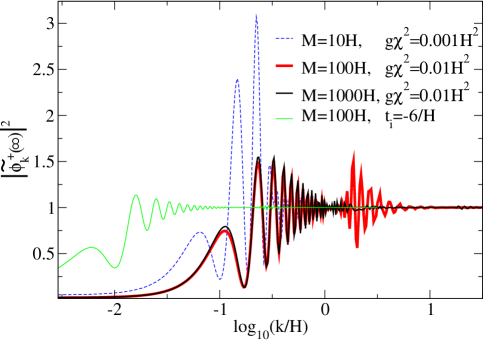
Figure 1: $|\tilde{\varphi}_{k}^{+}(\infty)|^{2}$ in units of $H^{2}$ for the hybrid inflation model, as a function of $\log_{10}(k/H)$ for several values of $M$ and $g\chi_{\rm he}^{2}$, rightmost three curves for $t_{0}=-4/H$. Leftmost curve shows the effect of taking an earlier initial time, $t_{0}=-6/H$, with $g\chi_{\rm he}^{2}=10^{-6}$.

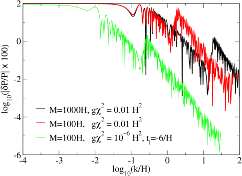
Figure 2: Log of absolute value of percent deviation of power spectrum as a function of $\log_{10}(k/H)$, for $M=100H$ and $M=1000H$, with $t_{0}=-4/H$ and $g\chi_{\rm he}^{2}=0.01H^{2}$, and $M=100H$ with $t_{0}=-6/H$ and $g\chi_{\rm he}^{2}=10^{-6}H^{2}$. Notice that the deviation is large at low $k$ not because the power is large, but rather because it is smaller than normal. Order of curves in legends coincides with that at right hand edge of the graph.

These figures show three main features, each of which has a simple physical explanation [9].

1. The fluctuation spectrum oscillates rapidly, due to the rapid driving by the fast $\chi$ oscillations.

2. The envelope of the oscillating inflaton fluctuations is strongly suppressed for the lowest $k$ values. This is because at early times the average value of $g\chi^{2}$ is potentially large, since $\langle\cos^{2}(Mt)\rangle={\textstyle{1\over 2}}$, and so the oscillating $\chi$ field behaves like an inflaton mass, and like a mass it suppresses fluctuations for small $k$. (It is because the CMB observations also appear to point to a similar suppression for small $k$, that these models provide a slight improvement in goodness-of-fit over fits to the standard concordance cosmology. The comparison of these models with the WMAP data is very similar to that given in ref. [12].)

3. The fluctuation spectrum rises to a peak, whose position is easily understood in terms of the driving frequency of the $\chi$ oscillations. These oscillations resonantly excite $\varphi$ modes having the same frequency, but the wavelength of these modes redshift as the universe expands. The peak occurs for wave-numbers corresponding to those modes which were driven at the earliest times, $t=t_{0}$, since this was the point when the driving $\chi$ field had the largest amplitude.

Detailed comparisons with the spectrum of CMB fluctuations show that an amplitude at horizon exit, $g\chi_{he}^{2}=10^{-5}H^{2}$ corresponds to a roughly 5% change in the CMB spectral parameters, making this a rough benchmark for how large an oscillation must be in order to have detectable effects. Given this benchmark, eq. (7) tells us how long before horizon exit inflation can have lasted without being overwhelmed by the energy in the damped $\chi$ oscillations. Pushing all parameters to make this time as long as possible leads in this model to $H\tau\mbox{\raisebox{-2.58334pt}{~{}$\stackrel{{\scriptstyle<}}{{\sim}}$~{}}}10$ $e$-foldings. A similar limit for $\tau$ is also obtained if one asks that the $\chi$ oscillations not lose all of their energy through decays into inflaton quanta. In other, less well motivated, models Ref. [9] a similar analysis shows heavy-field oscillations can have observable consequences for up to 30 $e$-foldings before horizon exit.

In summary, this model produces observable implications for the CMB because the fast motion of the background $\chi$-field makes the inflaton evolution non-adiabatic, and therefore causes positive- and negative-frequency modes to mix. Even outside of an inflationary context, nobody would expect to be able to describe the low-energy inflaton physics in the presence of these $\chi$ oscillations using an effective theory within which the $\chi$ field had been integrated out.

3 Adiabatic Physics

In this section we consider a model similar to the one examined above, but in which we make the more standard assumption that the background heavy fields do not oscillate. As a result the time evolution of the inflaton field is adiabatic, and the influence of the heavy fields is well described by a low-energy effective theory involving only the light degrees of freedom. For technical reasons we couch this section’s discussion in terms of a supersymmetric extension of the model just discussed. We use a supersymmetric model so that the heavy-field effective contributions to the inflaton potential do not destroy its flatness.

As is often the case with supersymmetric theories, in the model we consider the tree-level inflaton potential is exactly flat, but this flat direction is lifted by virtual loops of heavy particles. We show that the potential depends logarithmically on the heavy mass, leading to slow-roll parameters which are suppressed by factors of order $M_{0}^{2}/M^{2}$, where $M$ is the heavy mass but $M_{0}$ can be much larger than $H$. The model shows that heavy physics can decouple and yet still alter inflationary predictions for the CMB, since the figure of merit for deciding the observability of the heavy-physics effects can be larger than $H^{2}/M^{2}$.

3.1 The Model

Consider a globally-supersymmetric model containing the chiral multiplets, $\Phi=\{\phi,\psi\}$ and $H_{\pm}=\{h_{\pm},\chi_{\pm}\}$, coupled to a $U(1)$ gauge multiplet, $V=\{A_{\mu},\lambda\}$. $H_{+}$ and $H_{-}$ carry opposite $U(1)$ charges $\pm e$, and the multiplet $\Phi$ is neutral. The model’s superpotential and Kähler potential are

$$K=H_{+}^{*}H_{+}+H_{-}^{*}H_{-}+\Phi^{*}\Phi\qquad\hbox{and}\qquad W=g\Phi\,(H_{+}\,H_{-}-v^{2})\,,$$ (9)

where $g$ and $v$ are real constants. The associated scalar potential for this theory is $V=V_{F}+V_{D}$ where

$$V_{F} = g^{2}\left(\Bigl{|}h_{+}h_{-}-v^{2}\Bigr{|}^{2}+\Bigl{|}\phi\,h_{-}\Bigr{|}^{2}+\Bigl{|}\phi\,h_{+}\Bigr{|}^{2}\right)\,,$$

$$V_{D} = \frac{e^{2}}{2}\,\Bigl{(}|h_{+}|^{2}-|h_{-}|^{2}+\xi\Bigr{)}^{2}\,,$$ (10)

and $\xi>0$ is the Fayet-Iliopoulos term. The global minimum is supersymmetric with

$$\phi=0,\qquad|h_{\pm}|^{2}=\frac{1}{2}\Bigl{(}\mp\xi+\sqrt{\xi^{2}+4v^{4}}\Bigr{)}\,,$$ (11)

at which point $V=0$. There is a trough at $h_{\pm}=0$, for large $|\phi|$, along which $V_{\rm trough}(\phi)=V(h_{\pm}=0,\phi)=g^{2}\,v^{4}+{\textstyle{1\over 2}}\,e^{2}\xi^{2}$ is independent of $\phi$. The potential’s curvature in the $h_{\pm}$ directions is

$$M_{\pm}^{2}(\phi)=g^{2}|\phi|^{2}\pm\Delta\,,$$ (12)

with $\Delta=\sqrt{g^{4}v^{4}+e^{4}\xi^{2}}$, showing that the $h_{\pm}$ masses are positive for all $|\phi|^{2}>\Delta/g^{2}$, with masses which get bigger the larger $|\phi|$ is.

Along the trough’s bottom the gauge bosons are massless since the $U(1)$ gauge invariance is unbroken. The fermions $\lambda$ and $\psi$ are massless at tree level, while the fermions $\chi_{\pm}$ have masses

$$m^{2}_{\pm}(\phi)=m^{2}(\phi)=g^{2}|\phi|^{2}\,.$$ (13)

We therefore find a low-energy sector of strictly massless particles, $\{A_{\mu},\lambda,\phi,\psi\}$, which do not classically directly couple among themselves but which do couple to a massive sector, $\{h_{+},\chi_{+},h_{-},\chi_{-}\}$. Our interest is in the effective interactions which are generated amongst the light fields once these heavy modes are integrated out.

Integrating out the heavy fields leads to the following one-loop contribution to the low-energy scalar potential,

$$V_{\rm eff}(\phi) = \rho+\Delta V(\phi),$$ (14)

$$\hbox{with}\qquad\Delta V(\phi) = \delta\rho+\frac{2N}{64\pi^{2}}\sum_{i=\pm}\left[M_{i}^{4}(\phi)\,\ln\left({M_{i}^{2}(\phi)\over\mu^{2}}\right)-m_{i}^{4}(\phi)\,\ln\left({m_{i}^{2}(\phi)\over\mu^{2}}\right)\right]\,,$$

where $\rho=g^{2}\,v^{4}+{\textstyle{1\over 2}}\,e^{2}\xi^{2}$ is the renormalized (constant) classical potential along the trough, and $\delta\rho$ is the corresponding counter-term. (The overall factor of $N$ arises if we extend the model to include $N$ heavy multiplets, all sharing the same tree-level couplings to the light fields.) For $m^{2}(\phi)\gg\Delta$ this becomes

$$\Delta V_{\rm eff}(\phi)\approx\frac{N\,\Delta^{2}}{16\pi^{2}}\left[\ln\left({m^{2}(\phi)\over m_{*}^{2}}\right)+{\cal O}\left({\Delta^{2}\over m^{4}}\right)\right]\,,$$ (15)

where we adopt the renormalization condition that $\Delta V$ must vanish when $\phi=\phi_{*}$, defined as the field’s value at horizon exit. If $N_{e}$ $e$-foldings of inflation occur between horizon exit and the end of inflation, we have

$$m_{*}^{2}=m^{2}(\phi_{*})\approx m^{2}_{\rm end}+\frac{g^{2}NN_{e}\Delta^{2}}{12\pi^{2}H^{2}}\approx m^{2}_{\rm end}+\frac{g^{4}NN_{e}\,M_{p}^{2}}{4\pi^{2}},$$ (16)

where $m_{\rm end}^{2}$ is either $\Delta$ or $g^{4}NM_{p}^{2}/(8\pi^{2})$, whichever is larger. These estimates use the natural choice $e\sim g$ and $\xi\sim v^{2}$, for which $\Delta\sim g^{2}v^{2}$ and $\rho\sim g^{2}v^{4}$.

At horizon exit the inflationary parameters [13] which are predicted by this potential are

$$H^{2} = \frac{V}{3M_{p}^{2}}\approx\frac{\rho}{3M_{p}^{2}}\approx\frac{g^{2}v^{4}}{3M_{p}^{2}}\,,$$

$$\epsilon_{*} = \frac{1}{2}\left[{M_{p}\over V_{\rm eff}}\left({\partial V_{\rm eff}\over\partial\varphi}\right)\right]^{2}_{\varphi_{*}}\approx\frac{1}{2}\left[{M_{p}\,N\,\Delta^{2}\over 8\pi^{2}\rho\,\varphi_{*}}\right]^{2}\approx\left(\frac{g^{2}N}{32\pi^{2}N_{e}}\right)\,,$$

$$\eta_{*} = {M_{p}^{2}\over V_{\rm eff}}\left({\partial^{2}V_{\rm eff}\over\partial\varphi^{2}}\right)_{\varphi_{*}}\approx-\,{M_{p}^{2}\,N\,\Delta^{2}\over 8\pi^{2}\rho\,\varphi^{2}_{*}}\approx-\,\frac{1}{2N_{e}}\,,$$ (17)

where $\varphi=|\phi|$ is the inflaton. These equations shows that the roll is sufficiently slow if $\varphi/M_{p}\mbox{\raisebox{-2.58334pt}{~{}$\stackrel{{\scriptstyle>}}{{\sim}}$~{}}}g/4\pi$. Notice that if $\varphi$ should be as large as $O(M_{p})$ consistency would require us to embed this model into supergravity, a situation we can avoid if $g\ll 1$. For $N=1$ all of the requirements for inflation with $N_{e}\mbox{\raisebox{-2.58334pt}{~{}$\stackrel{{\scriptstyle>}}{{\sim}}$~{}}}60$ are satisfied — including fluctuation amplitudes which agree with CMB observations — if $v/M_{p}\sim g\sim 10^{-3}$.

For the purposes of comparing to decoupling arguments notice that the slow-roll parameters may be written

$$(2\epsilon_{*})^{1/2}\approx\frac{g^{2}N\Delta^{2}}{8\pi^{2}\,\rho}\,\left(\frac{\varphi_{*}\,M_{p}}{m^{2}_{*}}\right)\qquad\hbox{and}\qquad\eta_{*}\approx-\,\frac{g^{2}N\Delta^{2}}{8\pi^{2}\,\rho}\,\left(\frac{M_{p}^{2}}{m^{2}_{*}}\right)\,,$$ (18)

which implies the heavy physics decouples, inasmuch as both $\eta$ and $\epsilon$ are suppressed by inverse powers of the heavy mass, $m(\phi)$. But the scale against which $m^{2}(\phi)$ is compared is not $H^{2}$, but is instead either $(g^{4}N/8\pi^{2})M_{p}\,\varphi$ or $(g^{4}N/8\pi^{2})M_{p}^{2}$. (The condition $m(\phi)\ll M_{p}$ clearly again implies the coupling $g$ must be small.) If parameters are adjusted so that the heavy physics scale, $m_{*}$, is dialed to become larger and larger with $H$ fixed, then the slow roll parameters decrease, becoming closer and closer to the scale-invariant prediction $\epsilon_{*}=\eta_{*}=0$. This expresses the consequences of decoupling, since the entire inflaton potential is generated by virtual effects of the heavy physics. But because the benchmark for observability in this case is not $H^{2}/m^{2}_{*}$, the difference in their predictions can be kept observable even if $H^{2}/m_{*}^{2}$ is much smaller than a few percent.

In particular, imagine now comparing the effects for the CMB of two theories which differ only in that one has $N=1$ and the other has $N=2$ heavy sectors. If we suppose both models to undergo the same number of $e$-foldings of inflation, then they must also agree on their predictions for $\eta$. They can also predict identical fluctuation amplitudes so long as $v_{1}^{4}=v_{2}^{4}/2$, since $\delta\rho/\rho\propto H^{2}/(M_{p}^{2}\epsilon_{*})\propto(v/M_{p})^{4}(N_{e}/N)$. If they share the same couplings, $e\sim g$, then the models will predict $\epsilon_{*2}=2\epsilon_{*1}$, and so can have detectable differences in their predictions for CMB observables.

- [1] See, for example, David Spergel’s contributions to these proceedings for a recent summary of the WMAP observations.
- [2] D.N. Spergel et.al., [arXiv:astro-ph/0302209].
- [3] H.V. Peiris, et. al., [arXiv:astro-ph/0302225]; V. Barger, H.-S. Lee and D. Marfatia, [arXiv:hep-ph/0302150]; B. Kyae and Q. Shafi, [arXiv:astro-ph/0302504]; J.R. Ellis, M. Raidal and T. Yanagida, [arXiv:hep-ph/0303242].
- [4] J. Martin and R. H. Brandenberger, “The trans-Planckian problem of inflationary cosmology,” Phys. Rev. D 63, 123501 (2001) [arXiv:hep-th/0005209]; R. H. Brandenberger and J. Martin, “The robustness of inflation to changes in super-Planck-scale physics,” Mod. Phys. Lett. A 16, 999 (2001) [arXiv:astro-ph/0005432]; R. H. Brandenberger and J. Martin, “On the Dependence of the Spectra of Fluctuations in Inflationary Cosmology on Trans-Planckian Physics” [arXiv:hep-th/0305161].
- [5] R. Easther, B. R. Greene, W. H. Kinney and G. Shiu, “Inflation as a probe of short distance physics,” Phys. Rev. D 64, 103502 (2001) [arXiv:hep-th/0104102]; R. Easther, B. R. Greene, W. H. Kinney and G. Shiu, “Imprints of short distance physics on inflationary cosmology,” [arXiv:hep-th/0110226]; R. Easther, B. R. Greene, W. H. Kinney and G. Shiu, “A generic estimate of trans-Planckian modifications to the primordial power spectrum in inflation,” Phys. Rev. D 66, 023518 (2002) [arXiv:hep-th/0204129]; C. S. Chu, B. R. Greene and G. Shiu, “Remarks on inflation and noncommutative geometry,” Mod. Phys. Lett. A 16, 2231 (2001) [arXiv:hep-th/0011241]; J. Martin and R. H. Brandenberger, “A cosmological window on trans-Planckian physics,” [arXiv:astro-ph/0012031]; T. Tanaka, “A comment on trans-Planckian physics in inflationary universe,” [arXiv:astro-ph/0012431]; J. C. Niemeyer and R. Parentani, “Trans-Planckian dispersion and scale-invariance of inflationary perturbations,” Phys. Rev. D 64, 101301 (2001) [arXiv:astro-ph/0101451]; A. Kempf and J. C. Niemeyer, “Perturbation spectrum in inflation with cutoff,” Phys. Rev. D 64, 103501 (2001) [arXiv:astro-ph/0103225]; A. A. Starobinsky, “Robustness of the inflationary perturbation spectrum to trans-Planckian physics,” Pisma Zh. Eksp. Teor. Fiz. 73, 415 (2001) [JETP Lett. 73, 371 (2001)] [arXiv:astro-ph/0104043]; M. Bastero-Gil, “What can we learn by probing trans-Planckian physics,” [arXiv:hep-ph/0106133]; M. Lemoine, M. Lubo, J. Martin and J. P. Uzan, “The stress-energy tensor for trans-Planckian cosmology,” Phys. Rev. D 65, 023510 (2002) [arXiv:hep-th/0109128]; R. H. Brandenberger, S. E. Joras and J. Martin, “Trans-Planckian physics and the spectrum of fluctuations in a bouncing universe,” [arXiv:hep-th/0112122]; J. Martin and R. H. Brandenberger, “The Corley-Jacobson dispersion relation and trans-Planckian inflation,” Phys. Rev. D 65, 103514 (2002) [arXiv:hep-th/0201189]; G. Shiu and I. Wasserman, “On the signature of short distance scale in the cosmic microwave background,” Phys. Lett. B 536, 1 (2002) [arXiv:hep-th/0203113];
- [6] U. H. Danielsson, “A note on inflation and trans-Planckian physics,” Phys. Rev. D 66, 023511 (2002) [arXiv:hep-th/0203198]; S. F. Hassan and M. S. Sloth, “Trans-Planckian effects in inflationary cosmology and the modified uncertainty principle,” [arXiv:hep-th/0204110]; U. H. Danielsson, “Inflation, holography and the choice of vacuum in de Sitter space,” JHEP 0207, 040 (2002) [arXiv:hep-th/0205227]; A. A. Starobinsky and I. I. Tkachev, JETP Lett. 76, 235 (2002) [Pisma Zh. Eksp. Teor. Fiz. 76, 291 (2002)] [arXiv:astro-ph/0207572]; K. Goldstein and D. A. Lowe, “Initial state effects on the cosmic microwave background and trans-planckian physics,” [arXiv:hep-th/0208167]; U. H. Danielsson, “On the consistency of de Sitter vacua,” [arXiv:hep-th/0210058];
- [7] N. Kaloper, M. Kleban, A. Lawrence, S. Shenker, “Signatures of short distance physics in the cosmic microwave background”, [arXiv:hep-th/0201158]; N. Kaloper, M. Kleban, A. Lawrence, S. Shenker, and L. Susskind, “Initial conditions for inflation”, [arXiv:hep-th/0209231].
- [8] T. Banks and L. Mannelli, “De Sitter vacua, renormalization and locality”, Phys. Rev. D67 2003 065009, [arXiv:hep-th/0209113]; M. Einhorn and F. Larsen, “Interacting quantum field theory in de Sitter vacua”, Phys. Rev. D67 2003 024001, [arXiv:hep-th/0209159]; M. Einhorn and F. Larsen, “Squeezed States in the de Sitter Vacuum”, [arXiv: hep-th/0305056]; K. Goldstein and D. A. Lowe, “A note on alpha-vacua and interacting field theory in de Sitter space” ,[arXiv: hep-th/0302050]. Hael Collins, R. Holman and Matthew R. Martin, “The Fate of the -Vacuum”, [arXiv:hep-th/0306028].
- [9] C.P. Burgess, J.M. Cline, F. Lemieux and R. Holman, “Are Inflationary Predictions Sensitive to Very High Energy Physics?” [arXiv: hep-th/0210233].
- [10] C.P Burgess, J.M. Cline and R. Holman, “Effective Field Theories and Inflation” [arXiv: hep-th/0306079].
- [11] A. Linde, “Hybrid inflation”, Phys. Rev. D 49 (1994) 748 [arXiv:astro-ph/9307002]; David H. Lyth and Ewan Stewart,“ More varieties of hybrid inflation”, Phys. Rev. D54 (1996) 7186, [arXiv:hep-ph/9606412].
- [12] J. M. Cline, P. Crotty and J. Lesgourgues, “Does the small CMB quadrupole moment suggest new physics?,” arXiv:astro-ph/0304558.
- [13] Andrew R. Liddle and David H. Lyth “Cosmological Inflation and Large Scale Structure”, Cambridge University Press (2000).
- [14] For a review with references see D.H. Lyth and A. Riotto, “Particle Physics Models of Inflation and the Cosmological Density Perturbation”, Phys. Rep. C 3141(1999).
- [15] P. Binetruy and G.R. Dvali, Phys. Lett. B388 (1996) 241-246, [arXiv:hep-ph/9606342]; E. Halyo, Phys. Lett. B387 (1996) 43-47 [arXiv:hep-ph/9606423]; C. Panagiotakopoulos, Phys. Rev. D55 (1997) 7335-7339 [arXiv:hep-ph/9702433]; Phys. Lett. B402 (1997) 257-262 [arXiv:hep-ph/9703443]; A.D. Linde and A. Riotto, Phys. Rev. D56 (1997) 1841–1844 [arXiv:hep-ph/9703209]; L. Covi, G. Mangano, A. Masiero and G. Miele, Phys. Lett. B424 (1998) 253-258 [arXiv:hep-ph/9707405]; M. Bastero-Gil and S. F. King, Phys. Lett. B423 (1998) 27 [arXiv:astro-ph/9709502]; G.R. Dvali, G. Lazarides and Q. Shafi, Phys. Lett. B424 (1998) 259-264 [arXiv:hep-ph/9710314].