The line–of–sight distribution of the gas in the inner 60 pc of the Galaxy

2MASS K_S band data of the inner 60 pc of the Galaxy are used to reconstruct the line-of-sight distances of the giant molecular clouds located in this region. Using the 2MASS H band image of the same region, two different populations of point sources are identified according to their flux ratio in the two bands. The population of blue point sources forms a homogeneous foreground that has to be subtracted before analyzing the K_S band image. The reconstruction is made using two basic assumptions: (i) an axis-symmetric stellar distribution in the region of interest and (ii) optically thick clouds with an area filling factor of $\sim$1 that block all light of stars located behind them. Due to the reconstruction method, the relative distance between the different cloud complexes is a robust result, whereas it is not excluded that the absolute distance with respect to Sgr A^∗ of structures located more than 10 pc in front of Sgr A^∗ are understimated by up to a factor of 2. It is shown that all structures observed in the 1.2 mm continuum and in the CS(2-1) line are present in absorption. We place the 50 km s^-1 cloud complex close to, but in front of, Sgr A^∗. The 20 km s^-1 cloud complex is located in front of the 50 km s^-1 cloud complex and has a large LOS distance gradient along the direction of the galactic longitude. The bulk of the Circumnuclear Disk is not seen in absorption. This leads to an upper limit of the cloud sizes within the Circumnuclear Disk of $\sim$0.06 pc.

1 Introduction

The Galactic Center (GC) is a unique place to study the fueling of a central black hole in great detail. The black hole, which coincides with the non-thermal radio continuum source Sgr A^∗, has a mass of $\sim$3 10⁶ M_⊙ (Eckart & Genzel 1996). At a distance between 2 pc and 7 pc a ring-like structure made of distinct clumps, which is called the Circumnuclear Disk (CND) is rotating around the central point mass. The inner ionized edge of the CND is a part of a structure of ionized gas (see e.g. Lo & Claussen 1983, Lacy et al. 1991) that resembles a spiral and is therefore called the Minispiral. Sgr A^∗ is surrounded by a huge Hii region Sgr A West with a size of 2.1$\times$2.9 pc, which was first observed by Ekers et al. (1975).

The Circumnuclear disk has been observed in several molecular lines: Gatley et al. (1986) (H₂), Serabyn et al. (1986) (CO,CS), Güsten et al. (1987) (HCN), DePoy et al. (1989) (H₂), Sutton et al. (1990) (CO), Jackson et al. (1993) (HCN), Marr et al. (1993) (HCN), Coil & Ho (1999, 2000) (NH₃), and Wright et al. (2001) (HCN). The deduced properties of the CND are the following: it has a mass of a few 10⁴ M_⊙; the ring is very clumpy with an estimated volume filling factor of $\Phi_{\rm V}\sim 0.01$ and an area filling factor of $\Phi_{\rm A}\sim 0.1$; the clumps have masses of $\sim$30 M_⊙, sizes of $\leq$0.1 pc, and temperatures $\geq$100 K.

These observations together with mm continuum observations (see, e.g. Mezger et al. 1989, Dent et al. 1993) have shown that three giant molecular clouds (GMCs) are located in the inner 60 pc of the Galactic Center. Following Zylka et al. (1990) these are: (i) Sgr A East Core, a compact giant molecular cloud with a gas mass of several 10⁵ M_⊙ that is located to the north–east of Sgr A^∗. (ii) The giant molecular cloud M-0.02-0.07 that is located to the east of Sgr A^∗. Since its main radial velocity is $\sim$50 km s^-1, it is also called the 50 km s^-1 cloud. (iii) The GMC complex M-0.13-0.08 that is located to the south of Sgr A^∗. Since its main radial velocity is $\sim$20 km s^-1, it is also called the 20 km s^-1 cloud. Coil & Ho (1999, 2000), and Wright et al. (2001) argue that there are physical connections between these GMC complexes and the CND on the grounds of radial velocities, projected distances, and linewidths. Their analysis misses crucial information, i.e. the gas distribution in the line–of–sight (LOS). With this information it is possible to place the GMC complexes in three–dimensional space and confirm or exclude possible connections with the CND.

In this article we use 2MASS near infrared data that show the GMC complexes in absorption to reconstruct the LOS distribution of the gas in the inner 60 pc of the Galactic Center. We use the absorption features in the NIR continuum emission whose level over a large scale ($\sim 13^{\prime}$) is very difficult to obtain.

This article has the following structure: the 2MASS data are presented in Sect. 2 followed by the description of the data reduction (Sect. 3). The final K_S band images are presented in Sect. 4. We explain the method of the reconstruction of the line-of-sight distances and show its results in Sect. 5. The reconstructed line-of-sight distribution is discussed and compared to mm observations in Sect. 6. We give our conclusions in Sect. 7.

2 The data

We use the near–infrared (NIR) data of the Two Micron All Sky Survey (2MASS). Six uncompressed full–resolution Atlas images in J (1.25 $\mu$m), H (1.65 $\mu$m), and K_S (2.17 $\mu$m) covering the inner $30^{\prime}\times 20^{\prime}$ of the Galactic Center (Fig. 1) were downloaded via the 2MASS Batch Image Server on the IRSA site. Single images have sizes of 512$\times$1024 pixels. Each pixel has a size of $1^{\prime\prime}$. The images are overlapping over a region of 53 pixels in declination and 89 pixels in right ascension. The effective resolution of these observations was $\sim 3^{\prime\prime}$.

3 Data reduction

3.1 NIR continuum

All images were analyzed using the MOPSI software. Since we are interested in the stellar continuum, all 6 images had to be put together properly with special care taken for the sky and system emission correction. We used the inner image, which includes the Galactic Center, as the reference image. Fig. 1 shows the configuration of the 6 2MASS images in the sky.

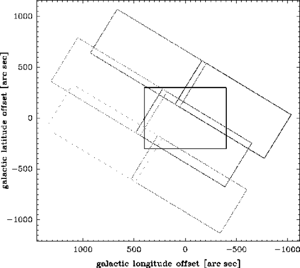
Figure 1: Mosaic of 2MASS images centered on Sgr A^∗. The thick box delineates our region of interest.

In a first step the constant offset between the reference image and a second, neighbouring image was calculated. It turned out that these zero order corrections gave unsatisfactory results. Therefore, we used the overlapping region to correct the neighbouring image for a constant tilt. All 5 surrounding images were treated in this way, in order to ensure smooth transitions between the images and thus flat baselines for the stellar continuum emission. At the end an image of $800^{\prime\prime}\times 600^{\prime\prime}$ centered on Sgr A^∗ was used.

3.2 Single stars

The images in all wavelengths contain foreground stars to different extents. Following Launhardt et al. (2002) we divide the foreground star populations into 4 classes: (i) Galactic Disk stars, (ii) Galactic Bulge stars, (iii) Nuclear Stellar Disk, and (iv) Nuclear Stellar Cluster stars. The Nuclear Stellar Disk and the Nuclear Stellar Cluster form the Nuclear Bulge. The dereddend COBE fluxes at 2.2 $\mu$m (with a resolution of 0.7${}^{\rm o}\simeq$ 100 pc) of the Galactic and the Nuclear Bulge are of the same order, whereas the emission of the Galactic Disk is negligible (Launhardt et al. 2002). Philipp et al. (1999) estimated that more than 80% of the integrated flux density of the inner 30 pc is contributed by stars located in the Nuclear Bulge.

The overall populations of low and intermediate-mass main sequence stars in the Nuclear and Galactic Bulge are similar, but the central 30 pc have an overabundance of K-luminous giants. These giants are more concentrated towards the center than low-mass main sequence stars (Philipp et al. 1999). The near infrared luminosity of the central 30 pc is dominated by these evolved stars, whose contribution to the total stellar mass is however negligible (Mezger et al. 1999).

Launhardt et al. (2002) estimate the extinction due to interstellar dust in the Galactic Disk/Bulge and due to the Nuclear Bulge to be of the same order ($A_{\rm V}=15$ mag). The total extinction to the Galactic Center is thus $A_{\rm V}=30$ mag. Due to the $\lambda^{2}$ law of the dust opacity, the stars in the Nuclear Bulge are fainter in the J and H band. Thus, these bands are more contaminated by Galactic Bulge stars than the K_S band. This can be qualitatively seen in Fig. 2 that shows a cut along Galactic longitude through Sgr A^∗. The central stellar cluster, which is most prominent in the K_S band, is more and more buried in the continuum due to foreground stars in the J and H band.

Figure 2: Slice of the 2MASS images through Sgr A^∗ parallel to the galactic longitude. Solid line: K_S band. Dashed line: H band. Dotted line: J band.

Since we are only interested in the stellar distribution of the Nuclear Bulge, we only use the K_S band image and the K_S–H color for our studies.

In both bands, K_S and H, single, distinguishable point sources are visible. The point spread function of the 2MASS data does not have the shape of the seeing-determined point spread function and is difficult to approximate by an analytic formula. We use a modified Lorentzian profile to fit and subtract the distinct point sources. The usage and advantages of a modified Lorentzian profile are described in Philipp et al. (1999). Fig. 3 shows an example of a small field before and after subtracting the point sources.

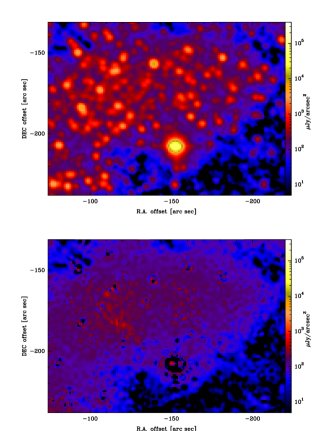
Figure 3: Upper panel: a subfield of the original K_S band image. Lower panel: same image after subtraction of Lorentzian fits to the point sources. The offsets are given with respect to Sgr A^∗.

Since the effective resolution of 3^′′ is not sufficient to resolve all stars, there are often several in projection closely packed stars that appear as a point source in the 2MASS image. In order to illustrate this effect, we show in Fig. 4 a small area $\sim$5 pc north-east of Sgr A^∗ of the 2MASS image together with an image of the same region observed with IRAC2B (Philipp et al. 1999).

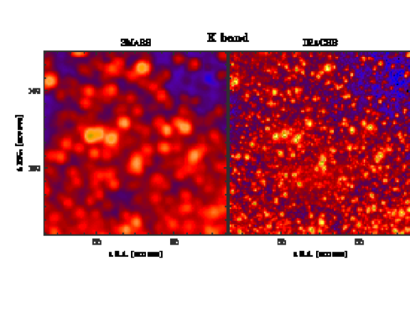
Figure 4: K_S band images of a small subfield $\sim$5 pc north-east from Sgr A^∗. Left panel: 2MASS image with 3^′′ effective resolution. Right panel: IRAC2B image with 1^′′ resolution (Philipp et al. 1999). The coordinates are offsets with respect to Sgr A^∗.

The IRAC2B image has a seeing of of $\sim$1^′′. Clearly, several point sources in the 2MASS image are resolved into multiple point sources in the IRAC2B image. This effect complicates the shape of the 2MASS point source profiles and makes a subtraction difficult. Our point source detection limit is $\sim$0.3 mJy, the completeness limit is $\sim$3 mJy in the K_S band. In this way we found $\sim$75 000 point sources in the whole field and $\sim$13 500 point sources in our region of interest (see Fig. 1).

For the color determination we sum the flux of all point sources in a circle of 3^′′ (the seeing) diameter around the positions of a given point source in the K_S band. In a second step, we sum the flux of all point sources in the H band within a circle of the same diameter. This proved to be the best method for an accurate correlation of a sufficient number of point sources in both bands. In this way we find $\sim$60 000 point sources in both bands in the whole field and $\sim$12 000 point sources in our region of interest (see Fig. 1). Fig. 5 shows the K_S/H flux ratio distribution of the point sources as a function of their distance to Sgr A^∗ (upper panel) and the K_S/H flux ratio distribution as a function of the K_S band flux (middle panel).

Figure 5: Upper panel: K_S/H flux ratio distribution of the point sources as a function of their distance to Sgr A^∗. Middle panel: K_S/H flux ratio distribution as a function of the K_S band flux. Lower panel: theoretical K_S/H flux ratio for stars with different effective temperatures. Solid line: no reddening. Dashed line: reddening corresponding to $A_{\rm V}$=15 mag. Dotted line: reddening corresponding to $A_{\rm V}$=30 mag.

The point sources clearly become redder towards the Galactic Center. The trend that faint sources are bluer is due to our way of finding correlated point sources and is not a physical effect. In order to discriminate between the stars in the Nuclear Stellar Disk and the Nuclear Stellar Cluster, we use a limiting K_S/H flux ratio of 4, which is represented as a horizontal line in Fig. 5. This limit is chosen in a way to assign the majority of the stars to the Nuclear Stellar Disk. The remaining stars belong with a high probability to the Nuclear Stellar Cluster.

Fig. 6 shows the radial distribution of the K_S band flux of the blue point sources averaged over ellipsoids with an axis ratio of 1.4:1, which is consistent with the K_S isocontours of the Nuclear Bulge.

Figure 6: Radial profile of the blue point sources averaged over ellipsoids with an axis ratio of 1.4:1.

From 100^′′ to 300^′′ the radial distribution is almost flat and has a value of $\sim$300 $\mu$Jy. The standard deviation increases with decreasing radius, because of the decreasing area of the rings of integration near the center. The inner maximum is mainly due to one luminous point source, which is the central cluster of Hei stars. There is also a slight increase of the mean integrated flux density to the center to a value of $\sim$400 $\mu$Jy. Since the K_S band intensity reaches maximum values of $\sim$10 mJy the radial profile can be regarded as constant even for small radii. We conclude that the blue point sources represent an almost homogeneous foreground distribution that can be removed without changing the distribution of the Nuclear Stellar Cluster.

With our K_S band completeness limit of $\sim$3 mJy we can observe hot main sequence stars, cold giants, hot and cold supergiants, and Wolf-Rayet stars as distinguishable point sources (see Fig. D1 of Philipp et al. 1999). The lower panel of Fig. 5 shows the theoretically expected K_S/H band flux ratios for stars with a given effective temperature (i) without reddening, (ii) with a reddening corresponding to $A_{\rm V}$=15 mag (Galactic Disk/Bulge), and (iii) with a reddening corresponding to $A_{\rm V}$=30 mag (Galactic Disk/Bulge and Nuclear Bulge). We use the dust opacities of Launhardt et al. (2002) and $A_{\rm V}/N_{\rm H}=3.25\,10^{-22}$, which is a factor $\sim$1.6 lower than the value given by the same authors. With a total reddening of $A_{\rm V}$=30 mag and a limiting K_S/H flux ratio of 4 we theoretically expect to find mainly supergiants of temperatures smaller than 30 000 K. The fact that we classify the central Hei star cluster as a blue point source justifies a posteriori the $A_{\rm V}/N_{\rm H}$ we use.

Fig. 7 shows the radial distribution of the K_S band flux of the red point sources averaged over the same ellipsoids.

Figure 7: Solid line: radial profile of the red point sources averaged over ellipsoids with an axis ratio of 1.4:1. Dashed line: Slice parallel to the galactic longitude through Sgr A^∗ through the K_S image where all point sources (red and blue) are subtracted.

The flux of this stellar population is dominated by sources of flux densities between 10 and 100 mJy. Its radial profile is markedly different from that of the blue point sources. It rises steeply in the inner 50^′′ from 500 $\mu$Jy to 10 mJy in the center. For $R>20^{\prime\prime}$ the flux density of the red point sources represents only a small fraction ($<20$%) of the flux density of the unresolved background (Fig. 7). Thus, the red point sources represent Central Stellar Disk stars, which justifies our limiting K_S/H flux ratio.

The total flux density of the blue point sources is 155 Jy, that of the red point sources 110 Jy. We find a flux density of the background of 335 Jy. Philipp et al. (1999) analyzed K band data of a $10^{\prime}\times 10^{\prime}$ field centered on Sgr A^∗. They found a total K band flux of 752 Jy and a total stellar flux density of 370 Jy and estimated the flux of the background to be 283 Jy. Their total flux density (blue and red sources included) is 25% higher than that of the 2MASS image ($S$=600 Jy). The fraction of the flux density of fitted point sources to the total flux density is 0.44 for the 2MASS data and 0.49 for the data of Philipp et al. (1999). Thus, we conclude that our fitting procedure works in a satisfactory way.

In the end we made two different images:

1. an image where only the blue foreground point sources are subtracted,

2. an image where all point sources that could be identified are subtracted.

4 Results

In the inner 100 pc of the Galaxy the gas is highly clumped in giant molecular clouds with a volume filling factor of $\sim$1% (Launhardt 2002). Following Zylka et al. (1990) three main giant molecular cloud complexes can be distinguished: (i) Sgr A East Core, (ii) the $\sim$50 km s^-1 cloud, and (iii) the 20 km s^-1 cloud. Sgr East core is part of the 50 km s^-1 cloud complex, thus we will treat these features as a single structure. Fig. 8 shows a sketch of the projected inner 30 pc of the Galaxy, where the main features are indicated (Minispiral, CND, 20 km s^-1 cloud, 50 km s^-1 cloud).

Figure 8: Sketch of the inner 30 pc of the Galaxy. The central black dot represents the Hei star cluster surrounded by the Minispiral and the CND (where only the high velocity lobes are shown). The 20 and 50 km s^-1 giant molecular clouds are located at negative latitudes. Capital letters indicate structures discussed in the text. 1 pc corresponds to 24^′′.

Fig. 9 shows the K_S band image of the Galactic Center region (i) with only the blue point sources subtracted, (ii) with all distinguishable point sources subtracted.

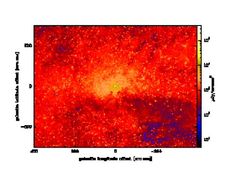
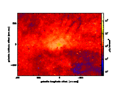
Figure 9: K_S band image of the Galactic Center region. Upper panel: only the blue point sources are subtracted. Lower panel: all distinguishable point sources are subtracted.

In both images the absorption features are very similar. This shows again that the foreground stars, despite their extended wings of their profiles, do not affect considerably the underlying continuum emission. Thus, the image where all point sources (blue and red) are subtracted has a less discrete character, i.e. it is less noisy.

In the inner $10^{\prime\prime}$ around Sgr A^∗, i.e. in the very central star cluster, the procedure of point source subtraction is not reliable. It mainly subtracted the central peak. Thus, this region has to be discarded in the discussion using the image where all point sources are subtracted. In the following we will discuss the main features of both images, because of their similarity.

One clearly can distinguish the 20 km s^-1 and the 50 km s^-1 cloud complexes at negative galactic latitudes (see Fig. 8). The 20 km s^-1 cloud complex has an almost linear edge to positive galactic latitudes. It covers a region of nearly 7^′ in galactic longitude. The depth of the absorption is almost constant from $\Delta l\sim-80^{\prime\prime}$ to $\Delta l\sim-400^{\prime\prime}$ with respect to Sgr A^∗. The 50 km s^-1 cloud complex is separated into two components. The first, located below Sgr A^∗ at negative galactic latitudes, is curved. The second component runs almost perpendicular to the first at a galactic longitude of $\Delta l\sim 200^{\prime\prime}$ with respect to Sgr A^∗ (D in Fig. 8). Whereas the absorption caused by the first component is almost uniform, the second component shows a gradient. The absorption depth of the first component is smaller than that of the 20 km s^-1 cloud complex.

Furthermore, there is a large cloud complex at $\Delta l\sim-200^{\prime\prime}$, $\Delta b\sim-250^{\prime\prime}$ that forms a shell-like structure (A in Fig. 8). The part towards Sgr A^∗ has a larger absorption depth than the opposite side.

At positive galactic latitudes one can find two further absorption features. One at positive galactic longitudes that appears to be elongated diagonal to the image axis (C in Fig. 8). The second one at negative galactic longitudes has the shape of the letter U (B in Fig. 8). We believe that this is a foreground cloud and we will not discuss it further.

It is important to note that there is almost no absorption along the galactic plane and little absorption for positive galactic latitudes at $\Delta l=0$ with respect to Sgr A^∗.

5 Reconstruction of the LOS distribution

In this Section we describe the method to calculate the distance along the line–of–sight (LOS) of the molecular cloud complexes observed in K_S band absorption. We model the K_S band continuum emission distribution using analytical expressions for the stellar volume emissivity. We use the image where all point sources are subtracted, but we also apply the method to the image where only the red point sources are subtracted to make sure that the subtraction of the red point sources does not alter the results.

For the reconstruction we make three basic assumptions:

1. We assume an axis–symmetric distribution of stars in the central 7^′ around Sgr A^∗.

2. We assume that the clouds are optically thick and that their area coverage factor is $\sim$1. This means that the clouds block the light of all stars located behind them. The average column density of the inner 100 pc of the Galaxy is $\sim$7 10²² cm^-2 (Launhardt et al. 2002). Assuming an area filling factor of 10% the mean density is 10⁴ cm^-3, which is about the critical density to resist tidal shear (Vollmer & Duschl 2001). Thus the column density of a giant molecular cloud is $\sim$7 10²³ cm^-2 leading to a K band extinction of $A_{\rm K}\sim 28$ mag (using $A_{\rm K}/A_{\rm V}=0.122$, Mathis et al. 1983).

3. We assume a homogeneous large scale reddening gas layer within the Nuclear Bulge in front of the GMCs, which is due to the pervasive, low density phase of the ISM. For a field twice as large as our region of interest, we observe a variation in the large scale reddening.

5.1 The method

We first fit an analytic profile to the volume emissivity of the central stellar distribution in the inner 60 pc around Sgr A^∗. Following Launhardt et al. (2002) we use two components: (i) the Nuclear Stellar Cluster at $R<1$ pc and (ii) the Nuclear Stellar Disk for radii $R<100$ pc around Sgr A^∗. We use the following analytic expressions:

$$({\rm i})\ \ \rho_{1}(x,y,z)=\frac{\rho_{0}}{1+(\frac{x}{r_{0}})^{2}+(\frac{y}{r_{1}})^{2}+(\frac{z}{r_{0}})^{2}}\ ,$$ (1)

$$({\rm ii})\ \ \rho_{2}(x,y,z)=\frac{\rho_{1}}{\sqrt{(\frac{x}{r_{2}})^{2}+(\frac{z}{r_{2}})^{2}}}\times{\rm sech}^{2}\big{(}\frac{y}{y_{0}}\big{)}\ ,\ {\rm and\ alternatively}$$ (2)

$$\ \ \ \ \ \ \rho_{2}(x,y,z)=\tilde{\rho}_{1}\,\exp\big{(}{\rm ln}(\frac{1}{2})|R/c|\big{)}\times{\rm sech}^{2}\big{(}\frac{y}{y_{0}}\big{)}\ ,$$ (3)

where $x$/$y$ are the distances along the galactic longitude/latitude, $z$ is the distance along the LOS with respect to Sgr A^∗, $R=\sqrt{x^{2}+y^{2}+z^{2}}$, $\rho_{0}/\rho_{1}=5\,10^{3}$, $\rho_{0}/\tilde{\rho}_{1}=6.6\,10^{4}$, $r_{0}$=0.1 pc, $r_{1}$=0.07 pc, $r_{2}$=1 pc, $y_{0}$=10 pc, and $c$=120 pc. The profile of Eq. (3) was designed to fit the COBE data of 0.7^o resolution (Launhardt et al. 2002). Since a constant radial density is dynamically difficult to explain, we give an alternative profile of the form $\rho_{2}\propto R^{-1}$ (Eq. (2)). The total volume emissivity is $\rho(x,y,z)=\rho_{1}(x,y,z)+\rho_{2}(x,y,z)$ in model units.

The volume emissivity is integrated along the LOS. As a next step a constant offset is subtracted from the K_S band data to account for homogeneous foreground emission. Then, the model map is multiplied by a factor $\xi$ to fit the K_S band image. This factor is found in minimizing the difference between the model and the observed data. The result of this procedure can be seen in Fig. 10, where slices of the resulting model intensity along the galactic longitude and latitude through Sgr A^∗ together with slices of the K_S data are shown.

Figure 10: Slices of the model intensities along the galactic longitude and latitude through Sgr A^∗ together with slices of the K_S data. Dotted line: Eq. (2)/(4) $a=0$, $z_{0}=$-50 pc. Dashed line: Eq. (2)/(4) $a=0$, $z_{0}=-100$ pc. Dash-dotted line: Eq. (3)/(4) $a=0$. 1 pc corresponds to 24^′′.

The model slices of Eq. (2) nicely fit the data in the regions without absorption. Since the model distribution along the Galactic latitude has the same form for Eq. (2) and Eq. (3), it fits equally well the observed K_S band emission distribution. The emission distribution along the Galactic Longitude is overestimated by Eq. (3). We conclude that Eq. (2) fits the data better.

We define

$$I_{0}(x,y)=\xi\int^{z_{1}}_{z_{0}}\rho(x,y,\tilde{z}){\rm d}\tilde{z}\ ,$$ (4)

$$I_{z}(x,y)=\xi\int^{z}_{z_{0}}\rho(x,y,\tilde{z}){\rm d}\tilde{z}\ .$$ (5)

where the lower boundary $z_{0}$ is negative and fixed and $z_{1}=|z_{0}|$. Let $I_{\rm K}(x,y)$ be the K_S band intensity. Then, the LOS distance $z$ for a given position $(x,y)$ is given by

$$\frac{I_{z}(x,y)}{I_{0}(x,y)}=\frac{I_{\rm K}(x,y)}{I_{0}(x,y)}\ ,$$ (6)

or

$$I_{z}(x,y)=I_{\rm K}(x,y)\ .$$ (7)

Since the intensity of sky is not known, we will generalize our method in subtracting a constant intensity $a$ from the image. The sky intensity of Fig. 9 is determined by assuming that the darkest region in the whole field (cf. Fig. 1) has zero intensity. Thus, the equation for the determination of the LOS distance of gas located at ($x$, $y$) yields:

$$I_{\rm K}(x,y)-a=\xi I_{z}(x,y)\ ,$$ (8)

In order to investigate how $z$ varies with $\xi$ and $a$ we set

$$I_{z}(x,y)=\int_{z_{0}}^{z}\rho_{1}(x,y,\tilde{z}){\rm d}\tilde{z}=\xi^{-1}(I_{\rm K}(x,y)-a)\ .$$ (9)

Solving this equation for $z$ yields

$$\tilde{z}=(1+x^{2}+y^{2})\tan\big{(}(1+x^{2}+y^{2})(\rho_{0}^{-1}(\xi^{-1}(I_{\rm K}(x,y)-a)))-\frac{\pi}{2}\big{)}\ .$$ (10)

thus, small variations in $I_{\rm K}(x,y)$ lead to large variations in $z$ for large projected distances and small $I_{\rm K}(x,y)$, i.e. large LOS distances $z$.

In order to illustrate this effect for the realistic volume emissivity $\rho=\rho_{1}+\rho_{2}$, we show $z$ as a function of $I_{z}/I_{0}$ for 3 different projected distances in Fig. 11.

Figure 11: LOS distance $z$ as a function of the ratio $I_{z}/I_{0}$ for 3 different projected distances: Solid line: (2 pc, 0.5 pc), dashed line: (5 pc, 5 pc), dot-dashed line: (10 pc, 5 pc).

For deep absorption features small variations in $I_{z}/I_{0}$ lead to large variations in $\tilde{z}$. The non-linear regime begins at smaller LOS distances for large projected distances. The error of the LOS distance for large projected and LOS distances can be of the order of $\sim$30%.

Due to the radial distribution of the volume emissivity, this method detects easily clouds in front of Sgr A^∗. Clouds that are located behind Sgr A^∗ show only small absorption features that can be buried by the discrete character of the signal (single stars).

Clearly, the LOS distance depends strongly on the offset $a$ (Eq. (8)) applied on the data. There is no way to determine a priori this constant. In addition, due to the form of $\rho_{2}$ in Eq. (2) the LOS distance depends on $z_{0}$.

We made 4 different calculations for the profile of Eq. (refeq:alt1) and 2 calculations for the profile of Eq. (3) to take these effects into account. For Eq. (2) we set:

1. $z_{0}$=-50 pc, $a$=0;

2. $z_{0}$=-50 pc, $a$=150 $\mu$Jy/arcsec²;

3. $z_{0}$=-100 pc, $a$=0;

4. $z_{0}$=-100 pc, $a$=150 $\mu$Jy/arcsec²;

for Eq. (3) we set:

1. $z_{0}$=-150 pc, $a$=0;

2. $z_{0}$=-150 pc, $a$=150 $\mu$Jy/arcsec².

Since the profile of Eq. (3) has a cutoff at $R$=120 pc, it is not necessary to vary the the lower integration limit $z_{0}$ of Eq. (4).

The value of the offset $a$ is chosen such that the deepest absorption at $\Delta l\sim-200^{\prime\prime}$, $\Delta b\sim-200^{\prime\prime}$, which most probably belongs to the 20 km s^-1 cloud complex, is close to zero (cf. Sect. 5.2). For comparison, Launhardt et al. (2002) estimate the K band flux of the Galactic Disk and Bulge to be $\sim$20 MJy/sr=470$\mu$Jy/arcsec² and that of the COBE peak emission of the Nuclear Bulge to be $\sim$10 MJy/sr=235$\mu$Jy/arcsec². This implies that cloud A (Fig. 8) is located within the Nuclear Bulge.

5.2 Results

In order to demonstrate the differences between the 4 different reconstructions using Eq. (2), we show in Fig. 12 a slice through the reconstructed map at $\Delta b=-70^{\prime\prime}$ parallel to the galactic longitude. This is a representative cut through the 50 and 20 km s^-1 cloud complexes. For clarity we applied a median filter with a size of 11 pixels to the map. Negative distances are in front Sgr A^∗.

Figure 12: Reconstruction of the LOS distances for a slice at $\Delta b=-70^{\prime\prime}$ parallel to the galactic longitude using Eq. (2). Solid line: $a$=150 $\mu$Jy/arcsec² and $z_{0}=-50$ pc. Dotted line: $a$=0 $z_{0}=-50$ pc. Dashed line: $a$=150 $\mu$Jy/arcsec² and $z_{0}=-100$ pc. Dot-dashed line: $a$=0 $z_{0}=-100$ pc. Negative distances are in front of Sgr A^∗.

As expected, the larger $|z_{0}|$ and $a$ the smaller is the LOS distance of the clouds, i.e. the nearer it is to the observer. For the deepest absorption at $\Delta l=-100^{\prime\prime}$ the LOS distance is $d\sim-60$ pc for $z_{0}=-100$ pc, $a$=150 $\mu$Jy/arcsec² and only $d\sim-17$ pc for $z_{0}=-50$ pc, $a$=0. With increasing $z_{0}$ and $a$ the variation of the LOS distance within the 20 km s^-1 increases rapidly. On the other hand, the LOS distance of the 50 km s^-1 cloud complex ($0^{\prime\prime}<\Delta l<200^{\prime\prime}$) does not vary much with varying $z_{0}$ and $a$, because it is located very close to Sgr A^∗ (0 pc$<d<-5$ pc).

Fig. 13 shows the 2 different reconstructions using Eq. (3).

Figure 13: Reconstruction of the LOS distances for a slice at $\Delta b=-70^{\prime\prime}$ parallel to the galactic longitude using Eq. (3). Solid line: $a$=0 and $z_{0}=-150$ pc. Dashed line: $a$=150 $\mu$Jy/arcsec² and $z_{0}=-150$ pc. Negative distances are in front of Sgr A^∗.

The LOS distances of the 50 km s^-1 cloud complex are comparable to those calculated using Eq. (2). However, the LOS distances from Sgr A^∗ of the 20 km s^-1 cloud complex are systematically larger than those calculated using Eq. (2). This is due to the too high model continuum with respect to the K_S band continuum emission (Fig. 10). The relative distances between the molecular cloud complexes and the relative gradients of the LOS distance within a cloud complex are the same for both model profiles.

We chose a profile using Eq. (2) with $z_{0}=-50$ pc and $a$=150 $\mu$Jy/arcsec² for the final reconstruction of the LOS distance distribution. This represents a compromise between a possible underestimation of the LOS distances due to an offset in the K_S band data and too much variation of the LOS distances within the 20 km s^-1 cloud complex. One has to bear in mind that LOS distances $d>-10$ pc have a small error, whereas distances $d<-10$ pc can be up to a factor of 2 smaller than given in the final map.

Fig. 14 shows the map of the reconstructed LOS distances for the 2MASS K_S images with $z_{0}=-50$ pc and $a$=150 $\mu$Jy/arcsec² for two cases: (i) all blue point sources are subtracted and (ii) all point sources (blue and red) are subtracted.

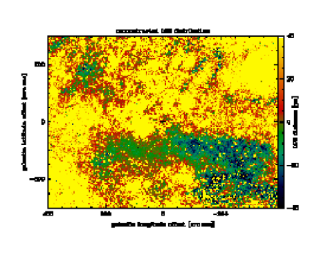
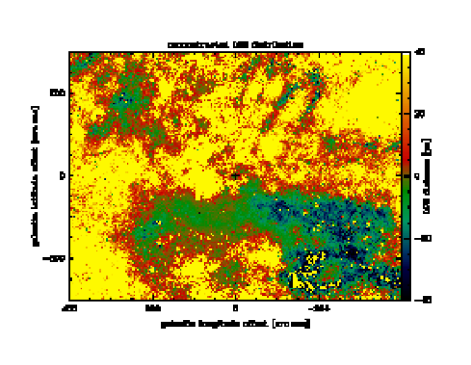
Figure 14: Map of the reconstructed LOS distances for the 2MASS K_S images. Upper panel: all blue point sources are subtracted. Lower panel: all point sources (blue and red) are subtracted.

In order to correlate the reconstructed LOS distribution with observed clouds we show in Fig. 15 the 1.2 mm observations of Zylka et al. (1998) together with the LOS distance distribution filtered with a median filter of 11 pixels.

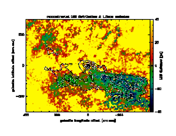
Figure 15: Contours: IRAM 30m 1.2 mm observations of Zylka et al. (1998). Colors: LOS distance distribution filtered with a median filter of 11 pixels.

As already shown by Philipp et al. (1999) the 50 km s^-1 and the 20 km s^-1 cloud complexes can be clearly seen at $200^{\prime\prime}>\Delta l>0^{\prime\prime}$ and $-50^{\prime\prime}>\Delta l>-300^{\prime\prime}$, respectively. The part of the 50 km s^-1 cloud near Sgr A^∗ is not seen in the 1.2 mm data, because of their observing mode (double beam mapping/chopping). The 50 km s^-1 cloud complex is located between 0 pc and 6 pc in front of Sgr A^∗ (cf. Fig. 12). We can identify a small gradient of the LOS distance parallel to the galactic longitude. From $\Delta l=150^{\prime\prime}$ to $\Delta l=50^{\prime\prime}$ the LOS distance increases from $-6$ pc to 0 pc. Then it drops again to $-4$ pc at $\Delta l\sim 20^{\prime\prime}$. This is best seen in the lower image of Fig. 14. The annex of the 50 km s^-1 cloud complex that is located at ($\Delta l\sim 200^{\prime\prime}$, $\Delta b\sim-150^{\prime\prime}$) and which has an elongation approximately perpendicular to the main 50 km s^-1 cloud complex is located nearer to the observer ($d\sim-10$ pc) than the main 50 km s^-1 cloud complex. We might tentatively see a gradient from large distances at small galactic latitudes to small distances at larger galactic latitudes, i.e. near the main 50 km s^-1 cloud complex. This cloud is also not seen in the 1.2 mm observations, because of the observing mode (double beam mapping/chopping). It clearly appears in the IRAM 30m CS(2-1) data (Güsten et al. in prep.; Fig. 16).

The 20 km s^-1 cloud complex shows a very patchy structure compared to the 50 km s^-1 cloud complex. It is not excluded that both consist of several distinct clouds. It has an overall LOS distance gradient from $\sim$0 pc at $\Delta l=-350^{\prime\prime}$ to $\sim-27$ pc at $\Delta l=-120^{\prime\prime}$ (cf. Fig. 12). The gradient becomes shallower for increasing $\Delta l$. For $-120^{\prime\prime}<\Delta l<-50^{\prime\prime}$ the gradient has the opposite sign, i.e. the 20 km s^-1 cloud complex approaches the Sgr A^∗. We observe a jump of the LOS distance at $\Delta l\sim-30^{\prime\prime}$ which might represent a discontinuity between the 20 and 50 km s^-1 cloud complexes, i.e. that both structures are not physically connected (F in Fig. 8).

Below the 20 km s^-1 cloud complex a large shell-like absorption feature can be seen ($\Delta l=-250^{\prime\prime}$, $\Delta b=-250^{\prime\prime}$) (A in Fig. 8). Since this structure does not appear in the 1.2 mm data nor in the CS(2-1) data, it must be a structure that is located distinnctly in front of the 20 km s^-1 cloud. In the maps of the reconstructed LOS distances it appears as a yellow region with blue borders. This means that this absorption feature is located at $z<-50$ pc. Since it is only this structure that shows negative absorption we are confident that the applied offset $a$=150 $\mu$Jy/arcsec² is acceptable. If $a$ was slightly larger, parts of the 20 km s^-1 cloud complex would have negative absorption feature, which would not be acceptable.

At positive galactic longitudes and latitudes an absorption feature shows up that is also located in front of Sgr A^∗ (C in Fig. 8). A comparison with the CS(2-1) data (Fig. 16) shows this cloud complex is really located in the Nuclear Bulge near Sgr A^∗.

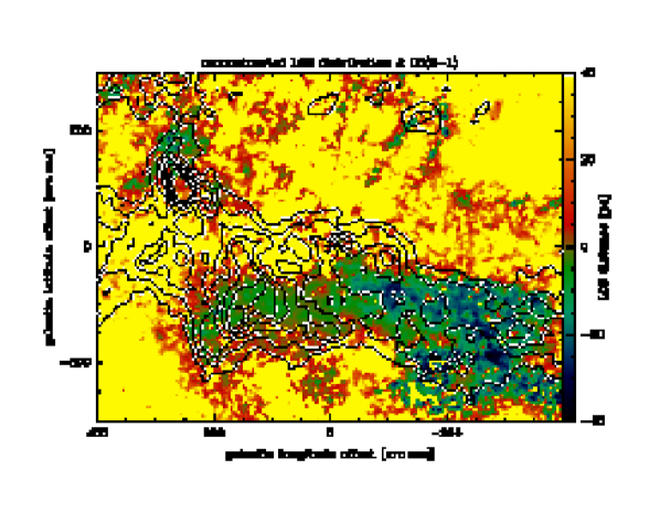
Figure 16: Contours: IRAM 30m CS(2-1) line observations (Güsten et al. in prep.) integrated over the whole velocity range. Colors: LOS distance distribution filtered with a median filter of 11 pixels.

At negative galactic longitudes and positive latitudes another shell-like structure can be seen (B in Fig. 8). If it was located at distances $<$50 pc to Sgr A^∗ it would be stretched within one rotation period, i.e. $<1$ Myr parallel to the galactic longitude, because of the strong shear motions in this region. Thus, we believe that it is most probably a foreground structure.

6 Discussion

The relative distances between the molecular cloud complexes and the relative gradients within them are robust results. The absolute distance of the 50 km s^-1 cloud complex is determined with a $\sim$20% error. This behaviour does not change significantly for different analytic profiles and different offsets $a$ and $z_{0}$ (Sect. 5.1). However, due to the nonlinearity of our reconstruction method (Fig. 11), the absolute distance of the 20 km s^-1 cloud complex strongly depends on the model profile. The LOS distance of the darkest subcloud of this complex varies between $-90$ pc using Eq. (3) and $a=-150$ $\mu$Jy/arcsec² and $-16$ pc using Eq. (2) and $a$=0. Since the profile of Eq. (3) overestimates the K_S band continuum emission (Fig. 10), we think that the these distances are too low. The main uncertainty comes from our ignorance regarding the sky subtraction, i.e. the absolute value of the K_S band intensity. We have to assume an absolute distance of cloud A (Fig. 8). The most plausible scenarios for us are (i) that the limit of integration is $z_{0}=-100$ pc, i.e. the extent of the Nuclear Bulge (Launhardt et al. 2002) and $a$=0 and (ii) that $a$=150 $\mu$Jy and $z_{0}=-50$ pc, which places cloud A at $z<-50$ pc. Both models lead to a very similar LOS distribution of the giant molecular cloud complexes (Fig. 12). However, it is not excluded that the LOS distances with respect to Sgr A^∗ of the 20 km s^-1 cloud complex might be underestimated by up to a factor of 2.

For a further discussion of the LOS distribution of the GMC complexes in the Galactic Center we show in Fig. 17 IRAM 30m CS(2-1) line observations (Güsten et al. in prep.). The integrated flux over channels $-140$ km s${}^{-1}<v<-31$ km s^-1 and 71 km s${}^{-1}<v<$115 km s^-1 corresponds to emission from the CND.

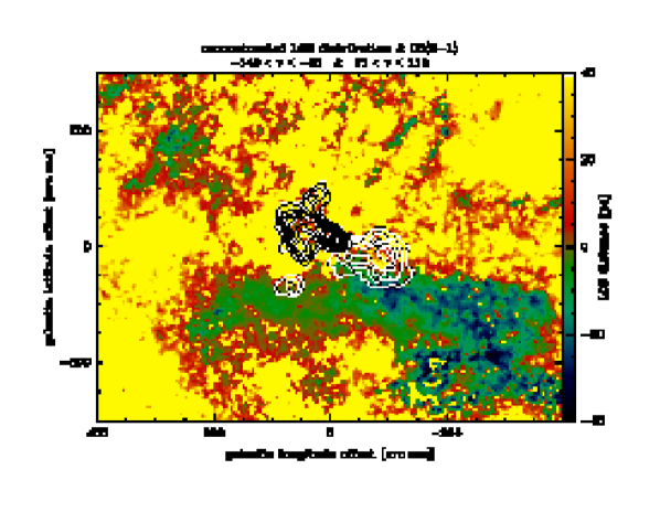
Figure 17: Contours: IRAM 30m CS(2-1) line observations (Güsten et al. in prep.). The integrated flux over channels $-140$ km s${}^{-1}<v<$-31 km s^-1 and 71 km s${}^{-1}<v<$115 km s^-1, i.e. the CND, are shown. Colors: LOS distance distribution filtered with a median filter of 11 pixels.

The bulk of the CND (except the western arc region) does not appear in the reconstructed LOS distance distribution. Since the CND does not cause absorption, its area filling factor must be very low. With an effective resolution of $\sim 3^{\prime\prime}$ (0.12 pc) this sets an upper limit for the cloud sizes of $\sim$0.06 pc. This is consistent with the findings of Jackson et al. (1993) who gave an upper limit of 0.1 pc.

It is a surprise that the Western Arc (Lacy et al. 1991) can be recognized in our LOS reconstruction (Fig. 15) at the right distance, i.e. $d\sim-(1{\rm-}2)$ pc (E in Fig. 8). This means that the clouds that are located in the Western Arc have a larger filling factor than those in the rest of the CND. We might speculate that this is linked to the mechanism that forms an inner edge proposed by Vollmer & Duschl (2001). They proposed a scenario where a clump of an external GMC is falling onto the CND. Clumps that have a low central density become stretched by the tidal shear. Thus, their area filling factor increases. This is one possibility to explain the K_S band absorption produced by the Western Arc.

7 Conclusions

We use 2MASS K_S images of the Galactic Center region to calculate the LOS distribution of the GMCs located within the inner 60 pc of the Galaxy. Using the H band image we distinguish two populations of point sources: a blue and a red population. The blue population represents a homogeneous screen of foreground stars and has to be subtracted from the K_S band image. We reconstructed the line-of-sight distance distribution assuming (i) an axis-symmetric stellar distribution and (ii) that the clouds are optically thick and have an area filling factor $\sim$1, i.e. that they block entirely the light from the stars located behind them. Due to the method of reconstruction, the LOS distances close to Sgr A^∗ ($-10\ {\rm pc}<d<10\ {\rm pc}$) have a small uncertainty, whereas it is not excluded that those of larger distances might be underestimated by up to a factor of 2. The relative distances are robust results. We conclude that

• all structures seen in the 1.2 mm observations (Zylka et al. 1998) and CS(2-1) observations (Güsten et al. in prep.) are present in absorption.

• the 50 km s^-1 cloud complex is located between 0 pc and $-5$ pc with an uncertainty of $\sim$20%, i.e. in front of Sgr A^∗. It has a small LOS distance gradient.

• the 20 km s^-1 cloud complex is located in front of the 50 km s^-1 cloud complex. The subclump of deepest absorption has a LOS distance between $-50$ pc and $-25$ pc.

• the 20 km s^-1 cloud complex shows a large LOS distance gradient with galactic longitude.

• the Western Arc of the Minispiral has a larger area filling factor than the rest of the CND.

• the bulk of the CND is not seen in absorption. This gives an upper limit of the cloud sizes within the CND of $\sim$0.06 pc.

- (1) Coil A.L. & Ho T.P.T. 1999, ApJ, 513, 752
- (2) Coil A.L. & Ho T.P.T. 2000, ApJ, 533, 245
- (3) Dent W.R.F., Matthews H.E., Wade R., & Duncan W.D. 1993, ApJ 410, 650
- (4) DePoy D.L., Gatley I., & McLean I.S. 1989, IAU-Symp. 136, 361
- (5) Eckart A. & Genzel R. 1996, Nature 383, 415
- (6) Ekers R.D., Goss W.M., Schwarz U.J., Downes D., & Rogstad D.H. 1975, A&A, 43, 159
- (7) Gatley I., Jones J.J., Hyland A.R. et al. 1986, MNRAS 222, 299
- (8) Güsten R., Genzel R., Wright M.C.H. et al. 1987, ApJ 318, 124
- (9) Jackson J.M., Geis N., Genzel R. et al. 1993, ApJ 402, 173
- (10) Lacy J.H., Achtermann J.M., & Serabyn E. 1991, ApJ 380, L71
- (11) Launhardt R., Zylka R., Mezger P.G. 2002, A&A, 384, 112
- (12) Lo K.Y. & Claussen M.J. 1983, Nature 306, 647
- (13) Marr J.M., Wright M.C.H., & Backer D.C. 1993, ApJ 411, 667
- (14) Mathis J., Mezger P.G., & Panagia N. 1983, A&A, 128, 212
- (15) Mezger P.G., Zylka R., Salter C.J. et al. 1989, A&A 209, 337
- (16) Mezger P.G., Zylka R., Philipp S., & Launhardt R. 1999, A&A, 348, 457
- (17) Philipp S., Zylka R., Mezger P.G. et al. 1999, A&A, 348, 768
- (18) Serabyn E., Güsten R., Walmsley C.M. et al. 1986, A&A 169, 85
- (19) Sutton E.C., Danchi W.C., Jaminet P.A., & Masson C.R. 1990, ApJ 348, 503
- (20) Vollmer B. & Duschl W.J. 2001, A&A, 377, 1016
- (21) Wright M.C.H., Coil A.L., McGary R.S., Ho P.T.P., & Harris A.I. 2001, ApJ, 551, 254
- (22) Yusef-Zadeh F., Roberts D.A., Goss W.M. et al. 1996, ApJL, 466, L27
- (23) Zylka R., Mezger P.G., & Wink J.E. 1990, A&A, 234, 133
- (24) Zylka R., Philipp S., Duschl W.J., et al. 1998, in: The central regions of the Galaxy and galaxies, Proceedings of the 184th symposium of the International Astronomical Union, held in Kyoto, Japan, August 18-22, 1997. Edited by Yoshiaki Sofue. Publisher: Dordrecht: Kluwer, p.291