Angular Spectra of Polarized Galactic Foregrounds

Abstract

It is believed that magnetic field lines are twisted and bend by turbulent motions in the Galaxy. Therefore, both Galactic synchrotron emission and thermal emission from dust reflects statistics of Galactic turbulence. Our simple model of Galactic turbulence, motivated by results of our simulations, predicts that Galactic disk and halo exhibit different angular power spectra. We show that observed angular spectra of synchrotron emission are compatible with our model. We also show that our model is compatible with the angular spectra of star-light polarization for the Galactic disk. Finally, we discuss how one can estimate polarized microwave emission from dust in the Galactic halo using star-light polarimetry.

1 Introduction

Exciting possibilities of measuring spectrum of polarized cosmic microwave background (CMB) fluctuations renewed the interest to the polarized fluctuations of Galactic origin. Synchrotron and dust are known to be the most important sources of polarized foreground radiation. Measurements of angular power spectra of such foregrounds are of great interest. So far, a large number of observations are available for angular power spectra of synchrotron emission and synchrotron polarization for Galactic disk and halo (see papers in de Oliveira-Costa & Tegmark 1999; see also references listed in §2 and papers in this volume). Those measurements revealed a range of power-laws, the origin of which has been addressed by Chepurnov (2002) and Cho & Lazarian (2002a; henceforth CL02). The latter also addressed the origin of the observed angular spectrum of starlight polarization (Fosalba et al. 2002; henceforth FLPT).

Interstellar medium is turbulent and Kolmogorov-type spectra were reported on the scales from several AU to several kpc (see Armstrong, Rickett, & Spangler 1995; Lazarian & Pogosyan 2000; Stanimirovic & Lazarian 2001; Lazarian & Esquivel 2003). Therefore it is natural to think of the turbulence as the origin of the fluctuations of the diffuse foreground radiation. Interstellar medium is magnetized with magnetic field making turbulence anisotropic. It may be argued that although the spectrum of MHD turbulence exhibits scale-dependent anisotropy if studied in the system of reference defined by the local magnetic field (Goldreich & Sridhar 1995; Lithwick & Goldreich 2001; Cho & Lazarian 2002b,2003ab), in the observer’s system of reference the spectrum will show only moderate scale-independent anisotropy. Thus from the observer’s perspective Kolmogorov’s description of interstellar turbulence statistics is acceptable in spite of the fact that magnetic field is dynamically important and even dominant (see discussion in Lazarian & Pogosyan 2000; Cho, Lazarian, & Vishniac 2003).

In this paper, we claim that MHD turbulence can explain observed angular spectra of Galactic synchrotron emission and starlight polarization. For this purpose, we use an analytical insight obtained in Lazarian (1992, 1995ab) and numerical results obtained in CL02.. We also discuss how we can estimate polarized microwave dust emission using star-light polarimetry. This problem is of great importance in view of recent interest to the foregrounds to the CMB polarization (see also review by Lazarian in this volume).

2 Galactic synchrotron emission

2.1 Summary of observations

It is customary for CMB studies to expand the foreground intensity over spherical harmonics $Y_{lm}$, $I(\theta,\phi)=\sum_{l,m}a_{lm}Y_{lm}(\theta,\phi)$, and write the spectrum in terms of $C_{l}\equiv\sum_{m=-l}^{m=l}|a_{lm}|^{2}/(2l+1)$. The measurements indicate that angular power spectrum ($C_{l}$) of the Galactic emission follows power law ($C_{l}\propto l^{-\alpha}$) (see FLPT and references in §3). The multipole moment $l$ is related to the angular scale $\theta$ on the sky as $l\sim\pi/\theta^{radian}$ (or $l\sim 180^{\circ}/\theta^{\circ}$). When the angular size of the observed sky patch ($\Delta\theta\times\Delta\theta$ in radian) is small, $C_{l}$ is approximately the ‘energy’ spectrum of fluctuations (Bond & Efstathiou 1987; Hobson & Majueijo 1996; Seljak 1997). It is this power spectrum expressed in terms of wavenumber $k~{}(\sim l\,\Delta\theta/\pi)$ that is usually dealt with in studies of astrophysical turbulence (e.g. Stanimirovic & Lazarian 2001).

Recent statistical studies of total synchrotron intensity include Haslam all-sky map at 408 MHz (Haslam et al. 1982) that shows that the angular power index $\alpha$ ($C_{l}\propto l^{-\alpha}$) is in the range between 2.5 and 3 (Tegmark & Efstathiou 1996; Bouchet, Gispert, & Puget 1996). Parkes southern Galactic plane survey (Duncan et al. 1997) at 2.4 GHz suggests shallower slope: Giardino et al. (2002) obtained $\alpha\sim 2.05$ after point source removal and Baccigalupi et al. (2001) obtained $\alpha\sim 0.8$ to $2$. On the other hand, Tucci et al. (2000) obtained $\alpha\sim 1.4$ to $1.8$ and Bruscoli et al. (2002) obtained $\alpha\sim 0.4$ to $2.2$ for the Galactic disk. Using Rhodes/HartRAO data at 2326 MHz (Jonas, Baart, & Nicolson 1998), Giardino et al. (2001a) obtained $\alpha\sim 2.43$ for all-sky data and $\alpha\sim 2.92$ for high Galactic latitude regions with $|b|>20^{\circ}$. Giardino et al. (2001b) obtained $\alpha\sim 3.15$ for high Galactic latitude regions with $|b|>20^{\circ}$ from Reich & Reich (1986) survey at 1420 MHz. The rough tendency that follow from these data is that $\alpha$ which is close to $2$ for the Galactic plane gets steeper (to $\sim 3$) for higher latitudes (Fig. 1a).

Can we explain this tendency? In the next section, we construct a simple model that can explain the rough tendency of observed angular spectra.

2.2 Basic idea of our simple model

2.2.1 $C_{l}$ for small angle limit

In this section we show that, when the angle between the lines of sight is small (i.e. $\theta<L/d_{max}$), the angular spectrum $C_{l}$ has the same slope as the 3-dimensional energy spectrum of turbulence. Here $L$ is the typical size of the largest energy containing eddies, which is sometime called as outer scale of turbulence or energy injection scale, and $d_{max}$ is the distance to the farthest eddies (see Fig. 1b).

To illustrate the problem consider the observations with lines of sight being parallel. The observed intensity is the intensity summed along the line of sight, $r_{z}$:

$${I}_{2D}(r_{x},r_{y}) \equiv \int d{r_{z}}~{}i_{3D}({\bf r})$$ (1)

$$= \int d{r_{z}}\ \int dk_{x}dk_{y}dk_{z}\ \hat{i}_{3D}({\bf k})\ e^{i{\bf k}\cdot{\bf r}}.$$ (2)

Rearranging the order of summation and using $\int d{r_{z}}\ e^{ik_{z}r_{z}}=\delta(k_{z})$, we get

$${I}_{2D}(r_{x},r_{y})=\int d{k_{x}}dk_{y}~{}\hat{i}_{3D}(k_{x},k_{y},0)~{}e^{ik_{x}r_{x}+ik_{y}r_{y}},$$ (3)

which means Fourier transform of ${I}_{2D}(r_{x},r_{y})$ is $\hat{i}_{3D}(k_{x},k_{y},0)$. As it was mentioned earlier for small patches of sky $C_{l}\sim|\hat{i}_{3D}(k_{x},k_{y},0)|^{2}$ with $l\sim k(\pi/\Delta\theta)$ and $k=(k_{x}^{2}+k_{y}^{2})^{1/2}$.

The analysis of the geometry of crossing lines of sight is more involved, but for power-law statistics it follows from Lazarian & Shutenkov (1990) that if $|\hat{i}_{3D}|^{2}\propto k^{-m}$, then the ‘energy’ spectrum of ${I}_{2D}(r_{x},r_{y})$ is also $k^{-m}$. Therefore, we have

$$C_{l}\propto|\hat{i}_{3D}(k_{x},k_{y},0)|^{2}\propto l^{-m}.$$ (4)

in the small $\theta$ limit. For Kolmogorov turbulence ($|\hat{i}_{3D}|^{2}\propto k^{-11/3}$), we expect

$$C_{l}\propto l^{-11/3},\mbox{~{}~{}~{}if $\theta<L/d_{max}$.}$$ (5)

Note that $l\sim\pi/\theta$.

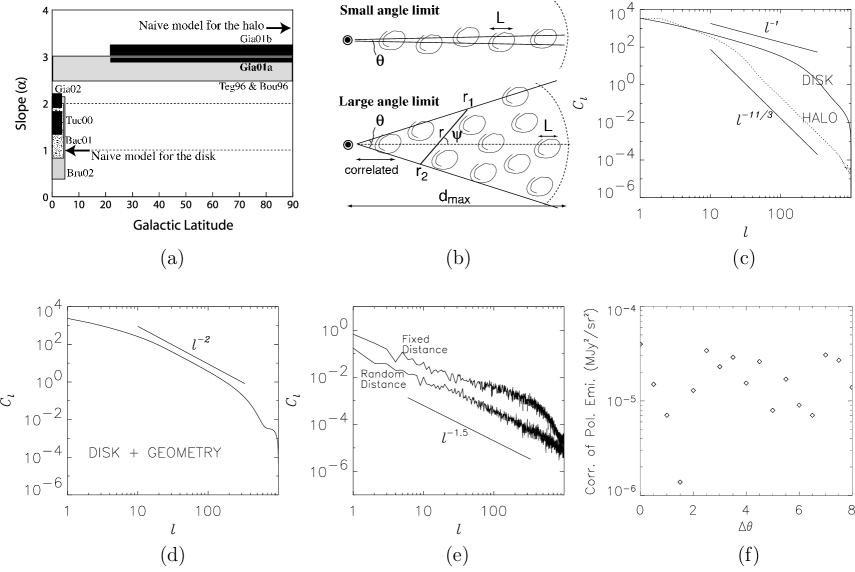
Figure 1: (a) Comparison with observations. Widths of rectangles correspond to the Galactic latitude of the observed patches. Heights of rectangles denote either error bars or scatter of the slopes. (Gia02=Giardino et al. 2002; Bru02=Bruscoli et al. 2002; etc.). (b) Upper plot: Small $\theta$ limit ($\theta<L/d_{max}$). The fluctuations along the entire length of the lines of sight are correlated. Lower plot: Large $\theta$ limit ($\theta>L/d_{max}$). Only points close to the observer are correlated. (c) Spectra for the disk ($d_{max}$ = 10 kpc; turbulence size $L$ = 100 pc) and for the halo ($d_{max}$ = 1 kpc; turbulence size $L$ = 100 pc). (d) Angular spectrum for the Galactic disk. We considered the geometry of the Galactic disk. (e) Angular spectra of degree of polarization. Fixed Distance means all stars are at the same distance of 10 kpc. Random Distance means random sampling of stars according to equation (3). Zero points of $C(\theta)$ and $C_{l}$’s are arbitrary. (f) Angular correlation function for polarized intensity at 1mm. From eq. (16). Figure (a)-(e) are from CL02.

2.2.2 $C_{l}$ for large angle limit

Following Lazarian & Shutenkov (1990), we can show that the angular correlation function for $\theta>L/d_{max}$ is given by

$$K(\theta) = \int\int dr_{1}dr_{2}~{}{\cal K}(|{\bf r}_{1}-{\bf r}_{2}|),$$ (6)

$$= \frac{1}{\sin{\theta}}\int_{0}^{\infty}dr~{}r{\cal K}(r)\int_{0}^{\pi/2}d\psi\sim\frac{const}{\theta},$$

where we change variables from $(r_{1},r_{2})$ to $(r,\psi)$, which is clear from Fig. 1b. We accounted for the fact that the Jacobian of the transformation is $r/\sin{\theta}$. We can understand $1/\theta$ behavior qualitatively from Fig. 1a. When the angle is large, the points along of the lines of sight near the observer are still correlated. These points extend from the observer over the distance $\propto 1/\sin{(\theta/2)}$.

In the limit of $\theta\ll 1$ we get the angular power spectrum $C_{l}$ using Fourier transform:

$$C_{l} \sim \int\int K(\theta)e^{-i{\bf l}\cdot{\bf\theta}}d\theta_{x}d\theta_{y}$$ (7)

$$\sim \int d\theta~{}\theta J_{0}(l\theta)K(\theta)\propto l^{-1},$$

where $\theta=(\theta_{x}^{2}+\theta_{y}^{2})^{1/2}$, $J_{0}$ is the Bessel function, and we use $K(\theta)\propto\theta^{-1}$.

In summary, for Kolmogorov turbulence, we expect from equations (5) and (7) that

$$C_{l}\propto\left\{\begin{array}[]{ll}l^{-11/3}&\mbox{if $l>l_{cr}$}\\ l^{-1}&\mbox{if $l<l_{cr}$.}\end{array}\right.$$ (8)

which means that the power index $\alpha$ of $C_{l}$ is $-1\leq\alpha\leq-11/3$. The critical multipole moment $l_{cr}~{}(\sim 3\,d_{max}/L)$ depends on the size of the large turbulent eddies and on the direction of the observation. If in the naive model we assume that turbulence is homogeneous along the lines of sight and that $L\sim 100$ pc, corresponding to a typical size of the supernova remnant, we get $l_{cr}\sim 300$ for the Galactic disk with $d_{max}\sim 10$ kpc. For the synchrotron halo, $d_{max}\sim 1$ kpc (see Smoot 1999) and we get $l_{cr}\sim 30$.

2.3 Numerical results

Can this model really explain observed behavior of synchrotron angular spectrum? To address the problem, we perform simple numerical calculations for the Galactic disk and halo. We obtain $C_{l}$ using the relation

$$K(\cos\theta)=\frac{1}{4\pi}\sum_{l}(2l+1)C_{l}P_{l}(\cos{\theta}),$$ (9)

$$C_{l}=\frac{1}{2}\int P_{l}(\cos{\theta})K(\cos\theta)\ d(\cos\theta).$$ (10)

We use Gauss-Legendre quadrature integration (see Szapudi et al. 2001 for its application to CMB) to obtain $C_{l}$. We numerically calculate the angular correlation function from

$$K(\cos{\theta})=\int dr_{1}\int dr_{2}~{}{\cal K}(|{\bf r}_{1}-{\bf r}_{2}|),$$ (11)

where $|{\bf r}_{1}-{\bf r}_{2}|=r_{1}^{2}+r_{2}^{2}-2r_{1}r_{2}\cos{\theta}$ and assume that the spatial correlation function ${\cal K}(r)$ follow Kolmogorov statistics:

$${\cal K}(r)\propto\left\{\begin{array}[]{ll}{\cal K}_{0}-r^{2/3}&\mbox{if $r<L$}\\ 0&\mbox{if $r>L$,}\end{array}\right.$$ (12)

where ${\cal K}_{0}\sim L^{2/3}$ is a constant. Fig. 1c illustrates the agreement of our calculations with the theoretical expectations within the naive model of the disk and the halo from the previous section.

2.4 A more realistic model for Galactic disk

The naive model discussed in the previous section predicts $l^{-1}$ spectrum for the Galactic disk for $l<300$ (see Fig. 1c and the discussion below eq. (8)). However, as we discussed earlier, observations show angular spectra close to $l^{-2}$. In other words $2\leq\alpha\leq 3$ which differs from naive expectations given by equation (8).

To make the spectrum closer to observations we need to consider more realistic models. First, synchrotron emission is stronger in spiral arms, and therefore we have more synchrotron emission coming from the nearby regions. Second, if synchrotron disk component is sufficiently thin, then lines of sight are not equivalent and effectively nearby disk component contributes more. Indeed, when we observe regions with low Galactic latitude, the effective line of sight varies with Galactic latitude.

Suppose we observe a region with $b=10^{\circ}$. Then emission from $d=10$ kpc is substantially weaker than that from $d=100$ pc, because the region with $d=10$ kpc is $d\sin{10^{\circ}}\sim 1.7$ kpc above the Galactic plane and, therefore, has weak emission. To incorporate the effect of finite thickness ($\sim 100$ pc) of the disk, we use the weighting function $w(r)=100pc/\mbox{max}(100pc,r\sin{10^{\circ}})$, which gives more weight to closer distances. The resulting angular power spectrum (Fig. 1d) shows a slope similar to -2.

For the halo, the simple model predicts that $C_{l}\propto l^{-11/3}$ for $l>30$, but observations provide somewhat less steep spectra. Is this discrepancy very significant? The spectrum of magnetic field is expected to be shallower than $k^{-11/3}$ in the vicinity of the energy injection scale and at the vicinity of the magnetic equipartition scale. The observed spectrum also gets shallower if $d_{max}$ gets larger. For instance Beuermann, Kanbach, & Berkhuijsen (1985) reported the existence of thick radio halo that extends to more than $\sim 3~{}kpc$ near the Sun. Finally, filamentary structures and point sources can make the spectrum shallower as well. Further research should establish the true reason for the discrepancy.

3 MHD turbulence and Galactic Starlight Polarization

Let us move to a different topic - starlight polarization. In this section, we will illustrate that MHD turbulence can explain the observed angular spectrum of starlight polarization.

Polarized radiation from dust is an important component of Galactic foreground that strongly interferes with intended CMB polarization measurements (see Lazarian & Prunet 2001). FLPT attempted to predict the spectrum of the polarized foreground from dust and obtained $C_{l}\sim l^{-1.5}$ for starlight polarization degree. They used polarization data from $\sim$5500 stars. The sample is strongly biased toward nearby stars ($d<2$ kpc) within the Galactic plane. This spectrum is different from those discussed in the previous sections. To relate this spectrum to the underlying turbulence we should account for the following facts: a) the observations are done for the disk component of the Galaxy, b) the sampled stars are at different distances from the observer with most of the stars close-by.

To deal with this problem we use numerical simulations again. We first generate a three (i.e. x,y, and z) components of magnetic field on a two-dimensional plane ($4096\times 4096$ grid points representing $10$ kpc $\times$ $10$ kpc), using the following Kolmogorov three-dimensional spectrum: $E_{3D}(k)\propto k^{-11/3}$ if $k>k_{0}$, where $k_{0}\sim 1/100$pc. Our results show that the way how we continuously extend the spectrum for $k<k_{0}$ does not change our results.

To simulate the actual distribution of stars within the sample used in FLPT, we scatter our emission sources using the following probability distribution function: $P(r)\propto e^{-r/1.5kpc}.$ The starlight polarization is due to the difference in absorption cross section of non-spherical grains aligned with their longer axes perpendicular to magnetic field (see a review by Lazarian 2003). In numerical calculations we approximate the actual turbulent magnetic field by a superposition of the slabs with locally uniform magnetic field in each slap and assume that the difference in grain absorption parallel and perpendicular to magnetic field results in the 10% difference in the optical depths $\tau_{\|}$ and $\tau_{\bot}$ for a slab. We calculate evolution of Stokes parameters of the starlight within the slab and use the standard transforms of Stokes parameters from one slab to another (Dolginov, Gnedin, & Silantev 1996; see similar expressions in Martin 1972).

We show the result in Fig. 1e. For comparison, we also calculate the degree of polarization assuming all stars are at the same distance of $\sim 10$ kpc. The result shows that, for a mixture of nearby and faraway stars, the slope steepens and gets very close to the observed one, i.e. $-1.5$.

4 Estimation of Polarized Emission from Dust

One of the possible ways to estimate the polarized radiation from dust at the microwave range is to measure star-light polarization and use the standard formulae relating polarization at different wavelength. The technique can be traced back to FLPT. In this section, we estimate polarized diffuse emission by dust in the high Galactic latitude halo. For our practical data handling, see Hildebrand et al. (1999). We use the data of optical depth (in fact, $E(B-V)$) and the degree of polarization by absorption $P_{abs,optical}$ for stars in the halo (provided by Terry Jones).

When the optical depth is small, we have the following relation (see, for example, Hildebrand et al. 2000):

$$P_{em,optical}\approx-P_{abs,optical}/\tau,$$ (13)

where $P_{em,optical}$ is the degree of polarization by emission and $\tau$ is the optical depth (at optical wavelengths). We obtain polarization by emission at 1mm ($P_{em,mm}$) using the relation

$$P_{em,mm}=P_{em,optical}\left[\frac{C_{max}-C_{min}}{C_{max}-C_{min}}\right]_{mm}/\left[\frac{C_{max}-C_{min}}{C_{max}-C_{min}}\right]_{optical},$$ (14)

where $C$’s are cross sections that depend on the geometrical shape (see, for example, the discussion in Hildebrand et al. 1999; see also Draine & Lee 1984) and dielectric function $\epsilon$ (see Draine 1985) of grains. We assume grains are 2:1 oblate spheroids.

We can obtain the emission at 1mm ($I_{mm}$) from that at 100 $\mu m$ ($I_{100\mu m}$):

$$I_{mm}=I_{100\mu m}(1mm/100\mu m)^{-\beta},$$ (15)

where we use $\beta\sim 1.7$. For now, we assume that $I_{100\mu m}\approx 0.85$ MJy/sr (Boulanger & Perault 1988; see also Draine & Lazarian 1998). From this, we obtain $I_{mm}\approx 0.017$ MJy/sr. In the future, we can use an actual $100\mu m$ map to get $I_{mm}$.

From $P_{em,mm}$ and $I_{mm}$, we can easily obtain the polarized intensity at 1mm ($I_{pol,mm}$):

$$I_{pol,mm}=P_{em,mm}I_{mm}.$$ (16)

Fig. 1f, obtained this way, shows $I_{pol,mm}$.

Last step will be the estimation of the angular spectrum $C_{l}$. From CL02 (see also §2.2), we obtain

$$C_{l}\approx\left\{\begin{array}[]{ll}Al^{-1}&\mbox{ if $l<30$ }\\ 30^{8/3}Al^{-11/3}&\mbox{ if $l>30$, }\end{array}\right.$$ (17)

where A is a constant that is determined by $\sum l(l+1)C_{l}\approx 10^{-5},$ where $10^{-5}$ is the rms fluctuation (see y-axis of Fig. 1f). Calculation yields $A=10^{-5}/30^{2}$. Therefore,

$$C_{l}\approx\left\{\begin{array}[]{ll}10^{-7}l^{-1}~{}~{}(MJy^{2}/sr^{2})&\mbox{ if $l<30$ }\\ 10^{-4}l^{-11/3}~{}~{}(MJy^{2}/sr^{2})&\mbox{ if $l>30$. }\end{array}\right.$$ (18)

When we prefer $(\mu K)$ to $(MJy/sr)$, we can use the conversion factor $c_{*}\approx(1/x^{2})(10^{4}\mu K/(MJy/sr))$, where $x\approx\nu/56.8$ GHz (Tegmark et al. 2000). For 1mm, $x\approx 5$ and $c_{*}\approx 400$. $C_{l}c_{*}^{2}$ gives

$$C_{l}\approx\left\{\begin{array}[]{ll}10^{-2}l^{-1}~{}~{}(\mu K^{2})&\mbox{ if $l<30$ }\\ 10l^{-11/3}~{}~{}(\mu K^{2})&\mbox{ if $l>30$. }\end{array}\right.$$ (19)

The particular normalization coefficients and the spectral index may vary from one region to another (see FLPT; CL02).

We can summarize the procedure as follows:

$$\left.\begin{array}[]{crl}P_{abs,optical}&\rightarrow P_{em,optical}&\rightarrow P_{em,mm}\\ &I_{100\mu m}&\rightarrow I_{mm}\end{array}\right\}\rightarrow C_{l}\mbox{~{}(at 1 mm)}$$ (20)

5 Summary

In this paper we have addressed the origin of spatial fluctuations of Galactic diffuse emission. We have shown that MHD turbulence with Kolmogorov spectrum can qualitatively explain the observed properties of synchrotron emission and starlight polarization. The variety of measured spatial spectra of synchrotron emission can be accounted for by the inhomogeneous distribution of emissivity along the line of sight arising from the structure of the Galactic disk and halo. Similarly, MHD turbulence plus inhomogeneous distribution of stars can explain the reported scaling of starlight polarization statistics. Although these complications do not allow to predict the exact slope of the measured fluctuations, our interpretation allows a valuable qualitative insight on what sort of change is to be expected.

We have shown that one can estimate polarized diffuse micro-wave emission by dust using star-light. Our preliminary result shows that $\delta T\sim[l(l+1)C_{l}]^{1/2}\sim O(1)\mu K$ for high Galactic latitude regions.

Evidently more systematic studies are required. Those studies will not only give insight into how to separate CMB from foregrounds, but also would provide valuable information on the structure of interstellar medium and the sources/energy injection scales of interstellar turbulence. (See also review by Lazarian, this volume.)

Acknowledgments We acknowledge the support of NSF Grant AST-0125544.

References

- [1] Armstrong, J., Rickett, B., & Spangler, S. 1995, ApJ, 443, 209
- [2] Baccigalupi, C., Burigana, C., Perrotta, F., De Zotti, G., La Porta, L., Maino, D., Maris, M., & Paladini, R. 2001 A&A, 372, 8
- [3] Beuermann, K., Kanbach, G., & Berkhuijsen, E. 1985, A&A, 153, 17
- [4] Bond, J.R. & Efstathiou, G. 1987, MNRAS, 226, 655
- [5] Bouchet, F.R., Gispert, R., & Puget, J.L. 1996, in Unveiling the Cosmic Infrared Background, AIP Conf. Proc. 348, ed. E. Dwek (Baltimore: AIP), 225
- [6] Boulanger, F. & Perault, M. 1988, ApJ, 330, 964
- [7] Bruscoli, M., Tucci, M., Natale, V., Carretti, E., Fabbri, R., Sbarra, C., & Cortiglioni, S. 2002, NewA, 7, 171
- [8] Chepurnov, A. V. 2002, astro-ph/0206407 (Astron.Astrophys.Trans. 17 (1999) 281-300)
- [9] Cho,J. & Lazarian, A. 2002a, ApJL, 575, L63 (CL02)
- [10] Cho, J. & Lazarian, A. 2002b, Phy. Rev. Lett., 88, 245001
- [11] Cho, J., Lazarian, A., & Vishniac, E. T. 2003, in Turbulence and Magnetic Fields in Astrophysics, eds. E. Falgarone & T. Passot (Springer LNP), p56 (astro-ph/0205286)
- [12] de Oliveira-Costa, A. & Tegmark, M. 1999, Microwave Foregrounds, ASP Conf. Ser. 181, (San Francisco: ASP)
- [13] Dolginov, A. Z., Gnedin, Iu. N., & Silantev, N. A. 1996, Propagation and Polarization of Radiation in Cosmic Media, (Gordon & Breech)
- [14] Draine, B. 1985, ApJS, 57, 587
- [15] Draine, B. & Lazarian, A. 1998, ApJL, 494, L19
- [16] Draine, B. & Lee, H. 1984, ApJ, 285, 89
- [17] Duncan, A. R., Haynes, R. F., Jones, K. L., & Stewart, R. T. 1997, MNRAS, 291, 279
- [18] Fosalba, P., Lazarian, A., Prunet, S., & Tauber, J.A. 2002 ApJ, 564, 762 (FLPT)
- [19] Giardino, G., Banday, A.J., Fosalba, P., Górski, K.M., Jonas, J.L., O’Mullane, W., & Tauber, J. 2001a, A&A, 371, 708
- [20] Giardino, G., Banday, A. J., Bennett, K., Fosalba, P., Górski, K. M., O’Mullane, W., Tauber, J., & Vuerli, C. 2001b, in Mining the Sky, ed. A. J. Banday et al. (Springer-Verlag), 458 (astro-ph/0011084)
- [21] Giardino, G., Banday, A.J., Górski, K.M., Bennett, K., Jonas, J.L., & Tauber, J. 2002, A&A, 387, 82
- [22] Goldreich, P. & Sridhar, H. 1995, ApJ, 438, 763
- [23] Haslam, C.G.T., Stoffel, H., Salter, C.J., & Wilson, W.E. 1982, A&AS, 47, 1
- [24] Hildebrand, R. et al. 2000, PASP, 112, 1215
- [25] Hildebrand, R. et al. 1999, ApJ, 516, 834
- [26] Hobson, M.P. & Magueijo, J. 1996, MNRAS, 283, 1133
- [27] Jonas, J. L., Baart, E. E., & Nicolson, G. D. 1998, MNRAS, 297, 977
- [28] Lazarian, A. 1992, Astron. & Astrophys. Trans., 3, 33
- [29] Lazarian, A. 1995a, Ph. D. Thesis (Univ. of Cambridge, UK)
- [30] Lazarian, A. 1995b, A&A, 293, 507
- [31] Lazarian, A. 2003, J. of Quantitative Spectroscopy & Rad. Transf., 79-80, 881
- [32] Lazarian, A. & Esquivel, A. 2003, ApJL, in press (astro-ph/0304007)
- [33] Lazarian, A. & Pogosyan, D. 2000, ApJ, 537, 720
- [34] Lazarian, A. & Prunet, S. 2001, in Astrophysical Polarized Backgrounds, AIP Conf. Proc. 609, ed. S. Cecchini et al. (Melville: AIP), 32
- [35] Lazarian, A. & Shutenkov, V. P. 1990, PAZh, 16, 690 (translated Sov. Astron. Lett., 16, 297)
- [36] Lithwick, Y. & Goldreich, P. 2001, ApJ, 562, 279
- [37] Martin, P. G. 1972, MNRAS, 159, 179
- [38] Reich, P. & Reich, W. 1986, A&AS, 63, 205
- [39] Seljak, U. 1997, ApJ, 482, 6
- [40] Smoot, G. F. 1999, in Microwave Foregrounds, ASP Conf. Ser. 181, ed. A. de Oliveira-Costa & M. Tegmark (San Francisco: ASP), 61
- [41] Stanimirovic, S., & Lazarian, A. 2001, ApJ, 551, L53
- [42] Szapudi, I., Prunet, S., Pogosyan, D., Szalay, A. S., & Bond, J. R. 2001, ApJ, 548, L115
- [43] Tegmark, M. & Efstathiou, G. 1996, MNRAS, 281, 1297
- [44] Tegmark, M., Eisenstein, D. J., Hu, W., de Oliveira-Costa, A. 2000, ApJ, 530, 133
- [45] Tucci, M., Carretti, E., Cecchini, S., Fabbri, R., Orsini, M., & Pierpaoli, E. 2000, NewA, 5, 181