Two Dimensional Adiabatic Flows onto a Black Hole: I. Fluid Accretion

Abstract

When gas accretes onto a black hole, at a rate either much less than or much greater than the Eddington rate, it is likely to do so in an “adiabatic” or radiatively inefficient manner. Under fluid (as opposed to MHD) conditions, the disk should become convective and evolve toward a state of marginal instability. The resulting disk structure is “gyrentropic,” with convection proceeding along common surfaces of constant angular momentum, Bernoulli function and entropy, called “gyrentropes.” We present a family of two-dimensional, self-similar models which describes the time-averaged disk structure. We then suppose that there is a self-similar, Newtonian torque and that the Prandtl number is large. This torque drives inflow and meridional circulation and the resulting flow is computed. Convective transport will become ineffectual near the disk surface. It is conjectured that this will lead to a large increase of entropy across a “thermal front” which we identify as the effective disk surface and the base of an outflow. The conservation of mass, momentum and energy across this thermal front permits a matching of the disk models to self-similar outflow solutions. We then demonstrate that self-similar disk solutions can be matched smoothly onto relativistic flows at small radius and thin disks at large radius. This model of adiabatic accretion is contrasted with some alternative models that have been discussed recently. The disk models developed in this paper should be useful for interpreting numerical, fluid dynamical simulations. Related principles to those described here may govern the behaviour of astrophysically relevant, magnetohydrodynamic disk models.

1 Introduction

Recent X-ray observations of putative black holes in the nuclei of nearby elliptical galaxies show that they are extremely underluminous, some eight and four orders of magnitude below the Eddington and Bondi luminosities, respectively (e.g.,  Di Matteo et al., 2000; Baganoff et al., 2001; Mushotzky et al., 2000). These observations have stimulated a fresh look at the nature of the accretion process. It appears that when the hole is “underfed,” specifically when the mass accretion rate is well below the fiducial Eddington rate, $\dot{m}\equiv\dot{M}/\dot{M}_{E}\ll 1$, where $\dot{M}_{E}=4\pi GM/c\kappa$ (with $M$ denoting the black hole mass and $\kappa$, the relevant opacity), the radiative efficiency may be quite small, up to six orders of magnitude smaller than the traditional value $\sim 0.1\ c^{2}\sim 10^{20}$ erg g^-1.

One rationalisation of this observation (e.g.,  Quataert & Narayan, 1999, and references therein), is that the gas accretes quite rapidly under the action of viscous stress but the dissipated energy is taken up almost exclusively by the ions, which do not radiate directly and which cannot heat the electrons efficiently. In a large number of recent publications, it has been supposed that electrons are heated minimally in this manner and that there is a conservative inflow in which hot ions advect essentially all of their binding energy across the black hole event horizon.

However, these “Advection-Dominated Accretion Flow” (ADAF) solutions have a serious and fundamental shortcoming — the accreting gas is generically unbound and can escape to infinity. The reason why this happens is that the gas is likely to be supplied with sufficient angular momentum to orbit the hole and its inflow is controlled by the rate at which angular momentum is transported outward. This angular momentum transport, describable as a locally-acting torque, is necessarily associated with a transport of energy. If we attempt to conserve mass, angular momentum and energy in the flow, we find that the Bernoulli function — the energy that the gas would have if it were allowed to expand adiabatically to infinity — is twice the local kinetic energy (Blandford & Begelman, 1999, henceforth BB99). In conventional accretion disks, this energy is radiated away and the gas remains bound. However, when cooling is unimportant on the inflow time — we call this case “adiabatic” by analogy with the terminology for supernova remnants — something else must happen to the energy.

In an alternative description of adiabatic accretion, BB99 proposed that the inflow is non-conservative and that the radial energy transport drives an outflow that carries away mass, angular momentum and energy, allowing the disk to remain bound to the hole. (This was not a new proposal. Shakura & Sunyaev (1973) were aware of this possibility and it has been discussed in many subsequent studies.) In these “ADiabatic Inflow-Outflow Solutions” (ADIOS), the final accretion rate into the hole may be only a tiny fraction (in extreme cases $<10^{-5}$) of the mass supply at large radius (although this is not required). This leads to a much smaller luminosity than would be observed from a conservative flow. This is important from an observational perspective, because different assumptions about the extent and nature of the outflow affect the derived densities, temperatures, etc., of the emitting regions, and can lead to very different conclusions based on phenomenological fits to multi-band data. In particular, most ADAF models posit essentially thermal emission, whereas ADIOS models are supposed to involve nonthermal emission by relativistic electrons as may be accelerated in the trans-sonic, shearing, magnetized flow surrounding the black hole. It has long been tempting (e.g.,  Blandford, 1984; Rees et al., 1982) to associate underfed accretion onto very massive black holes with radio galaxies and quasars, and the presence of an outflow provides a natural agency for collimating relativistic jets, which are probably powered by electromagnetic or hydromagnetic processes close to the event horizon.

The epitome of an underfed black hole is the Galactic Centre (e.g.,  Melia & Falcke, 2001). Here the rate of gas supply at the Bondi radius ($r\sim 10^{5}m$, where $m\equiv GM/c^{2}$) is estimated to be $\sim 10^{21}$ g s^-1 (e.g.,  Di Matteo et al., 2000) while the bolometric luminosity is no more than $\sim 10^{36}$ g s^-1, giving an efficiency of conversion of mass supply to radiant energy of $\la 10^{-6}c^{2}$ — hardly an advertisement for gravity power! Subsequent observations of Sgr A^∗ have shown that the X-ray emission is rapidly variable and has a steep spectrum (Baganoff et al., 2001), which is inconsistent with simple ADAF models that predicted a bremsstrahlung spectrum produced far from the black hole. Furthermore, Aitken et al. (2000) (cf. Bower et al. (2003)) have measured mm linear polarisation, which suggests that the plasma density close to the black hole is much less than would be associated with a conservative inflow (Agol, 2000).

As pointed out in Begelman & Meier (1982); Blandford, Jaroszyński & Kumar (1985) and BB99, the ADIOS analysis may also be appropriate for “overfed” accretion, when $\dot{M}\gg\dot{M}_{E}$. Here the emissivity is large enough that radiation is emitted freely. However, the opacity is also large, so that the photons cannot escape on an inflow timescale and are trapped by the flow. Hence the radiative efficiency, defined by the ratio of the escaping luminosity to the mass supply, is also low. At high accretion rates, the gas is again found to be unbound and it is proposed that inflow can take place only in the presence of a compensating outflow. There are also good observational reasons for believing that radiatively-driven outflows are associated with overfed accretion. The Galactic source SS433 (Margon, 1984; King, Taam & Begelman, 2000) appears to be an accreting black hole from which gas escapes at a rate at least a hundred times the critical rate. Galactic superluminal sources, like GRS1915+112 (Mirabel & Rodriguez, 1999), also appear to be accreting rapidly and driving powerful outflows. Overfed, massive holes have long been associated with radio-quiet quasars which are classified as broad-absorption line quasars when viewed from an equatorial direction (e.g.,  Blandford, 1984; Weymann, 1997). Although we do not understand enough physics to predict the maximum mass accretion rate for an underfed disk and the minimum one for the overfed case, the principle is clear — the classical, thin accretion disk is only a good description for a limited range of intermediate mass accretion rates and may only apply to a minority of accreting black holes.

There is now some observational evidence for the proposition that radiation-dominated accretion flows are also “demand-limited” rather than “supply-driven.” An argument, originally due to Sołtan (1982), associates the energy radiated by AGN (mostly quasars) with the mass of the relict black holes. The most recent estimate of these two quantities, allowing for the redshift of the emitted photons and the bolometric correction for unobserved emission (Yu & Tremaine, 2002), (but see Fabian (2003)), finds that they are in the ratio $\sim 0.1-0.2c^{2}$. This implies that the binding energy of the accreting gas as it crosses the event horizon cannot be much less than $\sim 0.1$ as would be true of a radiation-dominated ADAF. Either black holes with $M\sim 10^{8}{\rm M}_{\odot}$, which account for most of the relict mass, acquire most of their mass during thin disk accretion, which requires an unlikely fine-tuning of the mass supply rate, or most of the mass supplied is blown away. (Note that this constraint does not require quasars to satisfy the Eddington limit (Begelman, 2002).)

BB99 presented a family of simple, one-dimensional similarity solutions that span a large range of allowed flows, parametrised by the rates at which mass, angular momentum and energy are extracted. There was no discussion of the extraneous physical considerations that would allow one to determine these parameters within a broad range limited only by general thermodynamic and mechanical considerations. In this paper, we present a more detailed, fluid dynamical description of ADIOS disks that exhibits the manner by which the global transport of mass, angular momentum and energy might depend upon the microphysics assumed. We explicitly ignore magnetic field in this paper, so the solutions presented below are not directly applicable to observed disks but they are useful for bringing out salient principles. They may also aid in analyzing numerical simulations.

In particular, we base our models on the prediction that adiabatic fluid disks are convective (Bardeen, 1973; Paczyński & Abramowicz, 1982; Begelman & Meier, 1982; Blandford, Jaroszyński & Kumar, 1985). In more recent developments, Quataert & Narayan (1999) and Narayan, Igumenshchev & Abramowicz (2000) have proposed that convection transports energy outward while carrying angular momentum inward (cf.  Ryu & Goodman, 1992; Balbus, 2000). This type of flow has been styled a Convection-Dominated Accretion Flow or “CDAF.” In analytic models of a CDAF, the inward radial transport of angular momentum by convective motions exactly cancels the outward transport by viscous torque and the net mass accretion rate is very small.

In this paper, we adopt a quite different model for the convection. Following Bardeen (1973); Paczyński & Abramowicz (1982); Begelman & Meier (1982) and Blandford, Jaroszyński & Kumar (1985), we argue that the convective transport is vertical rather than radial, consistent with the Høiland criterion. When convection is efficient, it implies that the disk structure is “gyrentropic” — that is to say the isentropes coincide with “isogyres” (surfaces of constant specific angular momentum). This is the state of marginal, convective instability and it leads to the transport of mass, angular momentum and energy to the disk surface where these quantities can be removed by the outflow. This prescription allows us to compute two-dimensional, hydrostatic disk models. However, these models do not describe inflow. We therefore add an explicit, though small, viscosity that leads to a torque across the gyrentropes. We show that this torque must also drive a meridional circulation which can be computed. These circulating disk models are accurate only in the limit of small viscosity, when the convection can be efficient almost to the disk surface, just as happens in solar-type stars. The viscosity in accretion disks is not now thought to be so small and, as a consequence, the outflow can have a significant impact on the disk structure. We therefore further modify our circulation disk models by truncating them at a “thermal front” where the convective energy flux is transformed into heat so that the associated pressure can self-consistently drive an outflow to infinity. In the case of an ion-dominated flow, the region of the disk downstream of the thermal front may be identified with an active corona.

One important difference between adiabatic accretion disks and their conventional, radiative counterparts is that, as they are thick, with opening angles $\sim 1$, the distinction between the thermal timescale and the viscous timescale (e.g.,  Frank, King & Raine, 2001) is lost. The outflow adjusts on a timescale $\sim O(\Omega^{-1})$, where $\Omega$ is the angular frequency, whereas, as long as it is dynamical stable, the disk structure changes on a longer timescale, $\sim O(\alpha^{-1}\Omega^{-1})$, where $\alpha$ is the conventional viscosity parameter. These considerations will prove to be important when we discuss how a disk relaxes to a particular configuration in response to its assumed microphysical properties.

In the following section, we generalize the one-dimensional treatment of disk accretion in BB99 to accommodate alternative equations of state and introduce six models that span the types of flows that can be described by our solutions. In § 3, we discuss two-dimensional convective stability in a rotating disk and derive models of two-dimensional gyrentropic disks in hydrostatic equilibrium. We next introduce a Newtonian, viscous stress that drives inflow and meridional circulation and supplies mass, angular momentum and energy to the disk surface (§ 4). Finally, these disk models are modified to match self-similar outflows (§ 5). A legitimate concern about self-similar disk models is that they may be invalid because they must fail at large and small radii. In § 6, we demonstrate that our self-similar solutions can be matched onto a general relativistic flow close to the hole, and to a thin disk near an outer, transition radius. This is followed in § 7 by a critical comparison with some alternative descriptions of adiabatic accretion that have appeared in the recent literature. We summarize our main conclusions in § 8. We shall discuss the more relevant problem of magnetic accretion in Paper II and the application to selected astronomical sources in Paper III.

2 One-dimensional Disks

2.1 Conservation Laws

In BB99, we gave a simple explanation of why conservative, adiabatic accretion disk flows are unbound. Specifically, we showed, using a one-dimensional model, that the Bernoulli function, defined by

$$B=H+{\Omega^{2}R^{2}\over 2}-{1\over R},$$ (1)

equals $\Omega^{2}R^{2}$ when the total energy and angular momentum fluxes vanish. Here, $\Omega$ is the angular frequency, $H=\gamma P/(\gamma-1){\cal P}$ is the enthalpy per unit mass, $P$ is the pressure, ${\cal P}$ is the density and $GM$ has been set to unity. Radiation-dominated and gas-dominated accretion correspond to adiabatic exponents $\gamma=4/3,5/3$, respectively. A positive Bernoulli function implies that an element of gas already has enough internal energy, after expanding adiabatically and doing work on its surroundings, to escape to infinity. Before we discuss possible mechanisms for effecting this removal, we must reprise and generalise the 1D results.

For convenience, we introduce an entropy function

$$S=P^{1/\gamma}/{\cal P},$$ (2)

which is monotonically related to the true thermodynamic entropy in thermal equilibrium. (We shall not require that the gas be in local thermodynamic equilibrium, only that $P\propto{\cal P}^{\gamma}$ when an element of gas changes its density in such a manner that there is negligible dissipation and heat exchange with its surroundings.)

For the moment we ignore vertical gradients, and suppose that the flow is stationary. (The assumption of stationarity need not seriously restrict our conclusions, if they are applied to the time-averaged flow.) The disk is hypothesised to evolve under a combination of internal torque and external loss of mass, angular momentum and energy. This allows the remaining gas to flow radially inward at a rate small compared with the rotational speed. In the absence of a better prescription and in order to elucidate general principles, we adopt, initially, a self-similar disk mass inflow

$$\dot{M}=-{\cal M}V_{r}\propto R^{n};\qquad 0\leq n<1,$$ (3)

where ${\cal M}$ is the mass per unit radius and ${\cal M},V_{r},n$ substitute for $\mu,-v,p$ of BB99, respectively. The reason for the restriction $n\geq 0$ is that gas is only supposed to leave the disk and for the inequality $n<1$ is that the energy flowing outward through the disk presumably decreases with radius as it is released mostly at small radius and is carried off by an outflow. We can also use eq. (3) to define the mass loss per unit radius

$$J\equiv{d\dot{M}\over dr}=n{\dot{M}\over r}.$$ (4)

Here, and in what follows, we shall treat the disk and outflow as symmetric about the equatorial plane, so that all integral quantities refer to one hemisphere.

We next suppose that the disk angular momentum inflow also varies as a power law

$$F_{L}=\dot{M}(L-{\cal G})=\lambda\dot{M}R^{1/2}={2n(1+\eta)\dot{M}L\over 1+2n}$$ (5)

where $L=R^{2}\Omega$ is the specific angular momentum of the disk and ${\cal G}$ ($\equiv G$ in BB99) is the generalised, internal torque per unit $\dot{M}$ and is assumed to be positive. As we discuss further below, this equation can be regarded as a definition of the torque but it has to be interpreted carefully in the presence of convection. We replace the parameter $\lambda$ of BB99 with a new parameter $\eta$. With this definition, the specific angular momentum of the gas removed is

$${dF_{L}\over d\dot{M}}=(1+\eta)L.$$ (6)

Gas dynamical outflows that exert no reaction torque on the disk have $\eta=0$. However, if there are magnetic fields present, as we shall discuss explicitly in Paper II, then $\eta>0$ or if the outflow originates below the disk surface, as we discuss in §5, then $\eta<0$ and so we shall retain this generality. Provided that this torque can be regarded as a local variable, then the second law of thermodynamics requires that it oppose the velocity shear (e.g.,  Landau & Lifshitz, 1959) so that

$$0\leq\eta<{1\over 2n}.$$ (7)

However, angular momentum transport need neither be local in this sense (e.g.,  Ryu & Goodman, 1992; Balbus, 2000; Narayan, Igumenshchev & Abramowicz, 2000; Quataert & Chiang, 2000) nor necessarily describable in the language of fluid mechanics (Quataert & Gruzinov, 2000)). Furthermore, the first inequality in eq. (7) is not strictly required when there is internal circulation, as we shall discuss below.

In a similar fashion, we assume a self-similar variation of the disk energy outflow and replace the energy parameter $\epsilon$ of BB99 with the dimensionless parameter $\beta$ according to

$$F_{E}=\dot{M}({\cal G}\Omega-B)={\epsilon\dot{M}\over R}={-n(\beta-1)\dot{M}B\over(1-n)}.$$ (8)

The quantity $\dot{M}{\cal G}\Omega$ represents the mechanical work performed by the generalized torque from eq. (5), while $\dot{M}B$ is the energy advected inward by the gas. With this definition of $\beta$, we have that

$${dF_{E}\over d\dot{M}}=(\beta-1)B,$$ (9)

in parallel to eq. (6). There may be additional contributions to the energy flux, particularly associated with convection, hydromagnetic wave transport and thermal conduction. We shall include the first of these below.

We can combine equations (6) and (9) to obtain the useful relations

$${\cal G}=\left({1-n\beta\over 1-n}\right){BR^{2}\over L}=\left({1-2n\eta\over 1+2n}\right)L.$$ (10)

Bound disks with $B<0,{\cal G}>0$ require a minimum energy outflow with

$$\beta>{1\over n}>1.$$ (11)

In the limit of a thin disk, $B\rightarrow-1/2R,L\rightarrow R^{1/2}$ and

$$\beta\rightarrow{3-4n(1-n)\eta\over n(1+2n)}.$$ (12)

This additional, lower limit on $\beta$ imposes an additional, lower limit on $\eta$

$$\eta>{3-n(1+2n)\beta\over 4n(1-n)}.$$ (13)

In simple, fluid models with $\eta=0$,

$$\beta\geq\beta_{{\rm min}}\equiv{3\over n(1+2n)}.$$ (14)

As explained in BB99, the self-similar scalings for pressure and density are $P\propto R^{n-5/2},{\cal P}\propto R^{n-3/2}$, which transform the approximate radial equation of motion into the form

$$\Omega^{2}R^{2}-{1\over R}+(5/2-n){P\over{\cal P}}=0.$$ (15)

Combining with eq. (1), we obtain

$$L=\left[{2(5-2n)[1-(\gamma-1)BR]-2\gamma(3-2n)]\over 5-2n+\gamma(2n-1)}\right]^{1/2}R^{1/2}.$$ (16)

Combining eq. (16) with eq. (10) allows us to solve for $L,B,{\cal G}$ as explicit functions of $n,\beta,\eta$ subject to inequalities (3), (7), (11), and (13).

However, in this paper we shall follow a different approach. Instead of emphasizing the full range of outflow models that might be possible, we shall explore the manner in which the local physics might dictate a particular, global solution. It is then more convenient to express $n,\beta,\eta$ in terms of the fluid variables that describe the disk. A convenient, general choice is $L,B,{\cal G}$ and we find that

$$n(L,B)={(5-\gamma)L^{2}/R+10(\gamma-1)BR+2(3\gamma-5)\over 2(\gamma-1)(2+2BR-L^{2}/R)}$$ (17)

independent of ${\cal G}$. Lengthier expressions can be derived for $\beta(L,B,{\cal G})$ and $\eta(L,B,{\cal G})$, which will not be reproduced. For the special case of interest here, $\eta=0$, it is simplest to solve eq. (10) for $\beta$

$$\beta(L,B)={(1+2n)BR-(1-n)L^{2}/R\over n(1+2n)BR},$$ (18)

and substitute eq. (17). In this case, $\beta$ is also independent of ${\cal G}$.

2.2 Illustrative Models

In this paper we shall use six examples of combined disk-wind flows to allow us to explore a range of models described by our approach and which illustrate some more general principles. We introduce here the one-dimensional versions of these models which we shall shortly describe in two dimensions. The principal 1D and 2D characteristics of these models are listed in Table 1 and plotted for four of these models, with $\eta=0$ and $\gamma=5/3$, in Fig. 1.

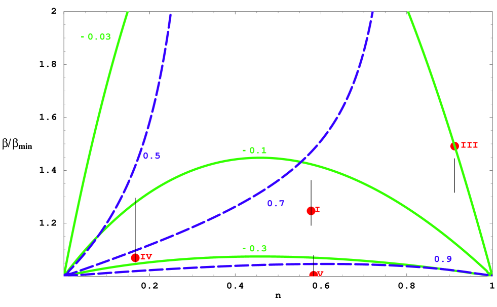
Figure 1: Four disk models of self-similar, gyrentropic accretion discussed in the text and located on the $n-\beta/\beta_{{\rm min}}$ plane assuming a fluid disk with $\eta=0,\gamma=5/3$. (Model II has $\gamma=4/3$; Model VI has large $\beta$.) The ordinate is the ratio of the scaled energy outflow to that required for a thin disk with $L=R^{1/2},B=-0.5/R$. The dashed lines are contours of constant $L/R^{1/2}$ in the case of 1D models and $\ell_{0}$ for 2D models; the solid lines are contours of constant $BR$ for 1D models and $b_{0}$ for 2D. The points correspond to the values of $\beta/\beta_{{\rm min}}$ for 1D models. The vertical lines passing upward through these points connect the equivalent values of $\beta/\beta_{{\rm min}}$ for circulation models to those for the outflow models (cf. Table 1). Using these and other measures, it can be shown that the 1D models provide a surprisingly good representation of the 2D models.

All				1D		2D	Circ.	Out.				Wind
No.	$\gamma$	$\ell_{0}$	$b_{0}$	$n$	$\beta$	$\theta_{d}$	$\beta$	$\beta$	$\eta$	$b_{d}$	$\theta_{w}$	$b_{w}$	$v_{\infty}$	$\theta_{j}$
I	1.67	0.75	-0.15	0.58	3.01	0.42	2.86	3.27	-0.10	-0.31	0.64	0.62	0.77	0.39
II	1.33	0.90	-0.20	0.58	3.12	0.60	2.87	3.26	-0.09	-0.30	0.91	0.59	0.89	0.39
III	1.67	0.75	-0.03	0.91	1.74	0.18	1.54	1.69	-0.03	-0.19	0.36	0.11	0.19	0.32
IV	1.67	0.75	-0.25	0.17	14.4	0.56	13.9	17.6	-0.76	-0.37	0.77	5.60	2.74	0.66
V	1.67	0.99	-0.46	0.58	2.38	1.34	2.33	2.59	-0.14	-0.49	1.40	0.55	1.13	1.34
VI	1.67	0.63	-0.02	0.58	10.0	0.11	7.05	8.25	-0.09	-0.11	0.34	0.78	0.47	0.24

Table 1: Physical parameters that characterise the six disk-outflow models, identified by Roman numerals. The models are described in four formalisms of increasing sophistication: a 1D model, a 2D gyrentropic model extending to zero pressure and density, the same with the internal circulation and convective heat flux computed self-consistently (Circ.), and a disk whose surface is chosen to be a thermal front that coincides with the base of the outflow (Out). The models are parametrised by the specific heat ratio $\gamma$, the equatorial Bernoulli function $b_{0}$ ($=RB$ for 1D models) and the scaled, equatorial angular momentum $\ell_{0}$ ($=R^{-1/2}L$ for 1D models). These parameters are sufficient to derive the mass loss exponent $n$ and the energy loss exponent $\beta$ in 1D, assuming that $\eta=0$. The basic 2D treatment adds a disk opening angle $\theta_{d}$. A viscous torque is introduced in the circulation models which modifies the derived energy loss rate. Further modifications to $\theta_{d},\beta,\eta$ occur in the outflow models. The scaled Bernoulli function changes from $b_{d}$ to $b_{w}$ on crossing the thermal front (at an angle $\theta_{w}$) in the outflow models. Asymptotically, the wind flows on the surface of an evacuated cone with scaled speed $v_{\infty}$ and opening angle $\theta_{j}$.

2.2.1 Model I: Fiducial, ion-supported disk

This reference model assumes that the hole is underfed so that the gas pressure is ion-dominated (with $\gamma=5/3$). We suppose that the gas has moderate pressure (parametrised by $B=-0.15/R$) and centrifugal support (parametrised by $L=0.75R^{1/2}$) and consequently moderate mass and energy loss rates ($n\sim 0.6,\beta\sim 3$).

2.2.2 Model II: Radiation-supported disk

Overfed, radiation-dominated accretion with $\gamma=4/3$. $L,B$ are chosen to give similar values of $n,\beta$ to Model I.

2.2.3 Model III: Thick disk

A much less bound version of Model I ($B\sim-0.03/R$) but with a similar circular velocity. The 2D disk is very thick with a small opening angle, $\theta\sim 0.2$. The mass loss rate is high ($n\sim 0.9$) and so the energy loss parameter is low ($\beta\sim 1.7$).

2.2.4 Model IV: Intermediate disk

A more tightly bound version of Model I ($B=-0.25/R$), with a somewhat thinner disk. The mass loss rate is relatively small ($n\sim 0.2$) and so $\beta\sim 14$ has to be correspondingly large to compensate.

2.2.5 Model V: Fast disk

A fast, thin disk ($L\sim 0.99R^{1/2}$). In order to create a model to explore this limit we choose to keep the mass loss rate index $n$ equal to that of Model I.

2.2.6 Model VI: Slow disk

A slowly rotating, thick disk ($L\sim 0.6R^{1/2}$), that is very weakly bound ($B\sim-0.02/R$), but with similar mass loss index to that of Model I. Again $\beta\sim 10$ is large.

3 Two-dimensional Disks

3.1 Høiland Criteria

In order to make a two-dimensional model of a slowly accreting and consequently hydrostatic disk, we must specify some relationship among the thermodynamical variables $P,{\cal P},S,$ etc. Our choice depends upon considerations of stability. An adiabatic, fluid accretion disk naturally develops a negative, radial entropy gradient as heat is generated in its interior. If rotation were unimportant, it would become unstable according to the Schwarzschild criterion. However, a Keplerian disk has a positive angular momentum gradient and, if we were to ignore entropy, it would be stable according to the Rayleigh criterion. For thin disks, the rotational stabilisation dominates the entropy destabilisation. However, for thick disks, the two effects must be compared directly.

To do this, consider a small, flat ribbon of fluid with an azimuthal length much greater than its width which, in turn, is much greater than its thickness. Let the ribbon undergo a displacement in the poloidal plane, parallel to its width. Assume that the motion is sufficiently slow that the ribbon remains in pressure equilibrium with its surroundings and sufficiently rapid that its entropy $S$ is unchanged (e.g.,  Goldreich & Schubert, 1967; Tassoul, 1978; Begelman & Meier, 1982). The net buoyant acceleration on the ribbon is then given by

$$\delta\vec{a}_{{\rm buoy}} = -(\delta\vec{r}\cdot\nabla)S\ \left({{\partial\ln{\cal P}\over\partial S}}\right)_{P}\left({\nabla P\over{\cal P}}\right)$$ (19)

$$= (\delta\vec{r}\cdot\nabla)S\ \nabla\left({P^{1-1/\gamma}\over 1-1/\gamma}\right),$$

where the spatial gradients are in the surrounding medium. If the displacement is also rapid enough for the ribbon’s specific angular momentum $L$ to be unchanged during the displacement, the surplus centrifugal acceleration of the ribbon relative to its surroundings is likewise given by

$$\delta\vec{a}_{{\rm cent}}=-(\delta\vec{r}\cdot\nabla)L^{2}\left({\vec{R}\over R^{4}}\right)=(\delta\vec{r}\cdot\nabla)L^{2}\nabla\left({1\over 2R^{2}}\right).$$ (20)

The total acceleration is the sum of equations (19) and (20).

If a virtual displacement $\delta\vec{r}$ is made, the virtual work done, per unit mass of fluid, is $\delta W=U_{ij}\delta r_{i}\delta r_{j}/2$, where the tensor ${\rm U}$ is given by

$${\rm U}=\nabla\left({P^{1-1/\gamma}\over 1-1/\gamma}\right)\otimes\nabla S+\nabla\left({1\over 2R^{2}}\right)\otimes\nabla L^{2}.$$ (21)

Only the symmetric part of ${\rm U}$ need be retained and we can rotate axes in the $r-\theta$ plane so that it is diagonal. The flow will be unstable if there exists a displacement $\delta\vec{r}$ such that $\delta W>0$. If the trace of ${\rm U}$ is positive, then there must be unstable displacements. This leads to the first Høiland instability condition,

$$\nabla\left({P^{1-1/\gamma}\over 1-1/\gamma}\right)\cdot\nabla S+\nabla\left({1\over 2R^{2}}\right)\cdot\nabla L^{2}>0.$$ (22)

Disks that satisfy this inequality are unstable in the equatorial plane to radial displacements. If we adopt our self-similar scalings and impose hydrostatic balance in the equatorial plane, then this instability condition can be re-written as

$$R^{3}\Omega^{2}<{3\gamma-5-2n\gamma+2n\over\gamma-5-2n\gamma+2n}\equiv a(\gamma,n).$$ (23)

For $\gamma=5/3\ (4/3)$, $a(\gamma,n)$ increases from $0\ (3/11)$ to $2/7\ (5/13)$ as $n$ increases from 0 to 1. It turns out that all of the 1- and 2-dimensional models discussed below strongly violate inequality (23). For this reason, we argue that adiabatic, fluid disks are quite stable to radial convection.

Nonetheless, when ${\rm Tr(U)}<0$, a second Høiland criterion must be considered and there will still be a range of unstable displacement directions if

$$\left[\nabla\left({P^{1-1/\gamma}\over 1-1/\gamma}\right)\times\nabla\left({1\over 2R^{2}}\right)\right]\cdot\left[\nabla S\times\nabla L^{2}\right]<0$$ (24)

or

$$(\nabla P\times\nabla R)\cdot(\nabla S\times\nabla L)>0.$$ (25)

In our application, the onset of instability is always associated with a change in sign of $\nabla S\times\nabla L$, not $\nabla P\times\nabla R$.

In order to interpret inequality (25), it is useful to define a series of 2D surfaces that are tangent on an equatorial ring lying in the disk midplane and on which $S,B,L,R,\Omega,r,P,{\cal P}$ are constant (Fig. 2). It is straightforward to show, by combining the Høiland criteria with the equation of hydrostatic equilibrium and its curl, that the surfaces of constant $S,L,B,R,\Omega,r,P,{\cal P}$, must be nested in order of increasing Gaussian curvature in a stable, fluid disk (Begelman & Meier, 1982; Blandford, Jaroszyński & Kumar, 1985). (Actually, it is not formally required that the “isorotes” [$\Omega=$ constant surfaces] be less curved than spheres, $r=$ constant, though this is true for all of our solutions.)

The surfaces on which the Bernoulli function $B$ is constant are particularly important. We call these “isoberns.” Using the equation of hydrostatic equilibrium, it can be shown that

$$\nabla B=H\nabla\ln S+\Omega\nabla L.$$ (26)

Equation (26) implies that the isoberns lie between the “isogyres” (surfaces of constant $L$) and the isentropes. Stability requires that the isogyres lie inside the isentropes (eq. [25]). When the disk is marginally stable, $S,L,B$ are constant on a common surface, which we call a “gyrentrope.” We argue that adiabatic, fluid disks should evolve quickly towards this state and we call such disks “gyrentropic” (cf.  Bardeen, 1973). In a marginally unstable disk, the growing eigenmodes have displacements that lie between the isentropes and the isogyres. In other words, near marginal stability, thin ribbons of gas move in opposite directions roughly along the nearly coincident isentrope/isogyre/isobern $=$ gyrentropic surfaces.

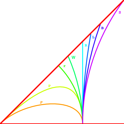
Figure 2: Structure of convectively-stable accretion disks. Level surfaces of density (${\cal P}$), pressure ($P$), spherical radius ($r$), angular frequency ($\Omega$), cylindrical radius ($R$), angular momentum ($L$), Bernoulli function ($B$) and entropy ($S$) passing through an equatorial ring of radius $r$. The configuration shown is dynamically stable according to both Høiland criteria eq. (25). When the order of the isentropes and isogyres is reversed, the flow becomes convectively unstable.

3.2 Numerical Simulations

There have been many simulations of fluid dynamical accretion disks, both two- and three-dimensional. In particular, Stone, Pringle & Begelman (1999) (SPB99) have carried out two-dimensional simulations of adiabatic disks evolving under a variety of prescriptions. Gas was supplied at an intermediate radius and endowed with viscosity. It spread inward (and outward) on a viscous timescale and became strongly convective, developing a gyrentropic structure at intermediate radii. Convection transported energy and angular momentum primarily along gyrentropes. In directions normal to the gyrentropes, the only means of transporting energy and angular momentum were via the viscous stress and advection. Since viscosity transports angular momentum outward with a positive divergence in the equatorial regions, the loss of angular momentum was balanced by a combination of meridional flow and convective transport of angular momentum between high latitudes and the equatorial region. When the gas was marginally unstable according to criterion eq. (25), convection exchanged mass, energy and angular momentum between the disk interior and high latitude and not radially outward throughout the disk.

The details of this balance between convection and circulation in the simulations depended upon the form of the viscous stress. For example, when the viscosity $\nu$ was set to be proportional to $\rho$ (Run B of SPB99), the viscous torque was balanced partially by inflow in the equatorial zones. But at high latitudes, where the gyrentropic surfaces themselves became roughly radial, the angular momentum flux was dominated by convective transport and the mass flux was generally outward, producing a quadrupolar flow pattern. When the viscosity was chosen to satisfy the self-similar scaling law, $\nu\propto r^{1/2}$, (Run K of SPB99), convection along gyrentropes was strikingly demonstrated in the cross-correlation of the entropy and the angular momentum (Fig. 3).

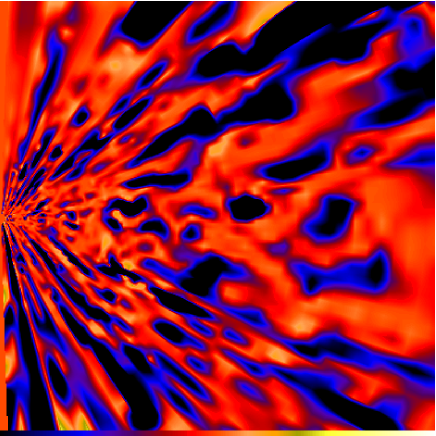
Figure 3: Cross-correlation of specific angular momentum and specific entropy from Run K of SPB99, showing convection along gyrentropic surfaces. A time-sequence of frames from this simulation shows both inflow and outflow of fluid elements parallel to these surfaces, particularly apparent at mid- and high latitudes.

SPB99 measured separately the radial mass inflow and outflow rates and found that they both obey $\dot{M}\propto r$ very roughly. The net mass accretion rate, given by the inflow rate minus the outflow rate, is approximately independent of $r$ and equals the inflow at the inner radius. In other words, the mass reaching the hole at $r_{{\rm in}}$ is a fraction $\sim(r_{{\rm in}}/r_{{\rm out}})$ of that supplied at $r_{{\rm out}}$. This is a strong indication that the flows had not become stationary which would probably require a continuous supply of gas at large radius.

3.3 Global Consequences of the Gyrentropic Hypothesis

We have argued, on the basis of the one-dimensional treatment, that a rotating flow will have $B>0$ unless there is some means of removing energy. We have also argued that such a flow will become convective and that the natural direction of energy transport is along gyrentropes, where $B$ is constant, to the disk surface. This strongly suggests that adiabatic, fluid disks lose energy though some form of outflow from their surfaces.

However, as emphasized by Abramowicz, Lasota & Igumenshchev (2000), the condition that $B>0$ somewhere does not automatically imply outflow. Consider a general, axisymmetric disk with surface described by the equation $r=r_{d}(\theta)$. As with a star, the surface properties of a disk can be quite subtle, but it is reasonable to suppose that the enthalpy at the top of the convection zone is much smaller than in the interior and can be ignored. In addition, the pressure will be small; consequently, the surface will be an isobar. Resolving the equation of motion along the disk surface, we obtain a differential equation that relates its shape to the variation of $B$ on the surface (and, indirectly, within the disk):

$${d\ln r_{d}\over d\ln\sin\theta}={-2(1+Br)\over 1+2Br}.$$ (27)

From the form of this equation, we discover that the disk surface can have $B>0$ provided that $d\ln\sin\theta/d\ln r_{d}<-1/2$, that is to say within a funnel where the cross section increases with height slower than parabolically. However, outside such a funnel, the surface must have $B<0$ if it is to remain bound. Indeed, when the disk latitude decreases with $r$, as it must eventually, then $-1<Br<-1/2$ must be satisfied along the free surface. Note, especially, that if the disk surface is conical, as it is in our similarity solutions, then

$$B(r,\theta_{d})={-1\over 2r}$$ (28)

over the entire surface.

The requirement that $B<0$ on the surface of a stable disk (excluding a funnel), however, is inconsistent with having $B>0$ in the interior. This is because the second Høiland criterion, eq. (25), requires that $B$ increase with altitude. It is for these reasons that we argue that conservative, adiabatic, fluid accretion disks do not exist and, instead, there must always be outflows.

3.4 Self-Similar, Gyrentropic Disks

We now present an elementary description of two-dimensional, self-similar, adiabatic, gyrentropic fluid disks. We shall make two key approximations in this description — that the only motion is rotational and that the disks are gyrentropic all the way to their surfaces where the density and pressure vanish simultaneously. Both of these approximations become accurate in the limit that the rate of dissipation tends to zero. In § 4, we shall introduce a prescription for relaxing the first of these and in § 5, we shall address the second.

In two dimensions, our assumption of self-similarity requires that the pressure, density and specific angular momentum satisfy the scalings:

$$P=r^{n-5/2}p(\theta),\ \ {\cal P}=r^{n-3/2}\rho(\theta),\ \ L=r^{1/2}\ell(\theta).$$ (29)

(Note that we consistently use upper case for the physical variables and lower case for their angular variations.)

The equations of motion are

$${1\over{\cal P}}{\partial P\over\partial r} = -{1\over r^{2}}+{L^{2}\csc^{2}\theta\over r^{3}}$$ (30)

$${1\over{\cal P}r}{\partial P\over\partial\theta} = {L^{2}\cot\theta\csc^{2}\theta\over r^{3}},$$ (31)

from which we obtain

$$(5/2-n)p/\rho = 1-\ell^{2}\csc^{2}\theta$$ (32)

$$p^{\prime}/\rho = \ell^{2}\cot\theta\csc^{2}\theta,$$ (33)

where the prime denotes differentiation with respect to $\theta$.

Now consider the entropy function

$$S=P^{1/\gamma}{\cal P}^{-1}=s(\theta)r^{{-a\over 1-a}},$$ (34)

where $a(\gamma,n)$ is defined in eq. (23) and $s=p^{1/\gamma}\rho^{-1}$.

Gyrentropicity implies that $S=S(L)$ and so self-similarity requires that

$$S\propto(r^{1/2}\ell)^{{-2a\over 1-a}}.$$ (35)

This provides an algebraic relation among $p$,$\rho$, and $\ell$.

The solution to equations (32), (33) and (35) is

$$\ell = \left\{a+[a^{2}+\ell_{0}^{2}(\ell_{0}^{2}-2a)\csc^{2}\theta]^{1/2}\right\}^{1/2}\sin\theta$$ (36)

$$p = \left({1-\ell^{2}\csc^{2}\theta\over 5/2-n}\right)^{\gamma\over\gamma-1}s^{-\gamma\over\gamma-1}$$ (37)

$$\rho = \left({1-\ell^{2}\csc^{2}\theta\over 5/2-n}\right)^{1\over\gamma-1}s^{-\gamma\over\gamma-1}$$ (38)

$$s = s_{0}\left({\ell\over\ell_{0}}\right)^{-2a\over 1-a}$$ (39)

where $\ell_{0}=\ell(\pi/2)$, etc., measures the angular momentum, etc., in the midplane at radius $r_{0}$. Equivalently, we can write

$$S=s_{0}\left({L\over\ell_{0}}\right)^{{-2a\over 1-a}}.$$ (40)

The disk terminates at a free surface where $p,\rho\rightarrow 0$ and so the disk opening angle is given by

$$\sin\theta_{d}=l_{d}=\ell_{0}\left({\ell_{0}^{2}-2a\over 1-2a}\right)^{1/2}.$$ (41)

We next use eq. (36) to solve for the gyrentropes, $L=$ const. These are given by

$$r=r_{L}(\theta)=r_{0}\ell_{0}^{2}/\ell^{2}.$$ (42)

The gyrentropes intersect the disk surface at a radius

$$r=r_{d}=r_{0}(1-2a)/(\ell_{0}^{2}-2a).$$ (43)

The Bernoulli function, which is also constant on gyrentropes, can be calculated using eq. (1) as

$$b=rB=-{\ell_{d}^{2}\over 2\ell^{2}},$$ (44)

consistent with eq. (40). Eq. (44) also allows us to relate the value of the Bernoulli function at the midplane ($\theta=\pi/2$) to the midplane angular momentum:

$$b_{0}=-{\ell_{0}^{2}-2a\over 2(1-2a)}.$$ (45)

Equivalent to eq. (40), we have

$$B=b_{0}\left({L\over\ell_{0}}\right)^{-2}.$$ (46)

The two autonomous relations, equations (40) and (46), are equivalent to the self-similar relation eq. (3) and the assumption of gyrentropicity and can be used to replace self-similarity when making a model of the inner disk (cf. § 6.2). Note that we are only free to specify two functional relations among $L,S,B$ because these relations must be consistent with the equations of motion, equations (30) and (31).

3.5 Two-Dimensional Gyrentropic Disk Models

For an assumed value of the specific heat ratio, $\gamma$, the above relations suffice to specify a two-parameter family of self-similar disk models. To facilitate comparison with the one-dimensional models, we choose these two additional parameters to be $R^{-1/2}L\rightarrow\ell_{0}$ and $RB\rightarrow b_{0}$. The mass loss exponent $n$ can then be thought of as being given implicitly by eq. (45), which is identical to the 1D relation, eq. (17). In addition, we must also specify the midplane entropy, $s_{0}$, which fixes the pressure and density. However, $s_{0}$ does not change the shape of either the disk or the isogyres and can be set to unity without loss of generality.

The six two-dimensional models, corresponding to the six illustrative one-dimensional models (§ 2.2), are exhibited in Fig. 4. These models demonstrate that the gyrentropes are generically negatively curved surfaces, implying that the isorotes (surfaces of constant $\Omega$) are positively curved. They also show that the disks thicken, for a given equatorial angular momentum $\ell_{0}$, as the mass loss rate, measured by $n$, decreases. Conversely, for a given value of $n$, the disks thicken as the rotational support, measured by $\ell_{0}$, decreases and the pressure becomes more important. Observe that changing the specific heat ratio is relatively unimportant. In this way, adiabatic accretion is rather different from spherical accretion, where $\gamma=5/3$ constitutes a singular limit.

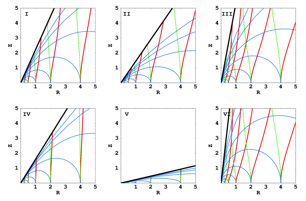
Figure 4: The six simple 2D disk models described in § 3.5 and Table 1. The isobars, isorotes and gyrentropes are shown with dotted, dashed and solid contours, respectively. In these models, it is assumed that convection is efficient and extends all the way to the disk surface. The outflow does not influence the disk structure in these models.

4 Circulation Disks

4.1 Energy and Angular Momentum Transport

We have so far treated the disk as being in circular motion and strictly gyrentropic. We now relax the first of these assumptions. Suppose that there is a local torque per unit length

$$G\equiv{d\dot{M}{\cal G}\over ds}$$ (47)

(where $ds$ is an element of length in the meridional plane), that is small enough that we can treat its effect as perturbative upon the fundamental, gyrentropic flow pattern. (Note that $G$ is integrated over azimuth.) We conjecture that this torque will eventually drive a fluid disk to marginal instability everywhere, so that the isentropes lie just “inside” the isogyres and that, except near the disk surfaces, we can continue to approximate the disk angular momentum distribution as gyrentropic.

As was discussed in § 3.1, the convective motions consist of slender ribbons of fluid moving between these two surfaces. We suppose that the angle between the isogyres and isentropes will open up just enough to allow the relevant transport to take place. Heat and angular momentum can be convected in this manner as a displaced ribbon can exchange both quantities with its surroundings. The relative efficiency with which this happens will depend upon the effective Prandtl number, $Pr$. We assume that the local thermal conductivity is much higher than the local effective viscosity, implying that $Pr$ is large and that the meridional flow is driven by the torque as opposed to thermal conduction. It then follows that the displacements will nearly follow the isogyres and that the convective transport of heat $Q$ will be more important than the convective transport of angular momentum, because the ribbons develop larger departures from local thermal than mechanical equilibrium. We will consequently ignore convective angular momentum transport and suppose that the only torque is Newtonian, i.e., $G\propto-\nabla\Omega$. (Alternative prescriptions are certainly possible and we shall consider some in the following paper. However, we contend that our prescription is the natural choice for high $Pr$, fluid disks.)

Convection, along gyrentropes, involves relatively rapid, forward and backward motions that average to give a net mass flux per unit length parallel to the gyrentropes, after integrating in azimuth. To this must be added the steady inflow (or outflow) of the gas perpendicular to the gyrentropes. The two flows are combined into a single poloidal mass current vector

$$\vec{J}=2\pi R{\cal P}\vec{V}_{p}=r^{n-1}\vec{j}(\theta)$$ (48)

where $\vec{V}_{p}\equiv[V_{r},V_{\theta}]$.

4.2 Torque Density

Consistent with the preceding discussion, we write

$$\vec{G} \equiv r^{n-1/2}\vec{g}(\theta)$$ (49)

$$= -2\pi\alpha R^{3}P\nabla\ln\Omega$$ (50)

$$= 3\pi\alpha\sin^{3}\theta p[1,-2\omega^{\prime}/3\omega]r^{n-1/2}$$ (51)

where $\omega=r^{3/2}\Omega=\ell\csc^{2}\theta$ is the scaled angular velocity, $\alpha\equiv\nu{\cal P}\Omega/P$ is the standard viscosity parameter (Shakura & Sunyaev, 1973) and $\nu$ is the kinematic viscosity. $\vec{G}$ can be treated as a poloidal vector in this approximation although it is really a third rank tensor. In order to comply with our self-similar assumption, we set $\alpha=$ constant. This ensures that the characteristic inflow and circulation speeds are fixed fractions ($\propto\alpha$) of the Keplerian value.

4.3 Conservation Laws

We can now write down equations representing the conservation of mass and angular momentum:

$$\nabla\cdot\vec{J}=0;\qquad\nabla\cdot(L\vec{J}+\vec{G})=0.$$ (52)

Adopting our self-similar prescription, these equations combine to give two ordinary differential equations,

$$j_{\theta}^{\prime}={2n\over\ell}[\ell^{\prime}j_{\theta}+(n+{1\over 2})g_{r}+g_{\theta}^{\prime}]=-nj_{r}.$$ (53)

This can be solved for an assumed value of $n$ subject to the boundary condition $j_{\theta}(\pi/2)=0$. Note that solutions to this equation automatically conserve mass. If we start by assuming that $\dot{M}\propto r^{n}$, then the net mass flowing across a hemispherical surface, $\dot{M}=-r\int_{\theta_{d}}^{\pi/2}d\theta J_{r}$, automatically satisfies $d\dot{M}/dr=-J_{\theta}(\theta_{d})$, as required. The solutions for the flow and the torque (Fig. 5) show that there is a net inflow across the gyrentropes and that the total mass inflow at a given radius in a disk of given shape satisfies $\dot{M}\propto s_{0}^{-\gamma/(\gamma-1)}\alpha$.

However, superimposed upon this inflow is a quadrupolar circulation, directed inward in the equatorial region and outward near the disk surface. In some, though not all, solutions the combined, radial flow is outward at high latitude.

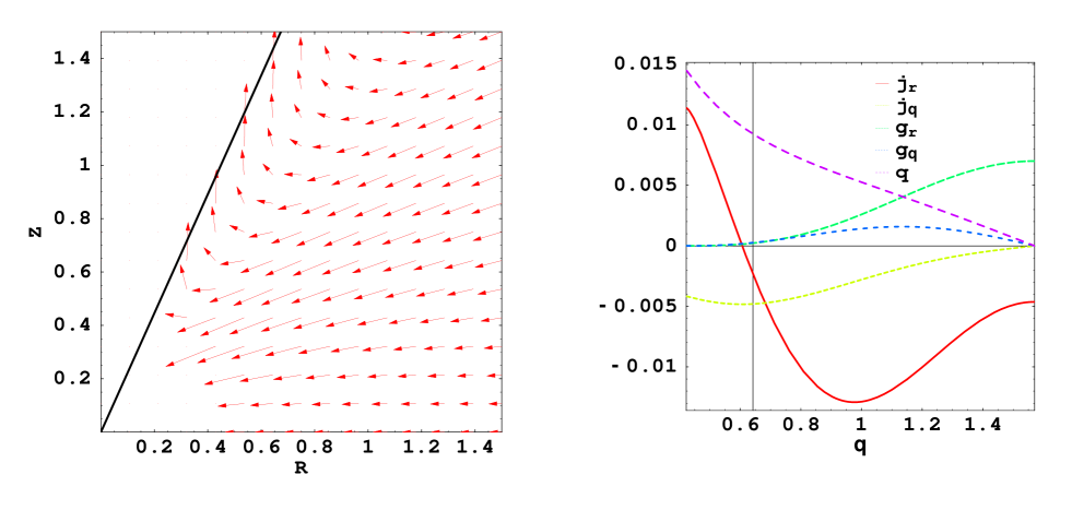
Figure 5: Circulation model for the fiducial illustrative example I. a) Poloidal mass flux $\vec{j}$ from eq. (53). It is assumed that the mass flow extends all the way to the disk surface. Note that, although the net poloidal flow is inward, the flow is actually outward near the disk surface. b) The two components of the mass flux $\vec{j}$ and the assumed viscous torque $\vec{g}$, as well as the convective heat flow along the gyrentropes, measured by $q$. The vertical line marks the location of the thermal front in the outflow model (cf. § 5).

Although the solution for $\vec{J}$ is finite at the disk surface, the velocity $\vec{V}=\vec{J}/2\pi R{\cal P}$ diverges. This signals the failure of our model for convective energy transport, as we discuss in the following section. By contrast, the torque density $\vec{G}$ vanishes at the disk surface according to eq. (49). The angular momentum incident on the disk surface is then

$${dF_{L}\over dr}=-LJ_{\theta}=L{d\dot{M}\over dr}\Rightarrow\eta=0,$$ (54)

where we have used eq. (6). This confirms that the outflowing gas only carries off its own specific angular momentum, cf. eq. (7), BB99.

We next solve for the convective energy flux $\vec{Q}$. This must be directed along the gyrentropes and so we can write it in the form

$$\vec{Q}\equiv[2\ell^{\prime},-\ell]\ q(\theta)r^{n-2}.$$ (55)

The equation of energy conservation becomes

$$\nabla\cdot[B\vec{J}+\Omega\vec{G}+\vec{Q}]=0.$$ (56)

This furnishes a first order differential equation for $q(\theta)$,

$$\ell q^{\prime}-(2n-3)\ell^{\prime}q+j_{r}b-j_{\theta}b^{\prime}-(n-1)\omega g_{r}-\omega^{\prime}g_{\theta}-\omega g_{\theta}^{\prime}=0,$$ (57)

which can be solved subject to $q(\pi/2)=0$.

The supply of energy to the disk surface is given by

$${dF_{E}\over dr}=J_{\theta}B+Q_{\theta}.$$ (58)

Comparing with eq. (9) we deduce that

$$\beta={Q_{\theta}\over J_{\theta}B}={\ell_{d}q_{d}\over j_{\theta d}b_{d}}={-2\sin\theta_{d}q_{d}\over j_{\theta d}}$$ (59)

where $\ell_{d},b_{d}$ are given by equations (41) and (28) and $j_{\theta d},q_{d}$ are given by solutions of the differential equations (53) and (57). $\beta$ is then a function of $\ell_{0}$, $n$ and, implicitly of $\ell_{0}$, $b_{0}$ as in the 1D models.

In the important limit when the disk expands all the way to the pole, with $\theta_{d},\ell_{d}\rightarrow 0$ and $\ell_{0}\rightarrow(2a)^{1/2},\ b_{0}\rightarrow 1/2$, then $\beta\rightarrow\infty$.

4.4 Circulation Disk Models

We have computed circulation disk models corresponding to the 1D, 2D models discussed in § 2.2, § 3.5. In Fig. (5), we exhibit the flow pattern for our fiducial Model I (adopting a viscosity parameter $\alpha=0.03$). We also present the angular variations of the mass flux, torque and convective heat flux. The poloidal flow is fundamentally quadrupolar, inward at low latitude and outward at high latitude. The flows for the other five circulation models are qualitatively similar.

5 Outflow Disks

5.1 Efficiency of Convection

We now turn to the second of our modifications to the basic gyrentropic disk model, which introduces features that may be largely absent from existing numerical simulations due to inadequate resolution and/or missing physical processes. We allow for the fact that convection of energy and angular momentum will not be efficient close to the disk surface so that the gyrentropic approximation may no longer hold. We have already argued that the convection will be along the isogyres. Assuming that the isogyres and the isentropes have the unstable ordering with an angle $\delta$ between them, then, according to standard mixing-length theory (e.g.,  Hansen & Kawaler, 1994), the convective energy flux, integrated over azimuth, will be given by

$$Q \sim 2\pi R{\cal P}v_{c}^{3}$$ (60)

$$\sim 2\pi RP^{3/2}{\cal P}^{-1/2}(\vec{h}_{P}\cdot\nabla\ln S)^{3/2}$$ (61)

$$\sim 2\pi RP^{3/2}{\cal P}^{-1/2}\delta^{3/2}$$ (62)

where $v_{c}$ is the convection speed and $\vec{h}_{P}$ is a vector of length equal to the pressure scale height and tangent to the isogyre. (We drop numerical constants of order unity.) The Mach number of the convective motions is given by

$$M_{c}\sim\delta^{1/2}\sim\left({Q{\cal P}^{1/2}\over 2\pi RP^{3/2}}\right)^{1/3}\sim\left({q\ell\rho^{1/2}\over 2\pi p^{3/2}\sin\theta}\right)^{1/3}.$$ (63)

5.2 Thermal Front

We now make the ansatz that, when $M_{c}$ reaches a certain critical value $M_{c,crit}$, which we choose, arbitrarily, though not unreasonably, to be unity, the convective motions rapidly dissipate and the convective energy flux is quickly converted into heat, increasing the entropy of the gas. Simultaneously, we suppose that the torque ceases to act and that the viscous transport of angular momentum and energy stops abruptly. In reality, this transition is likely to occur gradually through the dissipation of turbulent wave modes and the acceleration of the flow within an extended region. However, approximating this transition as a discontinuity, located at a biconical thermal front, suffices for us to make a simple model.

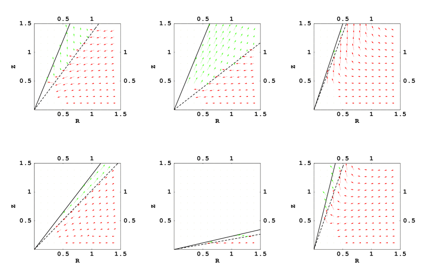
Figure 6: Poloidal flows for the six outflow disk models listed in § 2.2 and Table 1. Within the disk, the conditions are identical to those presented in Fig. 5. However, the disk is presumed to terminate at a thermal front (with opening angle $\theta_{w}$; dashed line) where the convective heat flux and the viscosity abruptly vanish and across which the flows of mass, momentum and energy are conserved. This is where the outflow begins (cf. § 5.2). The outflow lies between cones with opening angles $\theta_{j},\theta_{w}$. The flow at small radius is omitted.

We impose jump conditions at this transition by requiring that the mass, momentum and energy fluxes are equal on either side of the transition.

$$[J_{\theta}] = 0\Rightarrow j_{\theta w}=j_{\theta,th}$$ (64)

$$\left[J_{\theta}V_{r}\right] = 0\Rightarrow v_{r,w}=v_{r,th}$$ (65)

$$\left[2\pi RP+J_{\theta}V_{\theta}\right] = 0$$

$$\Rightarrow j_{\theta,th}(v_{\theta,w}-v_{\theta,th}) = 2\pi\sin\theta_{w}(p_{th}-p_{w})$$ (66)

$$\left[G_{\theta}+J_{\theta}L\right] = 0\Rightarrow j_{\theta,th}(\ell_{w}-\ell_{th})=g_{\theta,th}$$ (67)

$$\left[G_{\theta}\Omega+J_{\theta}B+Q_{\theta}\right] = 0$$

$$\Rightarrow j_{\theta,th}(b_{th}-b_{w}) = \ell_{th}q_{th}-g_{\theta,th}\omega_{th}.$$ (68)

These equations allow us to solve for the initial physical conditions (specifically $p_{w},\rho_{w},\vec{v}_{w}$) at the base of the wind (designated $w$) in terms of those upstream from the thermal front (designated $th$). The disk now terminates at an opening angle $\theta_{w}$ rather than $\theta_{d}$ and equations (54) and (59) must be replaced with

$$\eta = {g_{\theta,th}\over\ell_{th}j_{\theta,th}}$$ (69)

$$\beta = {\ell_{th}q_{th}-g_{\theta,th}\omega_{th}\over j_{\theta,th}b_{th}}.$$ (70)

Note that $\eta$ will now be negative because the isorotes are less curved than spheres. This is an artificial consequence of locating the effective disk surface inside the disk. In general, $\eta$ is usually small for fluid disks and it is a fair approximation to ignore it.

5.3 Wind Solutions

We now turn to the structure of a thermally-driven, gas dynamical wind and describe simple similarity solutions along the lines of those first derived by Bardeen & Berger (1978). We suppose that a gas dynamical wind is launched from the surface of the disk located at $\theta=\theta_{w}$ with initial conditions determined by the jump conditions at the thermal front. In the solutions that we shall consider, the increase in entropy at the thermal front is sufficient to change the sign of the Bernoulli function and render the gas unbound. We suppose that in its subsequent flow we can ignore viscous stress and mixing of mass, angular momentum and energy between streamlines.

We continue to adopt the self-similar scalings and generalize the velocity to a three-dimensional vector,

$$\vec{V}=r^{-1/2}[v_{r}(\theta),v_{\theta}(\theta),v_{\phi}(\theta)],$$ (71)

in spherical polar coordinates. The equations of continuity, motion and entropy conservation can be written:

$${\rho^{\prime}\over\rho}+{v_{\theta}^{\prime}\over v_{\theta}}=-\cot\theta-{nv_{r}\over v_{\theta}}$$ (72)

$${v_{r}^{\prime}\over v_{r}}={(v_{r}^{2}+2v_{\theta}^{2}+2v_{\phi}^{2}-2)\rho+(5-2n)p\over 2\rho v_{r}v_{\theta}}$$ (76)

$${v_{\theta}^{\prime}\over v_{\theta}}+\left({p\over\rho v_{\theta}^{2}}\right){p^{\prime}\over p}={2v_{\phi}^{2}\cot\theta-v_{r}v_{\theta}\over 2v_{\theta}^{2}}$$

$${v_{\phi}^{\prime}\over v_{\phi}}=-{v_{r}\over 2v_{\theta}}-\cot\theta$$

$${1\over\gamma}{p^{\prime}\over p}-{\rho^{\prime}\over\rho}=\left({a\over 1-a}\right){v_{r}\over v_{\theta}}$$

where a prime denotes differentiation with respect to $\theta$.

These equations can now be rearranged:

$$p^{\prime} = \gamma p\rho[(1+2n(a-1)+a)v_{r}v_{\theta}$$ (77)

$${\qquad\qquad+2(a-1)(v_{\phi}^{2}+v_{\theta}^{2})\cot\theta]\over\qquad 2(a-1)(\gamma p-\rho v_{\theta}^{2})}$$

$$\rho^{\prime} = -\rho[v_{r}(2\gamma pa+(2n-1)(a-1)\rho v_{\theta}^{2})$$ (78)

$${\qquad\qquad+2(a-1)\rho v_{\theta}(v_{\phi}^{2}+v_{\theta}^{2})\cot\theta]\over\qquad 2(1-a)v_{\theta}(\gamma p-\rho v_{\theta}^{2})}$$

$$v_{r}^{\prime} = {(5-2n)p+\rho(2v_{\phi}^{2}+v_{r}^{2}+2v_{\theta}^{2}-2)\over 2\rho v_{\theta}}$$ (79)

$$v_{\theta}^{\prime} = [v_{r}(-2\gamma p(a+na-n)+(a-1)\rho v_{\theta}^{2})$$ (80)

$${\qquad\qquad-2(a-1)(\gamma p+\rho v_{\phi}^{2})v_{\theta}\cot\theta]\over\qquad 2(a-1)(\gamma p-\rho v_{\theta}^{2})}$$

$$v_{\phi}^{\prime} = {-v_{\phi}(v_{r}+2v_{\theta}\cot\theta)\over 2v_{\theta}}\ .$$ (81)

These equations have three integrals, as may be readily verified. The entropy $S$, the Bernoulli function $B$ and the specific angular momentum $L$ are conserved along streamlines. We conclude that, as with the disk, $S=S(L),B=B(L)$ in the wind, although for a quite different reason. The entire flow can then be labeled using the disk gyrentropes that extend out to the thermal front where they are replaced by the wind gyrentropes.

Now consider the wind flow well away from the disk. There is potentially a critical point where $v_{\theta}=(\gamma p/\rho)^{1/2}$, the adiabatic sound speed. (The reason why only the $\theta$ component of the velocity is involved is that self-similarity and axisymmetry prescribe the other two components.) However, solutions satisfying appropriate boundary conditions never reach their critical speeds. From a mathematical point of view, these winds are “breezes,” and $v_{\theta}$ is always subsonic, even if the radial velocity becomes strongly supersonic. (In fact, $v_{\theta}$ must be subsonic, under all conditions, for $\gamma<3/2$.)

As $B$ is conserved in the outflow we can use its value at the thermal front to compute the asymptotic wind speed. We express the speed, $v_{\infty}$, by tracing the flow back to the thermal front on a flow line and then back to the midplane on a gyrentrope. $v_{\infty}$ is then given in Table 1 in units of the Keplerian speed at this point.

5.4 Outflow Disk Models

We have integrated equations (77)–(81) and produced matched flows for the six examples (Fig. 6). We find that it is generally possible to obtain physically plausible solutions for viable disk models. For each of our examples, which span a much larger volume of parameter space than we envisage is occupied by real disks, we find that the viscous dissipation creates so much heat that it easily unbinds the gas downwind of the thermal front. The outflow always occupies a hollow cone on account of the centrifugal barrier. The computed thermal fronts lie somewhat below the surfaces of the computed 2D disks (i.e. , $\theta_{w}>\theta_{d}$) and so the outflow disks are somewhat thinner than the equivalent circulation disks, but not by a large factor for reasonable values of $\alpha$ and $M_{c,crit}$. The jet cones have angles $\theta_{j}$ that are not much smaller than the thermal front cone angles, $\theta_{w}$. The values of $\beta$ computed in these more complete models do not differ greatly from those in our simple 1D and circulation disk models. The values of the angular momentum loss parameter $\eta$ are generally small except for Model IV, where it is compensating for the low mass loss rate.

We have made a very simple, two-part model to account for the dissipation. We suppose that there is distributed, Newtonian dissipation within the disk, and a discontinuous entropy production front at the disk surface. How do our results depend upon the choice of $\alpha$, which controls the former process, and $M_{c,crit}$, which controls the latter? For Model I, we find that increasing $\alpha$ from 0.03 to 0.1 causes the thermal front to be located at greater density in the disk, where the opening angle is $\theta_{w}=0.78$ as opposed to 0.64. The cone excluded by the jet has a correspondingly larger opening angle, increasing to $\theta_{j}=0.46$ from 0.39. Conversely, when we reduce $\alpha$ to 0.01, the thermal front is located at $\theta_{w}=0.57$, i.e., closer to the surface of the original gyrentropic disk at $\theta_{d}=0.42$, so that the original gyrentropic model becomes more accurate. (In addition, $\theta_{j}$ falls to 0.33.)

When we separately reduce $M_{c,crit}$ to 0.7 we find that the thermal front is located deeper in the disk, at $\theta_{w}=0.76$, and that the jet cone angle increases to $\theta_{j}=0.55$ as the outflow is launched with a lower speed relative to the surface of the thermal front. Our models are therefore not strongly sensitive to the values of $\alpha$ and $M_{c,ccrit}$, and the sense of the changes that variations in these parameters bring about are as expected.

6 Non-self-similar Flow at Small and Large Radii

6.1 Energy Release in Adiabatic Flows

We have so far concentrated upon self-similar models of adiabatic accretion flows because these allow us to generate self-consistent solutions through solving ordinary differential equations. However, as was made clear in BB99, the requirement that energy be carried away somehow from an adiabatic flow follows from general conservation laws and is not dependent upon self-similarity. If, for example, the viscous torque were to decrease suddenly at the radius where the disk becomes neutral, the thickness and the outflow would also be expected to exhibit abrupt changes. However there would still be a need for the energy released at small radius to be carried off in an outflow. In the context of the present paper, the disks should still convect energy to their surfaces and drive meridional circulation.

Furthermore, self-similar solutions cannot describe important features of the flow at small and large radius where self-similarity must fail. In this section, we discuss relativistic flow at small radius and non-self-similar flow near the outer transition radius.

6.2 Relativistic Flow at Small Radius

A convenient form of the equation of hydrostatic balance for a stationary, axisymmetric flow is

$$-{\nabla P\over\tilde{\cal P}\tilde{H}}=\vec{\tilde{A}}=\nabla\ln\tilde{E}-{\tilde{\Omega}\nabla\tilde{L}\over 1-\tilde{\Omega}\tilde{L}}$$ (82)

where $c=1$, $\vec{\tilde{A}}$ is the acceleration and the relativistic enthalpy per unit rest mass is $\tilde{H}=1+H=1+\gamma P/(\gamma-1)\tilde{\cal P}$, with $\tilde{\cal P}$ now representing the proper density of rest mass. This applies to both radiation-dominated ($\gamma=4/3$) and ion-dominated ($\gamma=5/3$) flows. $\tilde{E}=-u_{0}$ is the energy at infinity, $\tilde{\Omega}=u^{\phi}/u^{0}$ is the angular velocity and $\tilde{L}=-u_{\phi}/u_{0}$ is the fluid angular momentum. [Note that the relativistic definition of angular momentum differs from the conventional dynamical choice of $u_{\phi}$. It is more convenient for fluid dynamical use (Bardeen, 1973; Seguin, 1975).] These essentially kinematical quantities are related through

$$\tilde{E}(r,\theta,\tilde{L}) = (-g^{00}+2g^{0\phi}\tilde{L}-g^{\phi\phi}\tilde{L}^{2})^{-1/2}$$ (83)

$$\tilde{\Omega}(r,\theta,\tilde{L}) = {g^{0\phi}-g^{\phi\phi}\tilde{L}\over g^{00}-g^{0\phi}\tilde{L}}.$$ (84)

where $g^{\alpha\beta}$ is the contravariant form of the metric tensor in Boyer-Lindquist coordinates for a hole with specific angular momentum $a$. For illustration we adopt the value $a=0.95m$.

The relativistic generalization of eq. (26) is

$$\nabla\ln\tilde{B}=(1-\tilde{H}^{-1})\nabla\ln S+{\tilde{\Omega}\nabla\tilde{L}\over 1-\tilde{\Omega}\tilde{L}},$$ (85)

where

$$\tilde{B}=\tilde{H}\tilde{E}$$ (86)

is the relativistic Bernoulli function and the entropy function is still given by eq. (2). Note that the Bernoulli function now includes a contribution from the rest mass.

The two non-relativistic Høiland criteria, equations (22) and (25), have relativistic counterparts (Seguin, 1975; Blandford, Jaroszyński & Kumar, 1985). The first criterion for marginal instability generalizes to become:

$${1\over\tilde{H}^{2}}\nabla\left({P^{1-1/\gamma}\over 1-1/\gamma}\right)\cdot\nabla S-\vec{\gamma}\cdot\nabla\tilde{L}>0$$ (87)

where

$$\vec{\gamma}={d\vec{\tilde{A}}\over d\tilde{L}}={E^{4}\nabla\tilde{L}\over g_{0\phi}^{2}-g_{00}g_{\phi\phi}}-{\nabla\tilde{\Omega}\over(1-\tilde{\Omega}\tilde{L})^{2}}$$ (88)

and the derivative is performed assuming only circular motion. The second criterion also generalizes to become

$$(\nabla P\times\vec{\gamma})\cdot(\nabla S\times\nabla\tilde{L})>0.$$ (89)

We find that the first Høiland criterion is even more strongly satisfied in the inner disk (where the entropy gradient changes to become stabilizing) than in the self-similar disk. We conjecture that the flow will evolve to a state of marginal stability according to the second Høiland criterion so that the entire disk is gyrentropic.

In order to construct a gyrentropic inner disk model, we need to introduce two autonomous functions $S(\tilde{L}),\tilde{B}(\tilde{L})$ as described in § 3.4. What we actually do is ultimately equivalent. We specify equatorial distributions of angular momentum and entropy, $\tilde{L}(r_{0}),\tilde{S}(r_{0})$, from which we can deduce $\tilde{S}(\tilde{L})$, that are chosen to match onto the non-relativistic functions at large radius. In addition, the angular momentum must equal the relativistic Keplerian value at two radii — a radius $r_{m}$ where the pressure is maximized and a smaller radius $r_{c}$ (the “cusp” radius) where the pressure and its gradient vanish. The particular form of $\tilde{L}$ that we use is

$$\tilde{L}(r_{0})=\ell_{0}r_{0}^{1/2}[1+c_{1}\exp(-c_{2}r_{0})]$$ (90)

where the constants $c_{1}=1.78,$, $c_{2}=0.18$ are chosen to fit a disk with $r_{c}=1.84m$, $r_{m}=6m$ (Fig. 7).

The entropy function is required to satisfy the first Høiland criterion and has to be tuned to allow the Bernoulli function, derived below, to match the non-relativistic form $B(r_{0})=b_{0}r_{0}^{-1}$ at large radius. We use

$$S(r_{0})=r_{0}^{-a\over 1-a}[1+c_{3}\exp(-c_{4}r_{0})].$$ (91)

The choices $c_{3}=5.0,c_{4}=0.85$ produce a suitable solution.

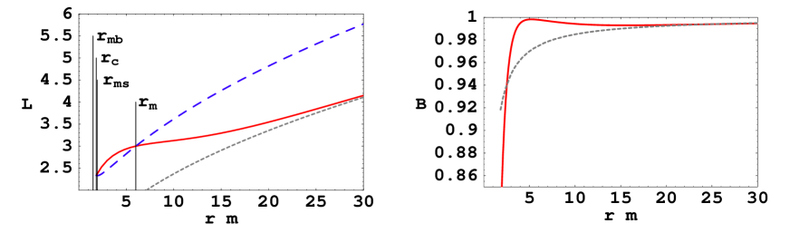
Figure 7: a) Assumed relativistic, fluid angular momentum variation, $\tilde{L}$ (solid) for a gyrentropic disk around a Kerr hole with $a=0.9m$. The Keplerian variation (dashed) is shown for comparison. The two angular momenta must coincide at the cusp radius $r_{c}=1.84m$ and at the pressure maximum at $r_{m}=6m$. At large radius the fluid angular momentum asymptotes to the Model I self-similar solution (dotted). Also shown are the radius of zero binding energy $r_{mb}=1.5m$ and the radius of marginal stability $r_{ms}=1.93m$. b) Derived variation of the relativistic Bernoulli function $\tilde{B}(r_{0})$ (dashed). Like the entropy, it asymptotes quickly to the non-relativistic form $B(r_{0})=b_{0}r_{0}^{-1}$.

In order to compute the Bernoulli function, we use eq. (83) to compute the energy $\tilde{E}$ and the angular velocity $\tilde{\Omega}$ as functions of equatorial radius $r_{0}$. We then rewrite eq. (85) in the form

$${d\tilde{B}\over dr_{0}}=(\tilde{B}-\tilde{E}(r_{0})){d\ln S\over dr_{0}}(r_{0})+{\tilde{\Omega}(r_{0})\tilde{B}\over 1-\Omega(r_{0})\tilde{L}(r_{0})}{d\tilde{L}\over dr_{0}}$$ (92)

and solve this differential equation to infer the variation $\tilde{B}(r_{0})$ and, consequently, $\tilde{B}(\tilde{L})$ (Fig. 7).

The next step is to solve for the disk structure away from the equatorial plane. Again we use eq. (85), this time written in the form:

$${d\tilde{B}\over d\tilde{L}}(\tilde{L})=(\tilde{B}(\tilde{L})-\tilde{E}(r,\theta,\tilde{L})){d\ln S\over d\tilde{L}}(\tilde{L})+{\tilde{\Omega}(r,\theta,\tilde{L})\tilde{B}(\tilde{L})\over 1-\Omega(r,\theta,\tilde{L})\tilde{L}}$$ (93)

and solve this for $\tilde{L}(r,\theta)$. This enables us to calculate $S(r,\theta),B(r,\theta)$ and then to compute $E(r,\theta),\Omega(r,\theta)$ using eq. (83). Finally, we can calculate the pressure using

$$P=\left[\left({\gamma-1\over\gamma S}\right)\left({\tilde{B}-\tilde{E}\over\tilde{E}}\right)\right]^{\gamma\over\gamma-1}$$ (94)

and plot the isobars (Fig. 8).

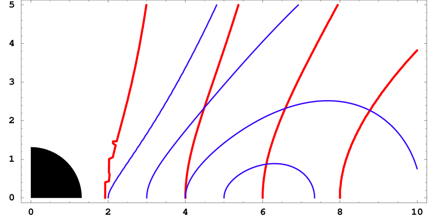
Figure 8: Model of the inner regions of gyrentropic accretion disk orbiting a Kerr black hole with the assumed angular momentum and entropy distributions displayed in Fig. 7. The gyrentropes are displayed as bold contours. The cusp is located between the marginally bound and marginally stable orbits. The isobars are shown as light contours surrounding the pressure maximum.

Although our choice of functions in equations (90) and (91) is arbitrary and has no immediate physical basis, our procedure does illustrate how to construct self-consistent disk models given a more comprehensive theory of relativistic convection. It is straightforward, in principle, to generalize the non-relativistic, self-similar development of circulation and outflow disk models to the non-self-similar regime. We could use the relativistic generalizations of equations (52) and (56) to derive partial differential equations for the poloidal velocity for a non-self-similar circulation and outflow. However, there is little point in carrying out this exercise as the assumed autonomous relations that define the gyrentropes are arbitrarily prescribed. It is, instead, more valuable to solve the time-dependent 2D and 3D fluid dynamical equations numerically, making different assumptions about the viscosity and, perhaps, the heat transport. The principles that we have developed here should be of use in interpreting such a computation.

6.3 Transition Disk

Self-similarity must also break down at some outer radius, which either represents an outer boundary condition associated with the mass supply or the radius beyond which radiative losses are significant. In the ion-dominated case, cooling near the outer transition radius $r_{t}$ (i.e., between a thin radiative disk and an ADIOS) is likely to be dominated by thermal bremsstrahlung of the one-temperature ($T_{e}=T_{i}$) plasma, provided that $r_{t}>2000m$ (where $m=GM/c^{2}$ is the gravitational radius). Equating the cooling rate and the inflow time, we find that adiabatic flow is possible for

$$r_{t}<10^{9}{\alpha^{4}\over\dot{m}_{t}^{2}}m,$$ (95)

where $\dot{m}_{t}\equiv\dot{M}_{t}/\dot{M}_{E}$ is the mass flux crossing into the nonradiative region (the mass supply). Given a power-law scaling of $\dot{m}$ with index $n$ at $r<r_{t}$, the mass flux reaching the black hole (the accretion rate) is

$$\dot{m}_{\rm acc}<10^{-9n}\alpha^{-4n}\dot{m}_{t}^{1+2n}.$$ (96)

For example, if $\dot{m}_{t}=0.01$, $\alpha=0.03$ and $n=0.6$ (as in Model I), the accretion rate can be as low as $\dot{m}_{\rm acc}\sim 10^{-6}$, four orders of magnitude lower than the supply rate. Since $\dot{m}_{\rm acc}\ll 50\alpha^{2}\sim 0.05$, the ADIOS easily satisfies the condition for a two-temperature flow close to the black hole (Rees et al., 1982) — which is more stringent than the condition for adiabatic flow at large radii — implying that the adiabatic flow, once established, will extend all the way from $r_{t}$ in the vicinity of the hole. For conservative inflow models, this condition is more difficult to satisfy. Moreover, for the parameters we have chosen $r_{t}$ can be as large as $\sim 10^{7}m$; thus the flow could exhibit self-similarity over several decades in radius.

Similar considerations apply to accretion flows with $\dot{m}\gg 1$. Here the transition from radiative to nonradiative flow occurs at the trapping radius, $r_{t}\sim r_{\rm trap}\sim\dot{m}_{t}m$ (Begelman, 1979). The accretion rate is given by $\dot{m}_{\rm acc}\sim\dot{m}_{t}^{1-n}$.

We note that models for the transition between the thin disk and nonradiative flow have been studied mainly in the context of ADAF models, in which conserved mass flux through the disk is assumed (e.g.,  Kato & Nakamura, 1998; Manmoto et al., 2000). These models generally require a zone of anomalous emissivity near $r_{t}$ in order to soak up the outward energy flux, which cannot be accepted by the thin disk in a smooth transition. This problem is avoided if we allow for the onset of mass (and angular momentum) loss in the transition region.

In order to demonstrate that a smooth transition is possible under ADIOS models, we combine the analyses of § 2.1 and § 6.2 and make a one-dimensional model for a disk where we choose functional forms for the radial variation of $L,B,{\cal G}$ that interpolate between the thick and thin limits. We emphasize that these functions, although plausible, have no physical basis and are only intended to demonstrate how a physical solution might be constructed. In particular, these models are not consistent with a simple $\alpha-$type parametrisation of the viscous couple, in which ${\cal G}$ is an increasing function of pressure. It may not be possible to construct self-consistent models for all reasonable forms of ${\cal G}$; in some cases, solutions may be time-dependent.

We choose to match to model I and adopt a self-similar thin disk with $\ell_{\rm out}=0.95,b_{\rm out}=-0.45$. We require that the mass and angular momentum loss rates $\rightarrow 0$ as $R\rightarrow\infty$ and that the energy loss rate approach the standard value for a thin disk $\ell_{\rm out}^{2}-b_{\rm out}$ per unit mass flow. We anticipate that this energy loss will change from outflow to radiation with increasing radius, though we do not need to specify how rapidly this occurs. We do require the flows of mass, momentum and energy, $\dot{M}$, $F_{L}$, and $F_{E}$, to vary monotonically with radius; this does restrict the types of function that we choose. (Note that there is a constant positive angular momentum flux, $F_{L,{\rm out}}$, flowing inward through the outer disk.) However there is still considerable freedom left and so we do not believe that these solutions are particularly contrived.

Without loss of generality we set the mass supply rate from the outer disk and the pressure at $R=1$, in the middle of the transition region, to unity. We also simplify matters by setting $\eta=0$. Our interpolating functions are:

$$L(R) = {\{\ell_{\rm out}+\ell_{0}+(\ell_{\rm out}-\ell_{0})\tanh[\ln R/w]\}R^{1/2}\over 2}$$ (97)

$$B(R) = {b_{\rm out}+b_{0}+(b_{\rm out}-b_{0})\tanh[\ln R/w]\over 2R}$$ (98)

$$F_{L}(R) = {2n\ell_{0}R^{1/2}\dot{M}\over(1+2n)\left[1+\left({2n\ell_{0}\over(1+2n)F_{L,{\rm out}}}\right)^{2}R\right]^{1/2}}$$ (99)

and ${\cal G}$ is given by eq. (5). After some experimentation, we find that the choices $w=0.8,F_{L,{\rm out}}=0.5$ lead to plausible solutions. It is straightforward to solve for the sound speed, pressure, density and entropy function using eq. (1) and integrating the radial equation of motion. We then solve for $\dot{M}$ by integrating eq. (6) and $F_{E}(R)$ using eq. (8). Our results for this particular example are exhibited in Fig. 9.

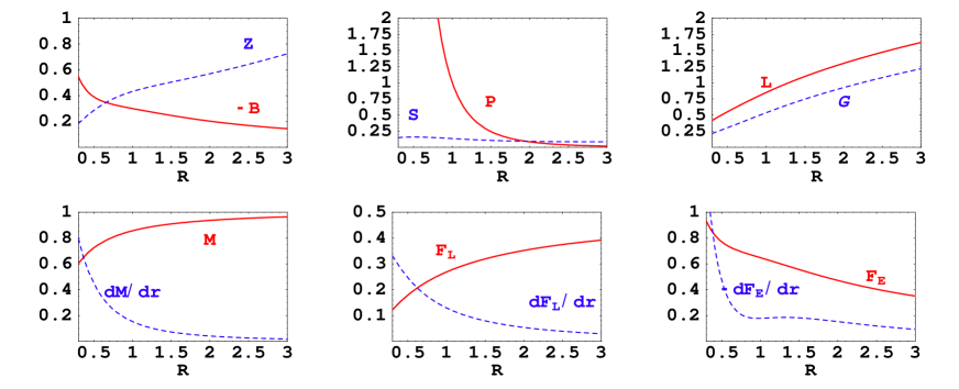
Figure 9: Model of the transition disk that connects the self-similar disk to an outer thin disk. The inner disk is chosen to have the parameters of fiducial Model I. The outer disk is a much thinner self-similar disk with $L(R)=0.95R^{1/2}$, $B(R)=-0.45R^{-1}$. The top three panels show the variation of the Bernoulli function $B$ and the disk thickness $Z=(P/{\cal P}\Omega^{2})^{1/2}$, the pressure $P$ and the entropy $S$, the angular momentum $L$ and the torque ${\cal G}$. The bottom three panels show the flows of mass, angular momentum and energy through the disk, and the associated outflows per unit radius.

These one-dimensional results can be used to verify that the disk remains stable according to the first Høiland criterion. If the disk remains gyrentropic, and the case for this weakens as it becomes increasingly radiative, then it is straightforward to repeat the analysis carried out in § 6.2 and construct a two-dimensional model. The gyrentropes remain close to right cylinders in the transition disk.

6.4 Choice of Disk–Outflow Model

We argued in § 2.1 that three internal parameters that characterise self-similar disks, which we chose to be $\ell_{0}$, $b_{0}$ and a torque parameter, determine the nature of the outflow, as measured by $n$, $\beta$ and $\eta$. How is this linkage established in practice? A comprehensive answer to this question must await more numerical experiments but some qualitative guidelines can be uncovered using our models. The first point is that angular momentum and mass are supplied to the adiabatic flow at the transition radius and are lost as the gas flows inward. Likewise, the energy derives from the relativistic regime and flows outward. The ratio of angular momentum flux to supplied mass flux in the transition region, $F_{L}/\dot{M}$, which is presumably set by local and outer boundary conditions, can have an influence on the subsequent inflow. If this ratio is large, then the disk will rotate rapidly and this can be propagated inward. Likewise, the energy per unit accreted mass — $F_{E}/\dot{M}$ — emerging from the relativistic inner disk controls the disk pressure and thickness and this can propagate outward.

However, this is not the whole story. The local physics within the self-similar regime is also important. If the rate of production of entropy near the disk surface is high, then mass loss will increase. Conversely, when it is low there will be more internal circulation to larger radii, where energy can escape more easily. If the disk has an organized magnetic field, then the loss of angular momentum per unit mass will be larger and the internal angular momentum transport will be diminished. Mathematically, we should think of coupled differential equations for the flows of mass, energy and angular momentum that have to be solved with boundary conditions at both small and large radius, just as with the theory of stellar structure.

7 Alternative Models of Adiabatic, Fluid Accretion

7.1 Non-Convective Models

In an alternative description of thick accretion disks, pioneered by Paczyński & Abramowicz (1982) for radiation-dominated tori, (cf. Rees et al. (1982) for the ion-dominated case), the flow is idealized as a quasi-stationary torus orbiting the black hole, in hydrostatic equilibrium with an ad hoc entropy distribution that is commonly chosen to be barytropic, $P=P(S)$. If this flow were convectively stable, the entropy would have to rise vertically as there can be no rotational stabilisation when a Høiland interchange is performed in the vertical direction. As there is a pressure maximum, and the isentropes coincide with the isobars in a barytropic flow, the isentropes would have to be a set of nested tori with minimum entropy at the pressure maximum.

However, this configuration cannot be stationary. To see this, note that the conservation laws, equations (52) and (56) (with $Q=0$), combine to give the entropy conservation law

$$\vec{G}\cdot\nabla\Omega+H\vec{J}\cdot\nabla\ln S=0.$$ (100)

Now, with a local torque, the first term in eq. (100) will be negative, consistent with the second law of thermodynamics (cf. Landau & Lifshitz (1959)). This implies that $\vec{J}\cdot\nabla\ln S>0$, i.e., there must be a mass flux directed toward increasing entropy. However, this would mean that there must be a mass source ($\nabla\cdot\vec{J}\neq 0$) at the pressure maximum. It is therefore clear that convectively stable, barytropic tori cannot be stationary. This conclusion is not altered by the inclusion of general relativity and is probably generally true for two-dimensional, Høiland-stable disk flows, although we have not been able to give a proof. Typically, what will happen is that any initially stable flow will quickly become convective, due to the action of the viscous stress, and the topology of the isentropes will change so that the entropy decreases with increasing cylindrical radius.

7.2 Advection-Dominated Accretion Flows

As outlined in § 1, the original ADAF idea (Ichimaru, 1977; Narayan & Yi, 1994, 1995) was that the inflow would be conservative with all the mass supplied at large radius flowing across the horizon. This would probably be the case as long as there were no angular momentum. However, as soon as the inflow is controlled by viscous torque that can be treated perturbatively, there seems no escape from the conclusion that most of the mass supplied escapes in an outflow, powered by the energy released by the small fraction of the gas that accretes onto the hole. (It is, in principle, possible that the viscous torques could be strong enough to ensure radial inflow which would vitiate this conclusion, but there is strong analytical and numerical evidence that neither fluid nor magnetofluid torques could ever be this large.) At a global level, the physical inconsistency is manifested in a positive Bernoulli function, indicating that parcels of matter near the surface of the disk can escape to infinity with positive energy after doing work on their surroundings. At a local level, the positive energy condition implies convective instability (in the hydrodynamic limit), providing a framework for understanding the mechanism of energy, angular momentum, and mass transport. In Paper II, we will show that analogous arguments carry over to magnetohydrodynamic disks, despite the fact that the stability and transport mechanisms are likely to be quite different.

For these reasons, we argue that black holes surrounded by radiatively inefficient flows are likely to accrete matter at a rate far smaller than the rate at which mass is supplied at large radii. The gas density close to the hole, from where most of the observed emission derives, is therefore likely to be orders of magnitude smaller than derived under the ADAF framework, implying that interpretations of observational data within the latter framework are incorrect. We note, however, that the ADIOS framework developed in this paper does not automatically predict the relationship between the accretion rate and the supply rate. This depends not only on additional information about the outer supply (or “transition”) radius, but also on the microphysical mechanisms that increase the entropy and power the wind at the thermal front. (In particular, the MHD winds to be discussed in Paper II may be capable of carrying away the required energy and angular momentum with very little loss of mass.)

7.3 Convection-Dominated Accretion Flows

The CDAF idea was developed to address the energetic difficulties encountered by ADAFs (Narayan, Igumenshchev & Abramowicz, 2000; Quataert & Gruzinov, 2000). These models are based on the surprising fact that fluid dynamical turbulence, as might arise, for example, from convection, is capable of transporting angular momentum radially inward in an accretion disk (cf.  Ryu & Goodman, 1992; Balbus, 2000; Quataert & Chiang, 2000). In CDAF models, it is supposed that the inward convective stress essentially balances the outward viscous stress locally. As a consequence, both the mass flux and the net angular momentum flux, which have different natural scalings with radius, must vanish while the energy flux is directed outward. In the two-dimensional model of Quataert & Gruzinov (2000), $B\sim 0$ everywhere and the flow must extend all the way to the pole. More detailed models assume that $B$ is very small, of order the binding energy at the outer (or transition) radius, and that a small conservative accretion flow is responsible for powering the outward flux of energy. The latter is assumed to be disposed of (e.g., by radiation or slow outflow) far from the black hole.

As convective transport is essentially nonlocal, there is no thermodynamic objection to the average convective torque being negative, although there may be thermodynamic limitations on the extent to which the (macroscopic) convective stress can cancel the (microscopic) viscous stress locally (Balbus & Hawley, 2002). However, the invocation of radial convective transport does seem arbitrary, given the nature of the convective instability. Recall that, at marginal stability in the hydrodynamic (non-MHD) limit, the unstable motions are along the gyrentropes, along roughly spherical surfaces. Radial modes are highly stable. Now if there is no means of extracting energy from the disk surface or the disk extends to the poles, then there will be no net transport and the disk may be forced toward a state in which radial convection can develop. This tendency may be present in numerical simulations by SPB99, some of which show large mass circulations with very small net mass flux.

Convection along gyrentropes is explicity suppressed, for example, in the CDAF model by Quataert & Gruzinov (2000), which extends all the way to the polar axis. We believe that this model is physically implausible for two reasons. The first is that flows that do not contain a central funnel have a singular velocity along the axis $v_{\phi}(0)=1$. The rates of shearing, dissipation and entropy production near the axis will therefore diverge, driving a powerful outflow which creates a funnel (cf. BB99). Because of the symmetry at this point, the viscous stress at the pole cannot be balanced by convective stresses. The second reason is that, unlike with the case of accretion onto a star, there is no means of supporting a column of gas along the rotation axis above a black hole: the centrifugal force acts along a perpendicular direction to the gravity and the pressure force must vanish close the event horizon of the hole (cf.  Narayan, Kato & Honma, 1997, , BB99). Once the funnel exists, we assert that convection will preferentially operate along gyrentropes, leading to mass and energy loss from the funnel walls.

CDAFs also face secular difficulties related to the global mass supply and energy flow. In CDAFs, as in ADIOS models, the accretion rate reaching the black hole is far smaller than the mass supply at large radii. However, unlike ADIOS models, there is no means of escape for the vast majority of the supplied matter, which does not make it to the black hole. In the hydrodynamical simulations by SPB99 and others, this is not an issue because these calculations track the evolution of a finite torus; matter is not continuously supplied. (Moreover, the runs are not long enough to track the evolution of the outer flow.) But in a CDAF with a continuous mass supply, there is no alternative but to establish an increasing reservoir of matter that is unable to accrete. Thus, CDAFs cannot represent steady-state flows. Moreover, there is a continuous flow of energy into the outer parts of a CDAF, where it will also build up unless there is some escape route. It has been proposed that the outer parts of ADAFs may adjust to radiate away this energy (Ball, Narayan & Quataert, 2001; Abramowicz & Igumenshchev, 2001), but it has not been demonstrated that this will happen naturally. Another possibility is that the energy flux will power a wind at some outer radius. We contend that this too is a less likely resolution than a scheme in which the wind is released continously from all radii.

Even if CDAFs did not face these severe physical problems, their existence seems unlikely to carry over to the MHD case, which is more appropriate to astrophysical disks than the hydrodynamical limit. The dominant instabilities in magnetized disks are magnetorotational, rather than convective, and the resulting turbulence is likely to transport angular momentum outward rather than inward (Balbus & Hawley, 2002); but see Narayan et al. (2002); Igumenshchev (2002) for an alternative view. If this is the case, then the CDAF approach cannot be generalized to MHD flows. However, we will argue in Paper II that the ADIOS approach does carry over. Although MHD disks cannot attain marginal stability, they nevertheless appear to develop a well-defined internal structure (barytropicity, with rotation on cylinders), that provides an equivalent autonomous constraint to our hydrodynamical assumption of gyrentropicity. Thus, MHD disks admit well-defined circulation patterns and outflows, which we will derive explicitly in Paper II.

7.4 Weakly-Bound Disks

Finally, we comment on a class of non-radiative accretion models most recently studied by Paczyński (1998), but which enjoyed wide popularity in the early 1980’s (e.g.,  Jaroszyński, Abramowicz & Paczyński, 1980; Paczyński & Wiita, 1980, and references therein). In these models the angular momentum distribution is prescribed, usually as a function of cylindrical radius along the surface of the flow, between some inner radius $r_{\rm in}$ and some outer radius $r_{\rm out}$. At $r\geq r_{\rm out}$ the flow is assumed to match a thin Keplerian accretion disk, while at $r\rightarrow r_{\rm in}$ the flow approaches a zero-pressure cusp through which material accretes onto the black hole. For the interesting limit of $r_{\rm out}\gg r_{\rm in}$ the gas in the advection-dominated region is very weakly bound and one can show (Paczyński, 1998) that the cusp must lie close to the marginally bound orbit at $r=4m$ (for a Schwarzschild black hole). There is considerable latitude in the choice of angular momentum distribution, subject to the constraints that the angular momentum must be a monotonically increasing function of $r$, and that the angular momentum and binding energy must match the Keplerian values at both $r_{\rm in}$ and $r_{\rm out}$.

One of the rationales for exploring these models is that the generic form of the angular momentum distribution is physically motivated, whereas viscous stress prescriptions are highly uncertain. It is therefore worthwhile, Paczyński argues, to construct a model based on an assumed angular momentum law, and then see what kind of viscous stress prescription is required to make it self-consistent. However, in his published work he does not discuss the nature of these stress prescriptions. We now show that weakly bound disk models require very specific and (we believe) implausible prescriptions for the viscous stress.

We restrict our attention to the limit $r_{\rm out}\gg r_{\rm in}$ and use the notation in Paczyński (1998). Paczyński (1998) eq. (25) implies that the binding energy is a monotonically increasing function of $r_{s}$, the cylindrical radius measured along the surface. This implies the inequality

$$\int^{r_{s}}_{r_{\rm in}}{1\over r^{2}}{dj_{s}^{2}\over dr}dr<{2j_{\rm out}^{2}\over r_{\rm out}^{2}}\approx{1\over 2r_{\rm out}r_{\rm in}}j_{\rm in}^{2}$$ (101)

for all $r_{\rm in}<r_{s}<r_{\rm out}$. Integrating by parts, and using the inequality $j_{s}\geq j_{\rm in}$, we finally obtain

$$j_{s}^{2}<j_{\rm in}^{2}\left(1+{r_{s}^{2}\over 2r_{\rm out}r_{\rm in}}\right).$$ (102)

Thus, the angular momentum distribution must be a very weak function of radius, $j\approx j_{\rm in}$ for $r_{s}$ smaller than the geometric mean between $r_{\rm in}$ and $r_{\rm out}$. In other words, any acceptable angular momentum distribution for this kind of model must be nearly constant in the inner part of the disk, while increasing more steeply than Keplerian in the outer parts (in order to satisfy the outer boundary condition).

Inequality (102) places severe constraints on the viscous stress. Using the $\alpha$-model viscous couple assumed by Afshordi & Paczyński (2002) which differs from our assumed torque (eq. [49]) by a factor $\Omega/\Omega_{\rm Kep}$, and assuming an internal sound speed $v_{s}\sim v_{\rm Kep}$ (appropriate for a thick disk), we obtain an inflow speed $v_{r}$ given by

$${-v_{r}\over v_{\rm Kep}}\approx\alpha{j_{s}\over j_{s}-j_{\rm in}}\left(-{d\ln\Omega\over d\ln r}\right).$$ (103)

Substituting from inequality (102) in the limit $r_{s}\ll(r_{\rm in}r_{\rm out})^{1/2}$, we can write eq. (103) in the form

$$\alpha<{r_{s}^{2}\over 8r_{\rm in}r_{\rm out}}{-v_{r}\over v_{\rm Kep}}.$$ (104)

The hydrostatic condition implies $-v_{r}/v_{\rm Kep}\ll 1$, placing a tight upper limit on $\alpha$. The limit is even more severe if we use our expression (49) for the stress.

If $\alpha$ exceeds the limit given in eq. (104), over any range of radii, then the inflow will proceed on a free-fall timescale, violating a principal assumption of the model. This will presumably continue until the angular momentum distribution relaxes to state closer to Keplerian, in which case it will resemble one of the models discussed above (i.e., an ADAF, CDAF, or ADIOS). It will also evolve toward a larger binding energy. We would, of course, argue that the only self-consistent final state under these circumstances would be an ADIOS.

Physically, we expect the value of $\alpha$, or its equivalent in a more realistic stress model, to be set by the microphysics of the accretion process and not by the global boundary conditions — the latter presumably reflect the cooling function of the gas and/or the nature of the gas supply at $r_{\rm out}$. Numerical models of MHD flows suggest that $\alpha$ may fall in the range $\sim 0.01-0.1$, which is inconsistent with the limit derived above unless $r_{\rm out}\la 100r_{\rm in}$. Observations of adiabatic accretion flows suggest that $r_{\rm out}$ may be larger than $\sim 10^{4}-10^{5}$ times $r_{\rm in}$. Such systems would have to have an effective $\alpha<10^{-5}$ in order to be described self-consistently by a Paczyński model. Thus, we conclude that weakly bound disk models are unlikely to apply in many, if not most, cases of astrophysical interest.

8 Discussion

We have attempted to flesh out the ADIOS concept by constructing explicit, two-dimensional models of adiabatic, accreting fluid. Such flows are strongly convective and should naturally evolve toward a state of marginal stability. We argue that the convective transport of energy and angular momentum does not occur primarily in the radial direction but, instead, proceeds primarily along surfaces that connect the equatorial region to the disk “surface” at high latitudes. We have demonstrated how to construct models of two-dimensional disks embodying these principles, and have then elaborated upon them so as to include poloidal circulation, inflow and the formation of fluid outflows.

Even in the context of purely fluid disks, our approximate description of the flow can be challenged. For example, if the viscous stress, as measured by the parameter $\alpha$, is not small, the perturbative ordering: circular speed $\gg$ convective speed $\gg$ meridional circulation/inflow speed will not be well-satisfied as we require. Our thermal front model for producing the outflow is, likewise, an oversimplification. It posits a site where entropy is produced and simple conservation laws make explicit the connection between the energy flow along the gyrentropes and the outflow. It seems reasonable that the dissipation should be a strongly increasing function of the Mach number and that it be efficient when the flow becomes roughly sonic but this is not required. If the surface dissipation is small, we suppose that the energy will be advected by the circulation to large radius. Indeed, as discussed in § 3.2, several simulations do seem to show this behaviour which is not consistent with a self-similar flow. Higher resolution simulations that are run for long enough to achieve a stationary flow will be needed to understand the flow of mass, angular momentum and energy through the disk.

Another concern is that our calculation is expressly two-dimensional and it is well-known that three-dimensional convection in non-rotating fluid is quite different from its two-dimensional counterpart. However, if our convection model is realistic, it automatically leads to considerable smoothing over azimuth which ought to validate the two-dimensional description. A related concern involves the unstable, non-axisymmetric, global instabilities that can develop in the relativistic inner disk described in § 6.2 (Papaloizou & Pringle, 1984). As these modes rely upon reflection from the inner surface of the disk, they are unlikely to grow to a large amplitude in the presence of inflow (Begelman, Blandford & Rees, 1984; Blaes, 1987).

The most fundamental limitation concerns the explicit neglect of magnetic field in our model. Beyond all reasonable doubt, the torque in astrophysical accretion disks is hydromagnetic in origin (Balbus & Hawley, 1998). If the magnetic fields remained small in strength and length scale and were locally dissipative, then our treatment could still have validity. However, the evidence from numerical simulations is that none of these conditions is well-satisfied in practice. In particular, the relationship between the momentum transfer and the dissipation is problematic. With a simple, Newtonian viscosity, the connection is clear. There is a local dissipation at a rate $\vec{G}\cdot\nabla\Omega$. Entropy is created where the torque is applied. The introduction of convection into fluid models complicates this linkage, because it involves the net bodily transfer of mass carrying its own angular momentum and energy and transporting an additional energy flux. This effectively makes the dissipation nonlocal. As we shall discuss in Paper II, magnetized disks may provide even more extreme examples of non-local dissipation. Unless a magnetic turbulence spectrum is established and the energy cascades down to a small inner scale where it can be taken up by plasma, much of the dissipation may be non-local. Indeed, there is plenty of evidence that much of the dissipation in observed disks occurs in a hot corona. (In considering this problem it is important to make the distinction between ion-supported and radiation-supported disks. The former require that local dissipation not heat the electrons to temperatures where they can radiate efficiently, implying either that most of the energy either goes into heating the ions or that the energy is transported away. By contrast, radiation-dominated accretion disks are subject to the magnetorotational instability but the magnetic stress may saturate at a lower level, perhaps validating a treatment closer to our fluid models.)

The final missing ingredient is an allowance for global time-dependence in the flow. There are strong indications that observed disks accrete episodically. Whether or not this happens in practice, on all radial scales, depends upon the details of the transition region. In § 6.3, we argue that there could be a smooth, stationary transition from a radiative thin disk to an ADIOS. However, if the outflow is less efficient than we have assumed in carrying off the energy, circulation of the excess energy to the transition region will push it outward to progressively larger radii until there is catastrophic cooling so that the thick disk quickly shrinks. The whole pattern can repeat in a limit cycle. However, as the inflow and dynamical timescales are always likely to increase with radius, these variations should only cause a slow secular change in the flow pattern at small radii, where most of the accretion energy is released. In the language of our models this would be manifested in a change in the entropy scale $s_{0}$ (cf. § 4.3). The other way in which time-dependence could be important is if there are local instabilities in the flow pattern. In the case of adiabatic accretion disks the distinction between viscous and thermal timescales is blurred. This, coupled with the physical thickness of the disk, makes a formal instability calculation more complicated and we advocate direct numerical simulation as the means to explore stability of these flows. Few simulations have been evolved long enough to draw strong conclusions about time-dependence.

We believe that the fluid dynamical analysis is valuable because it suggests a “modular” procedure for analysing numerical simulations of magnetized flows:

1. Determine the rule that replaces gyrentropicity for determining the time-averaged disk structure. We will argue in Paper II, on the basis of numerical simulations and analytic calculations, that this principle may be barytropicity, implying rotation on cylinders.

2. Separate the motion into relatively small scale interchanges – with scales no larger than the local pressure scale height, and larger circulatory flows. The former can be analysed by computing correlation functions involving velocity, pressure, density, etc., up to third order so as to understand the time-averaged transport of mass, angular momentum and energy as a function of position. The latter will describe the global flow pattern.

3. Understand the surface boundary condition, specifically the strength and character of the MHD wind from the disk surface. Central to answering this question is to decide whether or not large scale magnetic fields are generated, as is observed in the high latitude wind from the quiet sun, or whether the fields are tangled on small scale and behave as an anisotropic gas. This problem will be very hard to tackle as it combines both local and global features.

We shall address these issues further in Paper II.

Despite all of these shortcomings and concerns, we hope that the models developed in this paper will provide a guide to interpreting numerical simulations and, ultimately, the increasingly detailed observations of radiation from adiabatically accreting black holes and neutron stars.

References

- Abramowicz et al. (1995) Abramowicz M. A., Chen X., Kato S., Lasota J. P., Regev, O., 1995, ApJ, 438, L37
- Abramowicz & Igumenshchev (2001) Abramowicz M. A., Igumenshchev, I. V., 2001, ApJ, 554, L53
- Abramowicz, Lasota & Igumenshchev (2000) Abramowicz M. A., Lasota J.-P., Igumenshchev I., 2000, MNRAS, 314, 775
- Afshordi & Paczyński (2002) Afshordi N., Paczyński B., 2002, astro-ph/0202409
- Agol (2000) Agol E., 2000, ApJ, 538, L121
- Aitken et al. (2000) Aitken D. K. et al., ApJ, 530, 173
- Allen et al. (2000) Allen S. W., Di Matteo T., Fabian A. C., 2000, MNRAS, 311, 493
- Baganoff et al. (2001) Baganoff F. K. et al., 2001, ApJ, submitted, astro-ph/0102151
- Balbus (2000) Balbus S. A., 2000, ApJ, 534, 420
- Balbus & Hawley (1998) Balbus S. A., Hawley J. F., 1998, RMP, 70, 1
- Balbus & Hawley (2002) Balbus S. A., Hawley J. F., 2002, ApJ, 573, 749
- Ball, Narayan & Quataert (2001) Ball G. H., Narayan R., Quataert E., 2001, ApJ, 552, 221
- Bardeen (1973) Bardeen J. M., 1973, in DeWitt C., DeWitt B., eds., Black Holes. Gordon & Breach, New York.
- Bardeen & Berger (1978) Bardeen J. M., Berger B. K., 1978, ApJ, 221, 105
- Begelman (1979) Begelman M. C., 1979, MNRAS, 187, 237
- Begelman (2002) Begelman M. C., 2002, ApJ, 568, 97
- Begelman, Blandford & Rees (1984) Begelman, M. C., Blandford, R. D. & Rees, M. J., 1984, Rev. Mod. Phys., 56, 255
- Begelman & Meier (1982) Begelman M. C., Meier D. L., 1982, ApJ, 253, 873
- Blaes (1987) Blaes, O. M., 1987, MNRAS, 227, 975
- Blandford (1984) Blandford R. D., 1984, in Evans D. S., ed., Eleventh Texas Symp. on Relativistic Astrophysics. Ann. NY Acad. Sci., 422, p. 303
- Blandford & Begelman (1999) Blandford R. D., Begelman M. C., 1999, MNRAS, 303, L1 (BB99)
- Blandford, Jaroszyński & Kumar (1985) Blandford R. D., Jaroszyński M., Kumar S., 1985, MNRAS, 215, 667
- Blandford & Payne (1982) Blandford R. D., Payne D. G., 1982, MNRAS, 199, 883
- Bower et al. (2003) Bower G. C., Wright M. C., Falcke H., Backer D. C., 2003, ApJ, 588, 331
- Di Matteo et al. (1999) Di Matteo T., Fabian A. C., Rees M. J., Carilli C. L., Ivison R. J., 1999, MNRAS, 305, 492
- Di Matteo et al. (2000) Di Matteo T., Quataert E., Allen S. W., Narayan R., Fabian A. C., 2000, MNRAS, 311, 507
- Fabian (2003) Fabian A. C., 2003, in Ho L., ed., Carnegie Observatories Astrophysics Series, Vol. 1: Coevolution of Black Holes and Galaxies. Cambridge Univ. Press, Cambridge, in press. astro-ph/0304122
- Frank, King & Raine (2001) Frank J., King A. R., Raine D. J., 2001, Accretion Power in Astrophysics. Cambridge Univ. Press, Cambridge
- Galeev et al. (1979) Galeev A. A., Rosner R., Vaiana G. S., 1979, ApJ, 229, 318
- Goldreich & Schubert (1967) Goldreich P., Schubert G., 1967, ApJ, 150, 571
- Hansen & Kawaler (1994) Hansen C. J., Kawaler S. D., 1994, Stellar Interiors: Physical Principles, Structure, and Evolution. Springer, Berlin
- Ichimaru (1977) Ichimaru S., 1977, ApJ, 214, 840
- Igumenshchev (2002) Igumenshchev I. V., 2002, ApJ, 577, 31
- Jaroszyński, Abramowicz & Paczyński (1980) Jaroszyński M., Abramowicz M. A., Paczyński B., 1980, Acta Astr., 30, 1
- Kato & Nakamura (1998) Kato S., Nakamura K. E., 1998, PASJ, 50, 559
- King, Taam & Begelman (2000) King A. R., Taam R., Begelman M. C., 2000, ApJ, 530, L25
- Königl & Pudritz (2000) Königl A., Pudritz R. E., 2000, in Mannings V., Boss A. P., Russell S. S., eds., Protostars and Planets IV, p. 759. Univ. of Arizona Press, Tucson
- Landau & Lifshitz (1959) Landau L. D., Lifshitz E. M., 1959, Fluid Mechanics. Pergamon, Oxford
- Manmoto et al. (2000) Manmoto T., Kato S., Nakamura K. E., Narayan R., 2000, ApJ, 529, 127
- Margon (1984) Margon, B. 1984, ARA&A, 22, 507
- Melia & Falcke (2001) Melia F., Falcke H., 2001, ARA&A, 39, 309
- Mirabel & Rodriguez (1999) Mirabel, I. F., Rodriguez, L. F., 1999, ARA&A, 37, 409
- Mushotzky et al. (2000) Mushotzky R., Angelini L., Arnaud K. A., Loewenstein M., 2000, AAS High Energy Astrophysics Division, 32, 2101
- Narayan & Yi (1994) Narayan R., Yi I., 1994, ApJ, 428, L13
- Narayan & Yi (1995) Narayan R., Yi I., 1995, ApJ, 444, 231
- Narayan, Kato & Honma (1997) Narayan R., Kato S., Honma F., 1997, ApJ, 476, 49
- Narayan, Igumenshchev & Abramowicz (2000) Narayan R., Igumenshchev I. V., Abramowicz M. A., 2000, ApJ, 539, 798
- Narayan, Mahadevan & Quataert (1999) Narayan R., Mahadevan R., Quataert E., 1998, in Abramowicz M. A., Bjornsson G., Pringle J. E., eds., The Theory of Black Hole Accretion Disks, p. 148. Cambridge Univ. Press, Cambridge
- Narayan et al. (2002) Narayan R., Quataert E., Igumenshchev I. V., Abramowicz M. A., 2002, ApJ, 577, 295
- Paczyński (1998) Paczyński B., 1998, Acta Astr., 48, 667
- Paczyński & Abramowicz (1982) Paczyński B., Abramowicz M. A., 1982, ApJ, 253, 897
- Paczyński & Wiita (1980) Paczyński B., Wiita P., 1980, A&A, 88, 23
- Papaloizou & Pringle (1984) Papaloizou, J. C. B. & Pringle, J. E., 1984, MNRAS, 208, 721
- Quataert & Chiang (2000) Quataert E., Chiang E. I., 2000, ApJ, 543, 432
- Quataert & Gruzinov (2000) Quataert E., Gruzinov A., 2000, ApJ, 539, 809
- Quataert & Narayan (1999) Quataert E., Narayan R., 1999, ApJ, 520, 298
- Rees et al. (1982) Rees M. J., Begelman M. C., Blandford R. D., Phinney E. S., 1982, Nature, 295, 17
- Ryu & Goodman (1992) Ryu D., Goodman J., 1992, ApJ, 388, 438
- Seguin (1975) Seguin F., 1975, ApJ, 197, 745
- Shakura & Sunyaev (1973) Shakura N. I., Sunyaev R. A., 1973, A&A, 24, 337
- Sołtan (1982) Sołtan A., 1982, MNRAS, 200, 115
- Stone & Pringle (2001) Stone J. M., Pringle J. E., 2001, MNRAS, 322, 461
- Stone, Pringle & Begelman (1999) Stone J. M., Pringle J. E., Begelman M. C., 1999, MNRAS, 310, 1002 (SPB99)
- Tassoul (1978) Tassoul J.-L., 1978, Theory of Rotating Stars. Princeton Univ. Press, Princeton
- Weymann (1997) Weymann R., 1980, in Arav N., Shlosman I., Weymann R. J., eds., Mass Ejection from AGN, p. 3. Astron. Soc. Pacific, San Francisco
- Yu & Tremaine (2002) Yu Q., Tremaine S. D., 2002, MNRAS, 335, 965