Galactic cannibalism in the galaxy cluster C0337-2522 at ${\bf z=0.59}$

Abstract

According to the galactic cannibalism model, cD galaxies are formed in the center of galaxy clusters by merging of massive galaxies and accretion of smaller stellar systems: however, observational examples of the initial phases of this process are lacking. We have identified a strong candidate for this early stage of cD galaxy formation: a group of five elliptical galaxies in the core of the X-ray cluster C0337-2522 at redshift $z=0.59$. With the aid of numerical simulations, in which the galaxies are represented by N-body systems, we study their dynamical evolution up to $z=0$; the cluster dark matter distribution is also described as a N-body system. We explore the hypothesis that some of the five galaxies will have merged before $z=0$, making reasonable assumptions on the structural and dynamical characteristics of the cluster. We then compare the properties of the merger remnant with those of real ellipticals (such as its accordance with the Fundamental Plane, the Faber-Jackson, and the $M_{\rm BH}$-$\sigma_{0}$ relations) and, in particular, we check whether the remnant has the surface brightness profile typical of cD galaxies. We find that a multiple merging event in the considered group of galaxies will take place before $z=0$ and that the merger remnant preserves the Fundamental Plane and the Faber–Jackson relations, while its behavior with respect to the $M_{\rm BH}$-$\sigma_{0}$ relation is quite sensitive to the details of black hole merging. However, the end–products of our simulations are more similar to a “normal” giant elliptical than to a cD galaxy with its characteristic diffuse luminous halo, thus confirming previous indications that the formation of cD galaxies is not a necessary consequence of galaxy merging at the cluster center.

1 Introduction

Among the various scenarios proposed for the formation of the brightest cluster galaxies (BCGs), and in particular of cD galaxies, perhaps the most prominent is the so–called “galactic cannibalism” model (Ostriker & Tremaine 1975, Hausman & Ostriker 1978). In this picture super-luminous ellipticals (hereafter Es) are formed in the center of galaxy clusters by merging of massive galaxies and by accretion of smaller stellar systems. Indeed, numerical simulations have shown that galactic cannibalism is able to reproduce many properties of the observed BCGs (see, e.g., Miller 1983, Merritt 1984, Malumuth & Richstone 1984, Bode et al. 1994, Athanassoula, Garijo & Garcia Gomez 2001). However, there are still some significant discrepancies between the predictions of these simulations and the observations: in particular, if one considers the available numerical simulations it is apparent that only a small fraction of the simulations ending in a merging event do produce a cD-like galaxy, while observations reveal that the presence of a cD galaxy is quite a common property of galaxy clusters (see, e.g., Dressler 1984, and references therein). In addition, Thuan & Romanishin (1981) pointed out that BCGs in poor clusters do not show the diffuse luminous envelope typical of cDs, and this could be an important additional indication that the end–product of galactic cannibalism not necessarily consists in a cD galaxy.

Observational tracers of the late stages of cD galaxy formation have already been found: for example, the high frequency of multiple nuclei in cD galaxies is considered an indication of recent merging (see, e.g., Matthews, Morgan & Schmidt 1964, Schneider, Gunn & Hoessel 1983, Laine et al. 2003). On the contrary, observational examples of the initial stages of cD galaxy formation are lacking: according to the scenario depicted above, such systems would appear as groups of galaxies located in the core of clusters and spiraling, as an effect of dynamical friction, towards the cluster center. We have identified a strong candidate for such an evolutionary stage: a group of five Es located within a region of a few kpc of (projected) linear size near the center of the X-ray selected cluster C0337-2522 at redshift $z=0.59$ (ROSAT Deep Cluster Survey; Rosati et al. 1998).

The main goal of this work is to explore, as a function of the initial conditions and of the structural and dynamical characteristics of their parent cluster, how many (if any) of the five galaxies under consideration will have merged before $z=0$. In addition, we investigate whether the remnant has the surface brightness (SB) profile typical of cD galaxies, i.e., it possesses a diffuse low luminosity halo. Finally, we check whether some features of Es, such as the Fundamental Plane (FP; Djorgovski & Davis 1987; Dressler et al. 1987), the Faber-Jackson relation (FJ; Faber & Jackson 1976), the $M_{\rm BH}$-$\sigma_{0}$ relation (Gebhardt et al. 2000; Ferrarese & Merritt 2000) and the metallicity gradient (Peletier 1989, Carollo, Danziger & Buson 1993), are preserved during the process. This kind of investigation is motivated by the fact that BCGs, both giant Es and cDs, follow quite closely the FP and the FJ relation determined by less luminous Es (see, e.g., Oegerle & Hoessel 1991), though there are indications that a significant fraction of BCGs are brighter than would be expected from the FJ relation of normal Es (Malumuth & Kirshner 1981, 1985). BCGs have also metallicity gradients consistent with those of normal Es (Fisher, Franx & Illingworth 1995), and those for which the mass of the central supermassive black hole (BH) has been measured do follow the $M_{\rm BH}$-$\sigma_{0}$ relation (e.g., M87; Gebhardt et al. 2000, Ferrarese & Merritt 2000).

We try to address the questions above with the aid of numerical simulations in which the galaxies are represented by N-body systems, and the initial conditions are constrained by the imaging and kinematic information from our ESO-VLT data. The observations provide, for each galaxy, only three phase–space coordinates (the two projected positions and the line–of–sight velocity); thus, some assumptions are needed in order to assign the remaining initial conditions. In principle, one could make use of non-parametric estimators (see Merritt & Trembley 1994); however, given the small number of objects involved, such estimators are not practical for our application. To overcome this problem, we modeled the cluster where the five galaxies reside as a spherical dark matter (DM) density distribution with adjustable total mass, scale length and amount of radial orbital anisotropy in the velocity distribution: in order to explore the effects of the dynamical friction of the galaxies against the cluster DM, also the cluster is represented as a live N-body system.

This paper is organized as follows. The observations and the galaxy models are presented in Section 2 and Section 3, respectively. A description of the simulations is given in Section 4 and the results are discussed in Section 5. Our conclusions are presented in Section 6.

2 Observations and data reduction

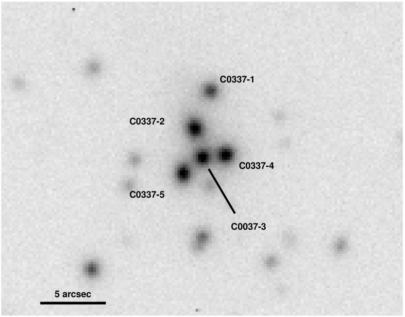
Figure 1: VLT-FORS1 I-band image of the galaxy cluster C0337-2522 (N up, E left). The five galaxies are named as in Table 1.

The five galaxies that we have considered are located in the core of the X-ray galaxy cluster C0337-2522. The I-band image, shown in Fig. 1, was obtained in September 1999, using the Focal Reducer and Spectrograph 1 (FORS1) at the ESO Very Large Telescope (VLT) with exposure time $2\times 300$s and seeing $0.9^{\prime\prime}$. The image was reduced with standard procedure and a catalogue of the objects was carried out with the SExtractor package (Bertin & Arnouts 1996). Spectra for the five elliptical galaxies were obtained in January 2000 with FORS1 at VLT, using the grism R600 and a $1^{\prime\prime}$ wide slit with a resolution of $\approx 90\,-\,100\,{\rm km\,s^{-1}}$; exposure times were in the range $2700\,-\,7200\,{\rm s}$. The reduction of the spectroscopic data and the measurement of the redshifts (reported in Table 1) were performed following the procedures described in Treu et al. (2001). We note that, due to poor weather conditions and reduced reflectivity during the early-stages of operations (see, e.g., Labbé et al. 2003), the S/N ratio of the spectroscopic data does not allow us to measure with sufficient accuracy the central velocity dispersions for all the five galaxies. Thus, in the present work we are unable to use velocity dispersion measurements in order to constrain the total mass of the galaxies and their internal dynamics. The details of the photometric measurements will be presented in a separate paper (Treu et al. 2003). For the aim of this paper it suffices to say that the five galaxies have very similar (within $\sim 0.5$ mag, see Table 1) I-band magnitudes, typical of bright cluster E/S0 at that redshift (see, e.g., Kelson et al. 1997). We have no information about other low–luminosity members of the cluster, and so we decided to consider only the five galaxies in the simulations, except for a special simulation described in Section 6. Note also that some doubt about the cluster membership of galaxy C0337-2 could be reasonably raised by considering its negative and high barycentric velocity: however, the cluster X-ray emission (Rosati et al. 1998; see also Vikhlinin et al. 1998) strongly points towards the physical association of the central group of galaxies. We decided to consider also galaxy C0337-2 as a member of the cluster: its “special” dynamical status will be however evident when discussing the results of the simulations.

Table 1: Known data for the five galaxies. Positions and velocities are relative to the center of mass of the system. For reference, the center of galaxy C0337-4 is at $\alpha=03{\rm h}37{\rm m}45.15{\rm s}$ and $\delta=-25^{o}22^{\prime}36\aas@@fstack{\prime\prime}1$ (J2000). I-band aperture photometry within a $1^{\prime\prime}$ diameter aperture together with its random uncertainty is listed in the last column (the zero point of the magnitude scale is accurate to 0.1 mags).

Galaxy	redshift	$x$	$y$	$v_{z}$	$x$	$y$	I
		(arcsec)	(arcsec)	(km/s)	(kpc)	(kpc)	(mag)
C0337-1	0.589	0.51	3.78	284.7	3.63	27.00	20.55 $\pm$ 0.05
C0337-2	0.578	-0.36	0.94	-1892.9	-4.51	6.71	20.02 $\pm$ 0.06
C0337-3	0.590	-0.01	-1.24	473.3	-0.09	-8.86	19.98 $\pm$ 0.12
C0337-4	0.592	1.63	-1.04	850.2	11.63	-7.43	20.03 $\pm$ 0.05
C0337-5	0.589	-1.49	-2.44	284.7	-10.66	-17.43	20.11 $\pm$ 0.05

3 Models

The initial conditions for the cluster and the galaxies are spherically symmetric density distributions. In particular, for the cluster DM distribution we use a Hernquist (1990) model: note that in the central regions it is indistinguishable from the Navarro, Frenk & White (1996) density profile, while characterized by finite total mass. Thus,

$$\rho_{\rm cl}(r)={M_{\rm cl,tot}r_{\rm cl}\over 2\pi r(r_{\rm cl}+r)^{3}},$$ (1)

$${M_{\rm cl}(r)\over M_{\rm cl,tot}}=\left({r\over r_{\rm cl}+r}\right)^{2},$$ (2)

$${\Psi_{\rm cl}(r)}={GM_{\rm cl,tot}\over r_{\rm cl}+r},$$ (3)

where $\rho_{\rm cl}(r)$ is the cluster density profile, $M_{\rm cl}(r)$ and $M_{\rm cl,tot}$ are the mass within the radius $r$ and the total cluster mass, respectively, $\Psi_{\rm cl}(r)$ is the relative (positive) potential, and $r_{\rm cl}$ is the so–called “core radius”. For the galaxies we use both one and two–component Hernquist models (Ciotti 1996), and so the galaxy stellar and DM components are also described by equations (1)-(3), where the subscripts “*” and “h” now identify the two distributions, respectively. In the two–component models we always assume $M_{\rm h,tot}\equiv 5M_{\rm*,tot}$ and $r_{\rm h}\equiv 3r_{\rm*}$.

We note that a certain amount of radial orbital anisotropy is expected in some of the current structure formation scenarios of Es (see, e.g., van Albada 1982, Barnes 1992, Hernquist 1993) and clusters (see, e.g., Crone, Evrard & Richstone 1994, Cole & Lacey 1996, Ghigna et al. 1998). However, there exist observational and theoretical indications that the amount of radial anisotropy should be modest in the both cases (see, e.g., Carollo et al. 1995, Ciotti & Lanzoni 1997, van der Marel et al. 2000, Gerhard et al. 2001, Nipoti, Londrillo & Ciotti 2002, hereafter NLC02), even at significant look-back times (Koopmans & Treu 2003). Accordingly, in a subset of simulations, the cluster and/or the galaxy stellar components are radially anisotropic, while for sake of simplicity the galactic DM halo component is always isotropic. In practice, radial orbital anisotropy is introduced by using the Osipkov-Merritt parameterization (Osipkov 1979; Merritt 1985), where the supporting distribution function (DF) for the density profile $\rho$ is given by

$$f(Q)=\frac{1}{\sqrt{8}\pi^{2}}\frac{d}{dQ}\int_{0}^{Q}{\frac{d{\varrho}}{d\Psi_{\rm T}}}{\frac{d\Psi_{\rm T}}{\sqrt{Q-\Psi_{\rm T}}}},$$ (4)

with

$$\varrho(r)=\left(1+\frac{r^{2}}{r_{\rm a}^{2}}\right)\rho(r),$$ (5)

and $f(Q)=0$ for $Q\leq 0$. The quantity $Q$ is defined as $Q\equiv{\mathcal{E}}-{L^{2}/2r_{\rm a}^{2}}$, where ${\mathcal{E}}=\Psi_{\rm T}-v^{2}/2$ is the relative (positive) energy per unit mass, $v$ is the modulus of the velocity vector, $\Psi_{\rm T}$ is the relative total gravitational potential, and $L$ is the modulus of the angular momentum per unit mass. The parameter $r_{\rm a}$ is the so–called “anisotropy radius”. For $r\gg r_{\rm a}$ the velocity dispersion tensor is radially anisotropic, while for $r\ll r_{\rm a}$ it is nearly isotropic. The isotropic DF is given by equation (4) in the limit $r_{\rm a}\to\infty$. Following the adopted notation, we indicate the anisotropy radius of the cluster and of the galaxies as $r_{\rm a,cl}$ and $r_{\rm a,*}$, respectively.

4 Numerical simulations

4.1 Initial conditions

The coordinate system adopted to describe Fig. 1 is defined so that the $x$-axis runs east–west, the $y$-axis runs south–north, and the $z$-axis is along the line–of–sight. Observations provide only 3 of the required 6 initial phase–space coordinates of the center of mass of each galaxy, namely two positions in the $(x,y)$ projected plane and the line–of–sight velocity $v_{z}$. The problem of the orbital evolution of the five galaxies is thus underdetermined, and the missing initial coordinates force us towards a probabilistic approach, where several initial conditions compatible with the observational constraints are used to evolve the system from $z=0.59$ to the present. We assume, for simplicity, that the five galaxies have equal masses (see Section 2), and that in the inertial reference system centered on the cluster center $\sum{x_{i}}=\sum{y_{i}}=\sum{z_{i}}=\sum{v_{x,i}}=\sum{v_{y,i}}=\sum{v_{z,i}}=0$, summing over the five galaxies. In Table 1 we report the values of the known coordinates for the five galaxies, reduced to the reference system (we adopted $\Omega_{\rm m}=0.3$, $\Omega_{\rm\Lambda}=0.7$, and $H_{0}=65$ km s^-1 Mpc^-1).

In order to fix the missing coordinates $(z_{i},v_{x,i},v_{y,i})$ of the galaxies, as a first step we constrain the structural and dynamical properties of the cluster model, by choosing the values of the parameters $s_{\rm a,cl}$, $r_{\rm cl}$, and $M_{\rm cl,tot}$ (see Section 3). We investigated two cases for the DF of the cluster: the isotropic case (corresponding to $s_{\rm a,cl}\equiv r_{\rm a,cl}/r_{\rm cl}=\infty$) and the radially anisotropic case with $s_{\rm a,cl}=1.8$, a value that fiducially corresponds to the maximum degree of radial anisotropy compatible with stability for the one–component Hernquist model (see, e.g., NLC02, and references therein). For $r_{\rm cl}$, we adopted the values $100$ kpc and $300$ kpc (corresponding to half-mass radius $r_{\rm M,cl}\simeq 241$ kpc and $r_{\rm M,cl}\simeq 724$ kpc, respectively): note that, at least in projection, all the five galaxies are well within $r_{\rm cl}$. Obviously, for a fixed $r_{\rm cl}$ there is a minimum cluster mass ($M_{\rm min}$) for which all the five galaxies are bound, under the implicit assumption that the cluster DM is virialized (consistently with the time independence of the cluster potential). For each galaxy, the lower limit to the cluster mass corresponds to the case of vanishing $v_{x}$, $v_{y}$ and $z$: then $M_{\rm min}$ is given by the maximum of these 5 lower limits. From the values in Table 1 and from equation (3), $M_{\rm min}\simeq 4.4\times 10^{13}M_{\odot}$, when $r_{\rm cl}=100$ kpc, and $M_{\rm min}\simeq 1.28\times 10^{14}M_{\odot}$, in the case $r_{\rm cl}=300$ kpc. It is clear that in the limiting case $M_{\rm cl,tot}=M_{\rm min}$, the least bound of the galaxies has a vanishing phase–space volume available: for this reason, in the numerical simulations, for each choice of $r_{\rm cl}$ and $s_{\rm a,cl}$, we explore the cases $M_{\rm cl,tot}\,{\mathrel{\mathchoice{\lower 2.9pt\vbox{\halign{$\m@th\displaystyle\hfil#\hfil$\cr>\crcr\sim\crcr}}}{\lower 2.9pt\vbox{\halign{$\m@th\textstyle\hfil#\hfil$\cr>\crcr\sim\crcr}}}{\lower 2.9pt\vbox{\halign{$\m@th\scriptstyle\hfil#\hfil$\cr>\crcr\sim\crcr}}}{\lower 2.9pt\vbox{\halign{$\m@th\scriptscriptstyle\hfil#\hfil$\cr>\crcr\sim\crcr}}}}}\,M_{\rm min}$ and $M_{\rm cl,tot}\sim 2M_{\rm min}$. In the first case one of the galaxies is weakly bound, while in the second case all the galaxies are expected to be well bound. The exact values of $M_{\rm cl,tot}$ are reported, for each simulation, in Table 2.

Now that the properties of the cluster are fixed, we can use general physical principles to constrain the missing phase–space information. A first basic requirement that we impose on the unknown coordinates $(z,v_{x},v_{y})$ of each galaxy is that they correspond to objects bound to the cluster, i.e., for each galaxy $v_{x}^{2}+v_{y}^{2}<2\Psi_{\rm cl}(x,y,z)-v_{z}^{2}$, where we neglected the galaxy–to–galaxy contribution to the binding energy. In principle, for a given cluster density profile, and without extra assumptions on the dynamical status of the five galaxies, all the sets of phase–space coordinates corresponding to bound galaxies and to a null barycentric motion should be accepted. Under the hypothesis that the five galaxies follow the same DF as the cluster DM , we can proceed with a more detailed discussion on the selection of the initial conditions.

In our approach, we first obtain the coordinate $z$ for each galaxy, by applying the von Neumann rejection method (see, e.g., Aarseth, Henon & Wielen 1974) to the mass profile of the cluster. Once the position of the galactic center of mass is fixed, we recover the two unknown velocities $v_{x}$ and $v_{y}$, again by application of the von Neumann rejection method to the cluster DF, where $r$ and $v_{z}$ are fixed. As a rule, when extracting the initial conditions, we discard the realizations in which the barycenter position of the group of the 5 galaxies deviates from the cluster center more than $0.1r_{\rm cl}$ and/or its velocity is larger than $0.1(GM_{\rm cl,tot}/r_{\rm cl})^{1/2}$. We also performed a few simulations in which the barycentric property of the five galaxies is perfectly realized, finding that the results of interest are not affected by the assumed tolerance on the center of mass of the system.

At the beginning of each simulation the five galaxies are identical Hernquist models with core radius $r_{\rm*}\simeq 2.2$ kpc (which corresponds to an effective radius $R_{\rm e}\simeq 4$ kpc). In the one–component case the total stellar mass of each galaxy is $M_{\rm*,tot}=4\times 10^{11}M_{\odot}$, while in the two–component case is reduced to $M_{\rm*,tot}=2\times 10^{11}M_{\odot}$, and the galactic DM halo is more massive and more extended than the stellar component ($M_{\rm h,tot}=10^{12}M_{\odot}$ and $r_{\rm h}\simeq 6.6$ kpc). When using two–component galaxy models, we reduce the diffuse dark component of the cluster by an amount corresponding to $5M_{\rm h,tot}$, so that the total amount of DM in the N-body simulations is the same as in the one–component case. We also explore some cases of (one–component) radially anisotropic galaxy models, by assuming $s_{\rm a,*}\equiv r_{\rm a,*}/r_{\rm*}=1.8$. We define the half–mass dynamical time of the galaxies as

$$T_{\rm dyn}\equiv\sqrt{\frac{3\pi}{16G\rho_{\rm M}}},$$ (6)

where $\rho_{\rm M}=3(M_{\rm*,tot}+M_{\rm h,tot})/8\pi r_{\rm M}^{3}$ is the mean density inside the half–mass radius $r_{\rm M}$ of the total (stellar plus DM) distribution. With the adopted values of the parameters, the half–mass dynamical time of the galaxies is $T_{\rm dyn}\simeq 2.0\times 10^{7}$ yr and $T_{\rm dyn}\simeq 4.8\times 10^{7}$ yr in the one and two–component case, respectively.

Summarizing, our initial conditions are characterized by the properties of the cluster, which are fully determined by the three parameters ($r_{\rm cl},M_{\rm cl,tot},s_{\rm a,cl}$), by those of the galaxies (presence or absence of galactic DM halos, $s_{\rm a,*}$), and by the particular realization considered. Clearly, the results of the simulations depend, for a given set of cluster and galaxies parameters, also on the specific values of the initial positions and velocities of the five galaxies. Thus, it is natural to wonder about the statistical significance that should be associated to the result of a single simulation or to a set of simulations relative to given cluster and galaxies parameters.

In order to address this issue, we start by considering the idealized case in which the whole available parameter space is explored by the simulations. In this case, any result of interest $\mathcal{R}$ (e.g., the number of merging galaxies or the time of the last merging) is a function of the missing phase–space coordinates: $\mathcal{R}=\mathcal{R}({\bf w_{1},w_{2},w_{3},w_{4},w_{5}})$, where ${\bf w}_{i}=(z_{i},v_{x,i},v_{y,i})$ for $i=1,5$. Under the additional assumption that the dynamical evolution of each galaxy is independent of the initial positions and velocities of the other galaxies (justified in the considered scenario, in which the dominant dynamical mechanism is the dynamical friction of the galaxies against the diffuse cluster DM), the statistical weight of each simulation can be obtained by considering the product of the five reduced DFs, $f_{i}({\bf w}_{i})=f(x_{i,0},y_{i,0},v_{z,i,0},{\bf w}_{i})$. Accordingly, the statistically weighted result can be written ${\langle{\mathcal{R}}\rangle}={{\mathcal{N}}^{-1}}\int{\mathcal{R}}({\bf w}_{1},{\bf w}_{2},{\bf w}_{3},{\bf w}_{4},{\bf w}_{5})\prod_{i=1}^{5}f_{i}{(\bf w}_{i})d^{3}{\bf w}_{i}$, where the normalization ${\mathcal{N}}$ is given by ${\mathcal{N}}=\int\prod_{i=1}^{5}f_{i}{(\bf w}_{i})d^{3}{\bf w}_{i}$. In case of a finite number of simulations $N$, the previous relations become

$${\langle{\mathcal{R}}\rangle}={1\over{\mathcal{N}}}\sum_{k=1}^{N}{\mathcal{R}}({\bf w}_{1,k},{\bf w}_{2,k},{\bf w}_{3,k},{\bf w}_{4,k},{\bf w}_{5,k})\prod_{i=1}^{5}f_{i}{(\bf w}_{i,k}),$$ (7)

where now

$${\mathcal{N}}=\sum_{k=1}^{N}\prod_{i=1}^{5}f_{i}{(\bf w}_{i,k}).$$ (8)

In practice, we considered as a rule just 2 realizations for each set of parameters (see Table 2), while in one case we explored 7 different realizations (simulations #7-13). In any case, we will use equations (7) and (8) in order to quantify the expected merging time.

4.2 Numerical methods

For the numerical N-body simulations we used both the serial and parallel versions of the Springel, Yoshida & White (2001) GADGET code. Once the position and velocity of the center of mass of each galaxy were fixed by using the approach described in Section 4.1, the numerical realization of the initial conditions for the galaxies and for the cluster DM distribution was obtained by following the scheme described in NLC02.

For the purpose of this work we are interested in the dynamical evolution of the system up to $z=0$. Thus, the total time of each simulation is $t_{\rm tot}=t(0)-t(z_{\rm cl})$, where $z_{\rm cl}=0.59$ is the redshift of the cluster. In the adopted standard $\Lambda{\rm CDM}$ cosmology (see Section 4.1) $t_{\rm tot}\simeq 6.1$ Gyr, a time of the order of $100\,T_{\rm dyn}$ for the galaxies (see equation 6) and of $10-50\,T_{\rm dyn}$ for the cluster (depending on $M_{\rm cl,tot}$ and $r_{\rm cl}$). All the relevant properties of the numerical simulations are reported in Table 2, where the results within each group correspond to different realizations of the initial conditions for the same cluster parameters.

The choice of the number of particles was determined by computational time limits and by the requirement that all the particles (DM and “stars”) have the same mass. For these reasons, simulations characterized by different cluster and galaxy parameters were run with different number of particles. We note that in case of high mass ratio between the cluster and the galaxies (for example, when $r_{\rm cl}=300$ kpc and $M_{\rm cl,tot}\sim 2M_{\rm min}$) even a quite large number of cluster particles ($N_{\rm cl}\sim 2\times 10^{5}$) implies a small number of stellar galaxy particles ($N_{*}=256$).

Five parameters characterize GADGET simulations: the cell–opening parameter $\alpha$, the minimum and the maximum time step $\Delta t_{\rm min}$ and $\Delta t_{\rm max}$, the time step tolerance parameter $\alpha_{\rm tol}$, and the softening parameter $\varepsilon$ (Springel et al. 2001). We adopted $\alpha=0.02$, $\Delta t_{\rm min}=0$, $\Delta t_{\rm max}=T_{\rm dyn}/100$ (where $T_{\rm dyn}$ is evaluated for the initial conditions of the galaxies), $\alpha_{\rm tol}=0.05$, and $\varepsilon=R_{\rm e}/5\simeq 0.36r_{\rm*}$ (where $R_{\rm e}$ is the initial effective radius of the galaxies). With these choices we obtained a conservation of the total energy with deviations that do not exceed $|\Delta E/E|\simeq 1\%$ over the entire simulation.

5 Results

Table 2: Simulations parameters.

#	$r_{\rm cl}$	$M_{\rm cl,tot}$	$s_{\rm a,cl}$	$N_{\rm cl}$	$M_{\rm*,tot}$	$s_{\rm a,*}$	$N_{*}$	$M_{\rm h,tot}/M_{\rm*,tot}$	$N_{\rm h}$	$N_{\rm merg}$	$T_{\rm last}$
1	100	4.8	1.8	235520	4	$\infty$	2048	0	-	4	3.0
2	100	4.8	1.8	29440	4	$\infty$	256	0	-	4	1.0
1a	100	4.8	1.8	58880	4	1.8	512	0	-	4	3.0
1h	100	4.8	1.8	107520	2	$\infty$	512	5	2560	4	2.0
3	100	5.3	$\infty$	130560	4	$\infty$	1024	0	-	4	1.5
4	100	5.3	$\infty$	32640	4	$\infty$	256	0	-	4	2.0
3a	100	5.3	$\infty$	65280	4	1.8	512	0	-	4	1.5
3h	100	5.3	$\infty$	120320	2	$\infty$	512	5	2560	4	1.0
5	100	9.6	1.8	60160	4	$\infty$	256	0	-	5	3.0
6	100	9.6	1.8	120320	4	$\infty$	512	0	-	5	3.5
5a	100	9.6	1.8	120320	4	1.8	512	0	-	5	3.0
6h	100	9.6	1.8	115200	2	$\infty$	256	5	1280	5	3.5
7	100	10.6	$\infty$	266240	4	$\infty$	1024	0	-	5	2.5
8	100	10.6	$\infty$	66560	4	$\infty$	256	0	-	5	4.5
9	100	10.6	$\infty$	66560	4	$\infty$	256	0	-	5	3.5
10	100	10.6	$\infty$	66560	4	$\infty$	256	0	-	5	4.0
11	100	10.6	$\infty$	66560	4	$\infty$	256	0	-	5	2.0
12	100	10.6	$\infty$	66560	4	$\infty$	256	0	-	5	2.5
13	100	10.6	$\infty$	33280	4	$\infty$	128	0	-	5	2.5
7a	100	10.6	$\infty$	133120	4	1.8	512	0	-	5	2.5
7h	100	10.6	$\infty$	128000	2	$\infty$	256	5	1280	5	2.5
14	300	13.5	1.8	85120	4	$\infty$	256	0	-	4	1.5
15	300	13.5	1.8	85120	4	$\infty$	256	0	-	4	2.5
14a	300	13.5	1.8	170240	4	1.8	512	0	-	4	1.5
14h	300	13.5	1.8	165120	2	$\infty$	256	5	1280	4	1.5
16	300	15.3	$\infty$	96640	4	$\infty$	256	0	-	4	2.5
17	300	15.3	$\infty$	193280	4	$\infty$	512	0	-	3	2.0
16a	300	15.3	$\infty$	96640	4	1.8	256	0	-	4	2.5
17h	300	15.3	$\infty$	188160	2	$\infty$	256	5	1280	5	5.5
18	300	27.0	1.8	171520	4	$\infty$	256	0	-	4	3.0
19	300	27.0	1.8	171520	4	$\infty$	256	0	-	5	6.0
18a	300	27.0	1.8	171520	4	1.8	256	0	-	4	3.0
18h	300	27.0	1.8	168960	2	$\infty$	128	5	640	5	5.5
20	300	30.6	$\infty$	194560	4	$\infty$	256	0	-	3	1.0
21	300	30.6	$\infty$	194560	4	$\infty$	256	0	-	4	1.5
20a	300	30.6	$\infty$	194560	4	1.8	256	0	-	3	1.0
20h	300	30.6	$\infty$	192000	2	$\infty$	128	5	640	3	1.0
3c	100	5.3	$\infty$	130560	4	$\infty$	1024	0	-	4	1.5
3cc	100	5.3	$\infty$	130560	4	$\infty$	1024	0	-	5	6.0
17c	300	15.3	$\infty$	193280	4	$\infty$	512	0	-	4	5.0
17cc	300	15.3	$\infty$	193280	4	$\infty$	512	0	-	4	5.0
1s	100	4.8	1.8	235520	4	$\infty$	2048	0	-	4	2.5
1f	100	4.8	-	-	4	$\infty$	2048	0	-	2	1.5
7f	100	10.6	-	-	4	$\infty$	1024	0	-	2	0.5

5.1 Merging statistics and time-scales

Figure 2: Top panels: snapshots of the initial ($z=0.59$, left panel) and final ($z=0$, right panel) distribution of the stellar particles in the projected plane ($x$,$y$) for simulation #7. Bottom panels: the same as top panels, but for simulation #7f. We recall here that the two simulations have identical initial conditions, the only difference being that in simulation #7 the cluster DM is represented with particles, while in simulation #7f as a fixed potential (see Table 2). The effect of dynamical friction is apparent when comparing the final snapshots.

The first goal of this work is to investigate whether any, a few, or all of the five galaxies will have merged into a unique system before $z=0$, to verify whether the studied system is indeed a good candidate to represent a case of galactic cannibalism. In Column 11 of Table 2 we report the number $N_{\rm merg}$ of galaxies involved in a merging within the total time of the simulation (6.1 Gyr), and, in Column 12, the time $T_{\rm last}$ at which the last merging occurs (calculated from the beginning of the simulation, with a resolution of 0.5 Gyr). A first inspection of Table 2 (leaving out the “special” simulations #1f, #7f, #3c,cc, #17c,cc, and #1s) reveals that, in all the performed simulations, at least 3 galaxies merge before $z=0$, thus suggesting that a multiple merging event in the central group of five galaxies in the cluster C0337-2522 will take place in the next few Gyrs.

As already pointed out in the Introduction, in our investigation we considered the possibility that the driving mechanism leading to merging is the dynamical friction of the galaxies against the cluster DM, making them spiral towards the cluster center. In order to test this hypothesis, we also ran two simulations by modeling the cluster as a frozen DM distribution: these two simulations (#1f and #7f) have the same initial conditions as simulations #1 and #7, respectively. We found that, at variance with simulations #1 and #7, in simulations #1f and #7f only 2 galaxies merge before $z=0$, and on the basis of these results we confirm that the dynamical friction of the galaxies against the cluster DM is the primary mechanism responsible for the galactic cannibalism. The merging of two galaxies in case of frozen halo can thus be interpreted as a result of the less important effect of galaxy–galaxy interaction. In Fig. 2 we plot, as an example, the initial (left panels) and final (right panels) distributions in the projected plane ($x$,$y$) of the stellar particles for simulations #7 and #7f: at $z=0$ a single galaxy is formed in case of live cluster DM (upper right panel in Fig. 2), while four distinct stellar systems are still present in case of frozen cluster DM (lower right panel in Fig. 2).

As already pointed out in Section 4.1, for fixed cluster parameters we explored, as a rule, 2 (but in one case 7) different realizations of the initial conditions, identified in Table 2 by groups separated by horizontal lines. One of the realizations in each group is also used as initial condition for simulations with anisotropic galaxy models (named in Table 2 with the number of the corresponding isotropic simulation with the subscript “a”); similarly, in order to explore the effects of the presence of galactic DM halos, for each group we ran also a simulation with two–component galaxy models (named in Table 2 with the number of the corresponding one–component simulation with the subscript “h”). As expected, the number of merging galaxies $N_{\rm merg}$ and the characteristic merging time-scale do not change if anisotropic galaxy models are used in the initial conditions. We recall here that the choice of exploring cases with anisotropic initial galaxy models was aimed at investigating possible effects on the properties of the end–products (see following Sections). As also expected, in the two–component simulations (in which by construction more massive galaxy models are used) dynamical friction is more effective than in absence of galactic DM. In some of the two–component cases more galaxies merge than in the corresponding one–component simulations, while in others $N_{\rm merg}$ is the same, but $T_{\rm last}$ is shorter (of $0.5-1$ Gyr). We note that $T_{\rm last}$ is by definition dependent on the number of merging and it is not a direct measure of the dynamical friction time-scale ($T_{\rm fric}$, that we define empirically as the time in which a galaxy reaches the center of the cluster as a consequence of the interaction with the diffuse DM). This can be seen, for example, by considering simulations #3 and #7. In the former, 4 galaxies merge in 1.5 Gyr, while, in the latter, 5 galaxies merge in 2.5 Gyr. In this case, the dynamical friction time-scale, as defined above, is of course shorter in the case of 5 merging galaxies, even if $T_{\rm last}$ is larger.

A more detailed analysis is required to address the dependence of the number of merging galaxies, and of the merging time-scales, on the cluster parameters and on the particular realization considered. We found that $T_{\rm last}$ depends on both the cluster parameters and the realization. This is not surprising, since the dynamical friction time-scale is a function of both the cluster density and the initial velocity of the galaxies. The general trend is that the number of merging galaxies is nearly independent of the specific realization for given cluster parameters, and does not depend strongly on the cluster properties either. In general, $N_{\rm merg}$ is found to be insensitive to the adoption of the “minimum mass” hypothesis ($M_{\rm cl,tot}\,{\mathrel{\mathchoice{\lower 2.9pt\vbox{\halign{$\m@th\displaystyle\hfil#\hfil$\cr>\crcr\sim\crcr}}}{\lower 2.9pt\vbox{\halign{$\m@th\textstyle\hfil#\hfil$\cr>\crcr\sim\crcr}}}{\lower 2.9pt\vbox{\halign{$\m@th\scriptstyle\hfil#\hfil$\cr>\crcr\sim\crcr}}}{\lower 2.9pt\vbox{\halign{$\m@th\scriptscriptstyle\hfil#\hfil$\cr>\crcr\sim\crcr}}}}}\,M_{\rm min}$ instead of $M_{\rm cl,tot}\sim 2M_{\rm min}$). However, one could ask what is special with the set of simulations from #5 to #13, in all of which 5 galaxies merge. In order to answer this question it is necessary to try a rough quantitative evaluation of the dynamical friction time-scale $T_{\rm fric}$. As it is well known, $T_{\rm fric}\propto v^{3}/\rho_{\rm cl}$, where $v$ is the modulus of the velocity vector of the galaxy and $\rho_{\rm cl}$ is the cluster density (see, e.g., Binney & Tremaine 1987): roughly $\rho_{\rm cl}\sim M_{\rm cl,tot}/r_{\rm cl}^{3}$, and so $T_{\rm fric}\propto v^{3}r_{\rm cl}^{3}/M_{\rm cl,tot}$. Thus, it is clear that for fixed galaxy velocity the dynamical friction time-scale decreases for decreasing cluster radius and for increasing cluster mass, and the factor $r_{\rm cl}^{3}/M_{\rm cl,tot}$ is minimized, in our exploration, for cluster parameters of simulations from #5 to #13. We also note that in the cases in which 4 galaxies merge it is always galaxy C0337-2 (characterized at $t=0$ by the highest absolute value of line–of–sight velocity, see Table 1) that survives as an individual object for the time interval covered by the simulations: a clear consequence of its high velocity.

Finally, on the basis of the discussion at the end of Section 4.1., we can determine, for each set of simulations with the same cluster and galaxy properties, the statistically weighted value of the merging time-scale. As an example, we focus here on the set of 7 simulations from #7 to #13, in all of which 5 galaxies merge. By applying equation (7), considering as result of interest the time of last merging $T_{\rm last}$, we find that in this case the statistically weighted last merging time is ${\langle{T_{\rm last}}\rangle}\simeq 2.3\pm 0.3$ Gyrs, where the uncertainty has been computed by assuming an uncertainty of $0.5$ Gyr associated to $T_{\rm last}$ in each simulation.

5.2 Properties of the end–products

We define end–product of a simulation the stellar system composed by the bound particles initially belonging to the galaxies involved in the merging process. In evaluating the binding energy of the particles, we consider the gravitational potential of both the cluster and the remnant galaxy mass distribution. We found that the fraction of unbound particles is negligible (in any case smaller than 0.2 per cent), and thus the mass of the remnant is given by the sum of the masses of its progenitors.

We measured some intrinsic and projected quantities of the end–products: the intrinsic axis ratios $c/a$ and $b/a$ (where $a,b,c$ are respectively the longest, intermediate and shortest axis of the associated inertia tensor), the angle–averaged half mass radius, the virial velocity dispersion and the total angular momentum, and, for a set of 50 random projections, the circularized effective radius, the projected central velocity dispersion, the ellipticity and the circularized SB profile. In the treatment of the outputs of the numerical simulations we followed the scheme described in NLC02, and, in order to limit the uncertainties due to discreteness effects, we analysed the intrinsic and “observational” properties of the end–products with at least $n\times 512$ particles (where $n$ is the number of galaxies involved in merging). To satisfy this condition and to explore the properties of the end–products of all the considered initial conditions, we ran, for each choice of the cluster parameters, at least one simulation with 512 stellar particles per galaxy. The only exception is the case ($r_{\rm cl}=300$ kpc, $M_{\rm cl,tot}\sim 2M_{\rm min}$) in which we used 256 stellar particles per galaxy.

5.2.1 Structural and dynamical parameters

The end–product is in general well described by a triaxial ellipsoid with axis ratios in the range $0.5\,{\mathrel{\mathchoice{\lower 2.9pt\vbox{\halign{$\m@th\displaystyle\hfil#\hfil$\cr<\crcr\sim\crcr}}}{\lower 2.9pt\vbox{\halign{$\m@th\textstyle\hfil#\hfil$\cr<\crcr\sim\crcr}}}{\lower 2.9pt\vbox{\halign{$\m@th\scriptstyle\hfil#\hfil$\cr<\crcr\sim\crcr}}}{\lower 2.9pt\vbox{\halign{$\m@th\scriptscriptstyle\hfil#\hfil$\cr<\crcr\sim\crcr}}}}}\,c/a\,{\mathrel{\mathchoice{\lower 2.9pt\vbox{\halign{$\m@th\displaystyle\hfil#\hfil$\cr<\crcr\sim\crcr}}}{\lower 2.9pt\vbox{\halign{$\m@th\textstyle\hfil#\hfil$\cr<\crcr\sim\crcr}}}{\lower 2.9pt\vbox{\halign{$\m@th\scriptstyle\hfil#\hfil$\cr<\crcr\sim\crcr}}}{\lower 2.9pt\vbox{\halign{$\m@th\scriptscriptstyle\hfil#\hfil$\cr<\crcr\sim\crcr}}}}}\,0.9$. In a few cases we found oblate systems with $c/a\simeq c/b\simeq 0.5\,-\,0.7$. These oblate systems are mainly flattened by rotation: their angular momenta (normalized to the typical scales of the system: total mass $M$, virial velocity dispersion $\sigma_{\rm V}$, and half mass radius $r_{\rm M}$) are, in modulus, among the highest observed in the sample. In addition, a significant degree of alignment between the angular momentum and the minor axis of the inertia tensor is observed in these cases.

In the case of isotropic one–component initial models, the end–products of merging of 5 galaxies (with total stellar mass $M_{\rm*,tot}\simeq 2\,\times 10^{12}M_{\odot}$) have circularized effective radius in the range $12\,{\mathrel{\mathchoice{\lower 2.9pt\vbox{\halign{$\m@th\displaystyle\hfil#\hfil$\cr<\crcr\sim\crcr}}}{\lower 2.9pt\vbox{\halign{$\m@th\textstyle\hfil#\hfil$\cr<\crcr\sim\crcr}}}{\lower 2.9pt\vbox{\halign{$\m@th\scriptstyle\hfil#\hfil$\cr<\crcr\sim\crcr}}}{\lower 2.9pt\vbox{\halign{$\m@th\scriptscriptstyle\hfil#\hfil$\cr<\crcr\sim\crcr}}}}}\,\langle R\rangle_{\rm e}\,{\mathrel{\mathchoice{\lower 2.9pt\vbox{\halign{$\m@th\displaystyle\hfil#\hfil$\cr<\crcr\sim\crcr}}}{\lower 2.9pt\vbox{\halign{$\m@th\textstyle\hfil#\hfil$\cr<\crcr\sim\crcr}}}{\lower 2.9pt\vbox{\halign{$\m@th\scriptstyle\hfil#\hfil$\cr<\crcr\sim\crcr}}}{\lower 2.9pt\vbox{\halign{$\m@th\scriptscriptstyle\hfil#\hfil$\cr<\crcr\sim\crcr}}}}}\,21$ kpc, and central velocity dispersion (measured inside an aperture of equivalent radius $\langle R\rangle_{\rm e}/4$) in the range $320\,{\mathrel{\mathchoice{\lower 2.9pt\vbox{\halign{$\m@th\displaystyle\hfil#\hfil$\cr<\crcr\sim\crcr}}}{\lower 2.9pt\vbox{\halign{$\m@th\textstyle\hfil#\hfil$\cr<\crcr\sim\crcr}}}{\lower 2.9pt\vbox{\halign{$\m@th\scriptstyle\hfil#\hfil$\cr<\crcr\sim\crcr}}}{\lower 2.9pt\vbox{\halign{$\m@th\scriptscriptstyle\hfil#\hfil$\cr<\crcr\sim\crcr}}}}}\,\sigma_{0}\,{\mathrel{\mathchoice{\lower 2.9pt\vbox{\halign{$\m@th\displaystyle\hfil#\hfil$\cr<\crcr\sim\crcr}}}{\lower 2.9pt\vbox{\halign{$\m@th\textstyle\hfil#\hfil$\cr<\crcr\sim\crcr}}}{\lower 2.9pt\vbox{\halign{$\m@th\scriptstyle\hfil#\hfil$\cr<\crcr\sim\crcr}}}{\lower 2.9pt\vbox{\halign{$\m@th\scriptscriptstyle\hfil#\hfil$\cr<\crcr\sim\crcr}}}}}\,410\,{\rm km\,s^{-1}}$. In case of merging of 3 or 4 galaxies ($M_{\rm*,tot}\simeq 1.2\times 10^{12}M_{\odot}$ and $M_{\rm*,tot}\simeq 1.6\times 10^{12}M_{\odot}$, respectively) we found $10\,{\mathrel{\mathchoice{\lower 2.9pt\vbox{\halign{$\m@th\displaystyle\hfil#\hfil$\cr<\crcr\sim\crcr}}}{\lower 2.9pt\vbox{\halign{$\m@th\textstyle\hfil#\hfil$\cr<\crcr\sim\crcr}}}{\lower 2.9pt\vbox{\halign{$\m@th\scriptstyle\hfil#\hfil$\cr<\crcr\sim\crcr}}}{\lower 2.9pt\vbox{\halign{$\m@th\scriptscriptstyle\hfil#\hfil$\cr<\crcr\sim\crcr}}}}}\,\langle R\rangle_{\rm e}\,{\mathrel{\mathchoice{\lower 2.9pt\vbox{\halign{$\m@th\displaystyle\hfil#\hfil$\cr<\crcr\sim\crcr}}}{\lower 2.9pt\vbox{\halign{$\m@th\textstyle\hfil#\hfil$\cr<\crcr\sim\crcr}}}{\lower 2.9pt\vbox{\halign{$\m@th\scriptstyle\hfil#\hfil$\cr<\crcr\sim\crcr}}}{\lower 2.9pt\vbox{\halign{$\m@th\scriptscriptstyle\hfil#\hfil$\cr<\crcr\sim\crcr}}}}}\,12$ kpc, and $290\,{\mathrel{\mathchoice{\lower 2.9pt\vbox{\halign{$\m@th\displaystyle\hfil#\hfil$\cr<\crcr\sim\crcr}}}{\lower 2.9pt\vbox{\halign{$\m@th\textstyle\hfil#\hfil$\cr<\crcr\sim\crcr}}}{\lower 2.9pt\vbox{\halign{$\m@th\scriptstyle\hfil#\hfil$\cr<\crcr\sim\crcr}}}{\lower 2.9pt\vbox{\halign{$\m@th\scriptscriptstyle\hfil#\hfil$\cr<\crcr\sim\crcr}}}}}\,\sigma_{0}\,{\mathrel{\mathchoice{\lower 2.9pt\vbox{\halign{$\m@th\displaystyle\hfil#\hfil$\cr<\crcr\sim\crcr}}}{\lower 2.9pt\vbox{\halign{$\m@th\textstyle\hfil#\hfil$\cr<\crcr\sim\crcr}}}{\lower 2.9pt\vbox{\halign{$\m@th\scriptstyle\hfil#\hfil$\cr<\crcr\sim\crcr}}}{\lower 2.9pt\vbox{\halign{$\m@th\scriptscriptstyle\hfil#\hfil$\cr<\crcr\sim\crcr}}}}}\,392\,{\rm km\,s^{-1}}$; approximately the same ranges are spanned by $\langle R\rangle_{\rm e}$ and $\sigma_{0}$ of the end–products of merging of radially anisotropic galaxy models. The main characteristics of the end–products of two–component galaxies are not substantially different from those of the corresponding one–component cases, with the only exception of the central velocity dispersion, which is in general quite high ($300\,{\mathrel{\mathchoice{\lower 2.9pt\vbox{\halign{$\m@th\displaystyle\hfil#\hfil$\cr<\crcr\sim\crcr}}}{\lower 2.9pt\vbox{\halign{$\m@th\textstyle\hfil#\hfil$\cr<\crcr\sim\crcr}}}{\lower 2.9pt\vbox{\halign{$\m@th\scriptstyle\hfil#\hfil$\cr<\crcr\sim\crcr}}}{\lower 2.9pt\vbox{\halign{$\m@th\scriptscriptstyle\hfil#\hfil$\cr<\crcr\sim\crcr}}}}}\,\sigma_{0}\,{\mathrel{\mathchoice{\lower 2.9pt\vbox{\halign{$\m@th\displaystyle\hfil#\hfil$\cr<\crcr\sim\crcr}}}{\lower 2.9pt\vbox{\halign{$\m@th\textstyle\hfil#\hfil$\cr<\crcr\sim\crcr}}}{\lower 2.9pt\vbox{\halign{$\m@th\scriptstyle\hfil#\hfil$\cr<\crcr\sim\crcr}}}{\lower 2.9pt\vbox{\halign{$\m@th\scriptscriptstyle\hfil#\hfil$\cr<\crcr\sim\crcr}}}}}\,491\,{\rm km\,s^{-1}}$), while as a rule $7\,{\mathrel{\mathchoice{\lower 2.9pt\vbox{\halign{$\m@th\displaystyle\hfil#\hfil$\cr<\crcr\sim\crcr}}}{\lower 2.9pt\vbox{\halign{$\m@th\textstyle\hfil#\hfil$\cr<\crcr\sim\crcr}}}{\lower 2.9pt\vbox{\halign{$\m@th\scriptstyle\hfil#\hfil$\cr<\crcr\sim\crcr}}}{\lower 2.9pt\vbox{\halign{$\m@th\scriptscriptstyle\hfil#\hfil$\cr<\crcr\sim\crcr}}}}}\,\langle R\rangle_{\rm e}\,{\mathrel{\mathchoice{\lower 2.9pt\vbox{\halign{$\m@th\displaystyle\hfil#\hfil$\cr<\crcr\sim\crcr}}}{\lower 2.9pt\vbox{\halign{$\m@th\textstyle\hfil#\hfil$\cr<\crcr\sim\crcr}}}{\lower 2.9pt\vbox{\halign{$\m@th\scriptstyle\hfil#\hfil$\cr<\crcr\sim\crcr}}}{\lower 2.9pt\vbox{\halign{$\m@th\scriptscriptstyle\hfil#\hfil$\cr<\crcr\sim\crcr}}}}}\,17$ kpc.

Thus, the values of $\langle R\rangle_{\rm e}$ are always comparable with those measured in real luminous Es (see, e.g., Jørgensen, Franx & Kjærgaard 1996). In case of one–component progenitors, also $\sigma_{0}$ lies in the same range as those measured in observations, while in a few simulations with two–component galaxies, the remnant is characterized by very large values of $\sigma_{0}$, unusual even for giant Es and cD galaxies in the center of clusters, which have $\sigma_{0}\,{\mathrel{\mathchoice{\lower 2.9pt\vbox{\halign{$\m@th\displaystyle\hfil#\hfil$\cr<\crcr\sim\crcr}}}{\lower 2.9pt\vbox{\halign{$\m@th\textstyle\hfil#\hfil$\cr<\crcr\sim\crcr}}}{\lower 2.9pt\vbox{\halign{$\m@th\scriptstyle\hfil#\hfil$\cr<\crcr\sim\crcr}}}{\lower 2.9pt\vbox{\halign{$\m@th\scriptscriptstyle\hfil#\hfil$\cr<\crcr\sim\crcr}}}}}\,400\,{\rm km\,s^{-1}}$ (see, e.g., Oegerle & Hoessel 1991).

Figure 3: Circularized SB profiles of the end–product of 5 merging galaxies (simulation #7) projected along its major axis (a; solid squares) and minor axis (c; empty circles). The dashed and dotted curves are the corresponding $R^{1/4}$ best–fits. For clarity, an artificial vertical shift has been applied to the first profile.

5.2.2 Surface brightness profiles

One of the motivations for this work was to test the hypothesis that the system of five galaxies under investigation could be considered the progenitor of a cD galaxy. The most recognizable feature of cD galaxies is their SB profile, characterized by the $R^{1/4}$ law in the inner part and by a systematic deviation from this law in the outer part (roughly for ${\langle R\rangle/\langle R\rangle_{\rm e}\,{\mathrel{\mathchoice{\lower 2.9pt\vbox{\halign{$\m@th\displaystyle\hfil#\hfil$\cr>\crcr\sim\crcr}}}{\lower 2.9pt\vbox{\halign{$\m@th\textstyle\hfil#\hfil$\cr>\crcr\sim\crcr}}}{\lower 2.9pt\vbox{\halign{$\m@th\scriptstyle\hfil#\hfil$\cr>\crcr\sim\crcr}}}{\lower 2.9pt\vbox{\halign{$\m@th\scriptscriptstyle\hfil#\hfil$\cr>\crcr\sim\crcr}}}}}\,3}$, where ${\langle R\rangle}$ is the circularized projected radius), due to the presence of a diffuse luminous halo (see, e.g., Sarazin 1986, Tonry 1987). We analysed the circularized SB profiles of three different projections (along the three principal axes) of each end–product, by fitting them with the standard de Vaucouleurs (1948) $R^{1/4}$ law over the radial range $0.2\,{\mathrel{\mathchoice{\lower 2.9pt\vbox{\halign{$\m@th\displaystyle\hfil#\hfil$\cr<\crcr\sim\crcr}}}{\lower 2.9pt\vbox{\halign{$\m@th\textstyle\hfil#\hfil$\cr<\crcr\sim\crcr}}}{\lower 2.9pt\vbox{\halign{$\m@th\scriptstyle\hfil#\hfil$\cr<\crcr\sim\crcr}}}{\lower 2.9pt\vbox{\halign{$\m@th\scriptscriptstyle\hfil#\hfil$\cr<\crcr\sim\crcr}}}}}\,\langle R\rangle/\langle R\rangle_{\rm e}\,{\mathrel{\mathchoice{\lower 2.9pt\vbox{\halign{$\m@th\displaystyle\hfil#\hfil$\cr<\crcr\sim\crcr}}}{\lower 2.9pt\vbox{\halign{$\m@th\textstyle\hfil#\hfil$\cr<\crcr\sim\crcr}}}{\lower 2.9pt\vbox{\halign{$\m@th\scriptstyle\hfil#\hfil$\cr<\crcr\sim\crcr}}}{\lower 2.9pt\vbox{\halign{$\m@th\scriptscriptstyle\hfil#\hfil$\cr<\crcr\sim\crcr}}}}}\,10$: overall, the $R^{1/4}$ fits can be considered in good agreement with the profiles (see, e.g., Fig. 3, where we plot the circularized SB profiles of the end–product of simulation #7), even though the average residuals between the data and the fits were found in the range $0.2\,{\mathrel{\mathchoice{\lower 2.9pt\vbox{\halign{$\m@th\displaystyle\hfil#\hfil$\cr<\crcr\sim\crcr}}}{\lower 2.9pt\vbox{\halign{$\m@th\textstyle\hfil#\hfil$\cr<\crcr\sim\crcr}}}{\lower 2.9pt\vbox{\halign{$\m@th\scriptstyle\hfil#\hfil$\cr<\crcr\sim\crcr}}}{\lower 2.9pt\vbox{\halign{$\m@th\scriptscriptstyle\hfil#\hfil$\cr<\crcr\sim\crcr}}}}}\,\langle\Delta\mu\rangle\,{\mathrel{\mathchoice{\lower 2.9pt\vbox{\halign{$\m@th\displaystyle\hfil#\hfil$\cr<\crcr\sim\crcr}}}{\lower 2.9pt\vbox{\halign{$\m@th\textstyle\hfil#\hfil$\cr<\crcr\sim\crcr}}}{\lower 2.9pt\vbox{\halign{$\m@th\scriptstyle\hfil#\hfil$\cr<\crcr\sim\crcr}}}{\lower 2.9pt\vbox{\halign{$\m@th\scriptscriptstyle\hfil#\hfil$\cr<\crcr\sim\crcr}}}}}\,0.5\,({\rm mag}\,{\rm arcsec^{-2}})$. These residuals are not small, but the deviation from the $R^{1/4}$ law is not a systematic excess at large radii, as can be seen from Fig. 3. We also fitted the profiles with the Sersic (1968) $R^{1/m}$ law:

$$I(R)=I_{0}\,\exp\left[-b(m)\left(\frac{R}{R_{\rm e}}\right)^{1/m}\right],$$ (9)

where $b(m)\simeq 2m-1/3+4/(405m)$ (Ciotti & Bertin 1999). Thanks to the additional parameter $m$, we obtained better fits of the SB profiles with the best–fitting parameter $m$ in the range $3.5\,{\mathrel{\mathchoice{\lower 2.9pt\vbox{\halign{$\m@th\displaystyle\hfil#\hfil$\cr<\crcr\sim\crcr}}}{\lower 2.9pt\vbox{\halign{$\m@th\textstyle\hfil#\hfil$\cr<\crcr\sim\crcr}}}{\lower 2.9pt\vbox{\halign{$\m@th\scriptstyle\hfil#\hfil$\cr<\crcr\sim\crcr}}}{\lower 2.9pt\vbox{\halign{$\m@th\scriptscriptstyle\hfil#\hfil$\cr<\crcr\sim\crcr}}}}}\,m\,{\mathrel{\mathchoice{\lower 2.9pt\vbox{\halign{$\m@th\displaystyle\hfil#\hfil$\cr<\crcr\sim\crcr}}}{\lower 2.9pt\vbox{\halign{$\m@th\textstyle\hfil#\hfil$\cr<\crcr\sim\crcr}}}{\lower 2.9pt\vbox{\halign{$\m@th\scriptstyle\hfil#\hfil$\cr<\crcr\sim\crcr}}}{\lower 2.9pt\vbox{\halign{$\m@th\scriptscriptstyle\hfil#\hfil$\cr<\crcr\sim\crcr}}}}}\,6.8$ and $0.05\,{\mathrel{\mathchoice{\lower 2.9pt\vbox{\halign{$\m@th\displaystyle\hfil#\hfil$\cr<\crcr\sim\crcr}}}{\lower 2.9pt\vbox{\halign{$\m@th\textstyle\hfil#\hfil$\cr<\crcr\sim\crcr}}}{\lower 2.9pt\vbox{\halign{$\m@th\scriptstyle\hfil#\hfil$\cr<\crcr\sim\crcr}}}{\lower 2.9pt\vbox{\halign{$\m@th\scriptscriptstyle\hfil#\hfil$\cr<\crcr\sim\crcr}}}}}\,\langle\Delta\mu\rangle\,{\mathrel{\mathchoice{\lower 2.9pt\vbox{\halign{$\m@th\displaystyle\hfil#\hfil$\cr<\crcr\sim\crcr}}}{\lower 2.9pt\vbox{\halign{$\m@th\textstyle\hfil#\hfil$\cr<\crcr\sim\crcr}}}{\lower 2.9pt\vbox{\halign{$\m@th\scriptstyle\hfil#\hfil$\cr<\crcr\sim\crcr}}}{\lower 2.9pt\vbox{\halign{$\m@th\scriptscriptstyle\hfil#\hfil$\cr<\crcr\sim\crcr}}}}}\,0.25\,({\rm mag}\,{\rm arcsec^{-2}})$, while for the Hernquist profile of the initial galaxies we found $m\simeq 3.5$, always over the radial range $0.2\,{\mathrel{\mathchoice{\lower 2.9pt\vbox{\halign{$\m@th\displaystyle\hfil#\hfil$\cr<\crcr\sim\crcr}}}{\lower 2.9pt\vbox{\halign{$\m@th\textstyle\hfil#\hfil$\cr<\crcr\sim\crcr}}}{\lower 2.9pt\vbox{\halign{$\m@th\scriptstyle\hfil#\hfil$\cr<\crcr\sim\crcr}}}{\lower 2.9pt\vbox{\halign{$\m@th\scriptscriptstyle\hfil#\hfil$\cr<\crcr\sim\crcr}}}}}\,\langle R\rangle/\langle R\rangle_{\rm e}\,{\mathrel{\mathchoice{\lower 2.9pt\vbox{\halign{$\m@th\displaystyle\hfil#\hfil$\cr<\crcr\sim\crcr}}}{\lower 2.9pt\vbox{\halign{$\m@th\textstyle\hfil#\hfil$\cr<\crcr\sim\crcr}}}{\lower 2.9pt\vbox{\halign{$\m@th\scriptstyle\hfil#\hfil$\cr<\crcr\sim\crcr}}}{\lower 2.9pt\vbox{\halign{$\m@th\scriptscriptstyle\hfil#\hfil$\cr<\crcr\sim\crcr}}}}}\,10$. Thus, the trend is of $m$ increasing with merging, in agreement with what found by Londrillo, Nipoti & Ciotti 2003 and Nipoti, Londrillo & Ciotti (2003a, hereafter NLC03a), who consider higher resolution N-body simulations of merging hierarchies. Also the end–products obtained from merging of anisotropic initial systems have SB profiles fitted quite well by the $R^{1/4}$ law up to $\langle R\rangle\simeq 10\langle R\rangle_{\rm e}$, with average residuals $0.1\,{\mathrel{\mathchoice{\lower 2.9pt\vbox{\halign{$\m@th\displaystyle\hfil#\hfil$\cr<\crcr\sim\crcr}}}{\lower 2.9pt\vbox{\halign{$\m@th\textstyle\hfil#\hfil$\cr<\crcr\sim\crcr}}}{\lower 2.9pt\vbox{\halign{$\m@th\scriptstyle\hfil#\hfil$\cr<\crcr\sim\crcr}}}{\lower 2.9pt\vbox{\halign{$\m@th\scriptscriptstyle\hfil#\hfil$\cr<\crcr\sim\crcr}}}}}\,\langle\Delta\mu\rangle{\mathrel{\mathchoice{\lower 2.9pt\vbox{\halign{$\m@th\displaystyle\hfil#\hfil$\cr<\crcr\sim\crcr}}}{\lower 2.9pt\vbox{\halign{$\m@th\textstyle\hfil#\hfil$\cr<\crcr\sim\crcr}}}{\lower 2.9pt\vbox{\halign{$\m@th\scriptstyle\hfil#\hfil$\cr<\crcr\sim\crcr}}}{\lower 2.9pt\vbox{\halign{$\m@th\scriptscriptstyle\hfil#\hfil$\cr<\crcr\sim\crcr}}}}}\,0.6\,({\rm mag}\,{\rm arcsec^{-2}})$. Adopting the Sersic law as fitting function, we find the best–fitting parameter in the range $3.7\,{\mathrel{\mathchoice{\lower 2.9pt\vbox{\halign{$\m@th\displaystyle\hfil#\hfil$\cr<\crcr\sim\crcr}}}{\lower 2.9pt\vbox{\halign{$\m@th\textstyle\hfil#\hfil$\cr<\crcr\sim\crcr}}}{\lower 2.9pt\vbox{\halign{$\m@th\scriptstyle\hfil#\hfil$\cr<\crcr\sim\crcr}}}{\lower 2.9pt\vbox{\halign{$\m@th\scriptscriptstyle\hfil#\hfil$\cr<\crcr\sim\crcr}}}}}\,m\,{\mathrel{\mathchoice{\lower 2.9pt\vbox{\halign{$\m@th\displaystyle\hfil#\hfil$\cr<\crcr\sim\crcr}}}{\lower 2.9pt\vbox{\halign{$\m@th\textstyle\hfil#\hfil$\cr<\crcr\sim\crcr}}}{\lower 2.9pt\vbox{\halign{$\m@th\scriptstyle\hfil#\hfil$\cr<\crcr\sim\crcr}}}{\lower 2.9pt\vbox{\halign{$\m@th\scriptscriptstyle\hfil#\hfil$\cr<\crcr\sim\crcr}}}}}\,6.4$. In addition, there is no significant difference in the light distribution of one and two–component end–products: also in the presence of galactic DM halos, there is no evidence of any systematic excess at large radii in the SB profile.

On the basis of these results, we find no indications that the merger remnant will be similar to a cD galaxy. In contrast, it seems that the product of a multiple merging like that considered is more similar to a “normal” giant elliptical. This is in agreement with Zhang et al. (2002) who have shown, for a different set of initial conditions, that collapse with substructure is unable to produce a cD halo (see also Section 6).

Figure 4: K-band FP: observational best–fit relation (solid line; Pahre et al. 1998) and its scatter (dotted lines). Filled circle: initial conditions. Empty circles and squares: end–products of the merging of isotropic and anisotropic one–component galaxy models, respectively (simulations #1, 3, 6, 7, 17, 1a, 3a, 5a, 7a, 14a). Crosses: end–products in the two–component case (simulations #1h, 3h, 6h, 7h, 14h, 17h). Triangles and diamonds: merger remnants of simulations #3c and #1s, respectively. The plot represents 8 random projections of each end–product.

Figure 5: Central velocity dispersion of the final system vs. its total K-band luminosity in case of isotropic progenitors, progenitors with DM halo, and anisotropic progenitors (for the same subset of simulations as in Fig. 4 and adopting the same symbols). $L_{\rm K,i}$ and $\sigma_{\rm 0,i}$ are the common luminosity and central velocity dispersion of each progenitor. The solid and dotted lines represent the observed near-infrared FJ relation with its r.m.s. scatter, respectively. Vertical bars span the whole range of values of $\sigma_{0}$ due to the orientation of the line–of–sight with respect to each end–product: the horizontal split in each group of vertical bars is artificial, and it is introduced for clarity.

5.2.3 Fundamental Plane and Faber–Jackson relations

The previous analysis showed that the merging end–products have SB profiles more similar to Es than to cDs. However, as briefly discussed in the Introduction, real Es follow well defined scaling relations. Thus, it is of particular interest to investigate whether the end–products satisfy the FP and the FJ relations. We consider the FP relation in the near-infrared K-band, with observational best–fit

$${\rm log}\,\langle R\rangle_{\rm e}=1.53\,{\rm log}\,\sigma_{0}+0.314\,\langle\mu\rangle_{\rm e}-8.24,$$ (10)

where $\langle\mu\rangle_{\rm e}=-2.5\,{\rm log}\,L_{\rm K}/2\pi{\langle R\rangle_{\rm e}}^{2}$ is expressed in mag arcsec^-2, $\sigma_{0}$ in km s^-1 and $\langle R\rangle_{\rm e}$ in kpc ($L_{\rm K}$ is the total luminosity in the K-band, the additive constant is evaluated for $h=0.65$, and the scatter of ${\rm log}\,\langle R\rangle_{\rm e}$ around the best–fit has r.m.s.=0.096; Pahre, Djorgovski & de Carvalho 1998). In the following we also consider the K-band FJ relation given by Pahre et al. (1998):

$$L_{\rm K}\propto\sigma_{0}^{4.14},$$ (11)

with a reported scatter of $0.72$ mag (for Coma cluster Es).

The FP and FJ relations are known to evolve with redshift consistently with passive evolution of the stellar populations in Es: however, in our discussion about the position of the end–products with respect to the FP and the FJ, for simplicity the mass–to–light ratio $\Upsilon_{\rm*,K}\equiv M_{\rm*,tot}/L_{\rm K}$ is maintained constant in the progenitors and in the end–products. Thus, in order to place the isotropic one–component progenitors ($R_{\rm e}\simeq 4$ kpc, $M_{\rm*,tot}=4\times 10^{11}M_{\odot}$, $\sigma_{0}\simeq 259~{}{\rm km\,s^{-1}}$) on the FP, we assume $\Upsilon_{\rm*,K}\simeq 1.5$ (in the K-band), while the anisotropic one–component ($R_{\rm e}\simeq 4$ kpc, $M_{\rm*,tot}=4\times 10^{11}M_{\odot}$, $\sigma_{0}\simeq 271~{}{\rm km\,s^{-1}}$) and the two–component ($R_{\rm e}\simeq 4$ kpc, $M_{\rm*,tot}=2\times 10^{11}M_{\odot}$, $\sigma_{0}\simeq 279~{}{\rm km\,s^{-1}}$) models require $\Upsilon_{\rm*,K}\simeq 1.4$ and $\Upsilon_{\rm*,K}\simeq 0.65$, respectively. With this choice, the progenitors are placed in all simulations on the filled circle at the bottom left of Fig. 4, where equation (10) with its scatter is shown.

The position of the end–products (generally not spherically symmetric) in the parameter space where the FP is defined depends on the line–of–sight direction: as a consequence, each end–product, owing to projection effects, determines a two dimensional region in Fig. 4 where it is represented by a set of points corresponding to 8 random projections. A first interesting result is that the projection effects, though important, are not larger than the observed FP scatter, in accordance with other numerical and analytical explorations (NLC03a, Lanzoni & Ciotti 2003). In addition, the behavior of the end–products with respect to the FP shows a certain dependence on the characteristics of the initial galaxies. In particular, although the accordance with the FP is remarkable for all our simulations (in agreement with what found in case of binary merging; NLC03a, Nipoti, Londrillo & Ciotti 2003b, Dantas et al. 2003, Gonzalez-Garcia & van Albada 2003) the end–products of isotropic one–component and two–component galaxy models (empty circles and crosses in Fig. 4, respectively) stay preferentially below the FP best–fit, while most of the end–products of anisotropic one–component galaxies (empty squares) are found above the FP best–fit.

As well known, the fact that a galaxy lies on the edge–on FP does not imply that it satisfies the FJ relation too, because the latter contains also information about the position of Es on the face–on FP. In Fig. 5 we plot the position of the end–products with respect to the near infra-red FJ relation (solid line): the central velocity dispersion and the luminosity are normalized to those of the progenitors, which are placed at the origin, while the vertical bars in the diagram indicate the range in $\sigma_{0}$ associated to each end–product, owing to projection effects. Figure 5 shows that, as for the FP, the end–products of the simulations do reproduce well the observed FJ. This behavior could be considered at variance with what found in NLC03a and Nipoti et al. (2003b), where it was shown that in merging hierarchies the edge–on FP is usually well reproduced but the FJ is not, in the sense that the end–products are characterized by too low $\sigma_{0}$ for their mass (luminosity). However, it should be noted that the (expected!) deviation from the FJ as a consequence of dissipationless merging becomes apparent only after several steps of merging. Indeed, NLC03a found the merging end-products to be in accordance with the FJ relation when restricting to only one or two merging events.

Figure 6: Left panels: galactic central velocity dispersion vs. BH mass for classical BH merging, in case of isotropic progenitors (upper panel), progenitors with DM halo (intermediate panel), and anisotropic progenitors (lower panel); $\sigma_{\rm 0,i}$ and $M_{\rm BH,i}$ are the central velocity dispersion and BH mass of the progenitors, respectively. The simulations shown and the symbols are the same as in Figs 4 and 5. The bars indicate the range spanned by projection effects: as in Fig. 5, each group of bars is artificially split. Dashed and dotted lines represent the $M_{\rm BH}$-$\sigma_{0}$ relation (equation 12) for $\alpha=4$ and $\alpha=5$, respectively. Right panels: same data as in left panels, but for maximally radiative BH merging.

5.3 Multiple merging and the $M_{\rm BH}$-$\sigma_{0}$ relation

As outlined in the Introduction, a question naturally raised in the considered scenario is whether the $M_{\rm BH}$-$\sigma_{0}$ relation is preserved by multiple dissipationless merging. This relation, between the mass of the central BH and the central velocity dispersion of the host galaxy or bulge, can be written in the form

$$M_{\rm BH}\propto\sigma_{0}^{\alpha},$$ (12)

where the exact value of $\alpha$ is still matter of debate, but seems to be in the range $4-5$ (see, e.g., Gebhardt et al. 2000; Ferrarese & Merritt 2000, Merritt & Ferrarese 2001, Tremaine et al. 2002). As in NLC03a, here we try to get some indications about the effects of multiple mergings on the $M_{\rm BH}$-$\sigma_{0}$ relation, by using the results of our numerical simulations, though in them we do not explicitly take into account the presence of BHs. The plausibility of our approach is due to the fact that at the equilibrium the presence of a BH has no significant influence on $\sigma_{0}$, as the sphere of influence of a central BH with mass $M_{\rm BH}$ has a fiducial radius $r_{\rm BH}\equiv GM_{\rm BH}/\sigma_{0}^{2}$, about one order of magnitude smaller than the typical aperture radius used to determine $\sigma_{0}$. In addition, Milosavljevic & Merritt (2001) showed that the BH binary, a natural consequence of galaxy merging, though modifying the inner density profile, does not affect significantly the projected central velocity dispersion measured within standard apertures.

On the basis of these considerations, we simply assume that each of the five galaxies contains a BH, whose mass is related to the galaxy central velocity dispersion by equation (12), and the merger remnant contains a BH obtained by the merging of the BHs of the progenitors. As in Ciotti & van Albada (2001) and NLC03a, we consider two extreme situations for the BH mass addition: the case of classical combination of masses ($M_{\rm BH,1+2}=M_{\rm BH,1}+M_{\rm BH,2}$, with no emission of gravitational waves), and the case of maximally efficient radiative merging of two non–rotating BHs ($M^{2}_{\rm BH,1+2}=M^{2}_{\rm BH,1}+M^{2}_{\rm BH,2}$). Following this choice, in Fig. 6 we plot the central velocity dispersion of the mergers versus the mass of the resulting BH, in the case of classical (left panels) and maximally radiative (right panels) BH merging. In the diagrams the dashed and dotted lines correspond to $\alpha=4$ and $\alpha=5$ in equation (12), respectively. We note that, owing to the (relatively) small range of galaxy masses explored, the difference between the values of $\sigma_{0}$ predicted for these two values of the exponent are always smaller than the projection effects on $\sigma_{0}$ of the models (vertical bars): for this reason, our considerations will be in practice independent of the exact value of $\alpha$.

We start up considering the case of classical combination of BH masses (Fig. 6, left panels). In this case it is obvious that, due to the striking similarity between the exponents of the $M_{\rm BH}$-$\sigma_{0}$ and the FJ relations, all the comments made in Section 5.2.3 apply also here. The situation changes substantially if maximally radiative BH merging is considered (Fig. 6, right panels): in this case the BH mass does not increase linearly with the (stellar) galaxy mass and, as a consequence, the $M_{\rm BH}$-$\sigma_{0}$ relation would predict a lower $\sigma_{0}$ for the merger remnant of given luminosity, with respect to the classical addition case. It is important to note that in the present exploration the behavior of the mergers is in better accordance with the $M_{\rm BH}$-$\sigma_{0}$ relation in case of a classical addition law than in the case of a maximally radiative BH merging, again at variance with the results presented in NLC03a. The origin of this seemingly different behavior can be again traced back directly to the preservation of the FJ relation discussed in Section 5.2.3.

All the results presented in this Section are based on the assumption that the BHs of all the merging galaxies will contribute to the formation of the final BH, leading of course to an oversimplified scenario. In fact, there are at least two basic mechanisms that could be effective in expelling the central BHs in a binary or multiple merging. The first is the slingshot effect: if a third galaxy is accreted by a merger remnant still hosting a BH binary, then the escape of one of the three BHs is highly possible (see, e.g., Haehnelt & Kauffmann 2002, Volonteri, Haardt & Madau 2003). Clearly, this process could be particularly effective in the considered situation of multiple merging: from our simulations it results that multiple mergings are expected to happen in few Gyrs, i.e., with time-scales hardly longer than those of BH merging (see, e.g., Yu 2002). A second physical mechanism that could produce the ejection of the resulting BH is the so–called “kick-velocity” effect: if, in a gravitationally radiative BH merging, a fraction (even a few thousandths) of the mass of the BH binary is emitted anisotropically as gravitational waves, the recoil due to linear momentum conservation is sufficient to expel the two merging BHs from the remnant (see, e.g., Flanagan & Hughes 1998, Ciotti & van Albada 2001). We note that, in any case, a substantial amount of BH ejection during merging would necessarily lead to the violation of the observed linear relation between the mass of the central BH and the mass of the host bulge or galaxy (the so–called Magorrian relation; Magorrian et al. 1998). Thus, the preservation of the $M_{\rm BH}$-$\sigma_{0}$ and of the Magorrian relations represents an important (and difficult) astrophysical problem related to the formation of BCGs.

5.4 Metallicity gradients

Figure 7: Projected metallicity versus circularized radius. Solid line: initial metallicity distribution of each progenitor galaxy. Filled and empty symbols: metallicity distribution of the end–product of simulation #1 projected along the major and minor axis, respectively.

As it is well known, metallicity gradients are a common feature of Es (Peletier 1989, Carollo et al. 1993), and their robustness in the context of galaxy merging was early recognized as an important constraint for scenarios of galaxy formation. For example, White (1980) found that the remnant of the merging of two equal mass galaxies has a metallicity gradient $\sim$ 20 per cent smaller than its progenitors. This result suggested that in a scenario of (dissipationless) hierarchical merging the gradients could be erased in few subsequent mergings. It is interesting to extend these considerations to the case of multiple merging like that analysed in this work, even if in the present case their constraining power is substantially reduced. In fact, BCGs normally reside at the center of clusters, where metal rich intracluster medium flows (such as cooling flows) alter considerably the metallicity distribution.

From a dynamical point of view, the observed projected gradients correspond to phase–space projections of the intrinsic metallicity distribution of stars in their orbits. Ciotti, Stiavelli & Braccesi (1995) described a simple technique to derive the intrinsic metallicity distribution in the case of spherically symmetric galaxies. By adopting the same approach, in the initial conditions of the one–component simulations we assigned to each stellar particle a metallicity given by

$${Z\over Z_{\odot}}=1.3{Q\over\Psi(0)}+0.8,$$ (13)

where $Z_{\odot}$ is the solar metallicity, $\Psi(0)$ is the central relative potential of each progenitor, and $Q$ is defined below equation (5). This choice corresponds to a projected central metallicity $Z(R=0)\simeq 2Z_{\odot}$. In our investigation we assume that the metallicity of each particle remains constant during the dynamical evolution of the system. We quantified the projected metallicity gradients, in both the initial galaxies and the end–products, by measuring the “center-to-edge metallicity difference” as defined by White (1980):

$$\Delta Z={{\langle Z\rangle_{\rm in}}-{\langle Z\rangle_{\rm out}}\over{\langle Z\rangle}},$$ (14)

where ${\langle Z\rangle}$, ${\langle Z\rangle_{\rm in}}$, and ${\langle Z\rangle_{\rm out}}$ are the metallicities averaged over the whole distribution, inside the projected radius enclosing 1/3 of the total mass, and outside the projected radius enclosing 2/3 of the total mass, respectively. We measured $\Delta Z$ of the merger remnants of isotropic and anisotropic one–component progenitors, considering the projections along the three principal axes. In all the cases we found that it is significantly lower in the end–products than in the progenitors: the decrease in $\Delta Z$ is in the range $30-60\%$ of the initial value. This result is presented with an example in Fig. 7, where we plot the projected metallicity as a function of the circularized radius for the end–product of the merging of 4 galaxies (simulation #1), and, for comparison, for its progenitors. On the basis of the described results, we can conclude that in case of multiple merging the observed reduction of the metallicity gradient is consistent with the repeated application of “White’s 20% rule”. Note also that, if the merging galaxies contain a substantial gas fraction, the metallicity gradient could be restored by a significant star formation event. Interestingly, Carollo et al. (1993) find that the correlation between mass and the metallicity gradient fails for high mass Es, indicating that in some cases very massive galaxies have smaller gradient than less luminous Es.

6 Discussion and conclusions

From a theoretical point of view, it is well known that galactic cannibalism can be an effective mechanism for the formation of BCGs in general and cDs in particular. On the other hand, just circumstantial evidence of this process comes from the observations, and only of the phase after merging (for example, BCGs with multiple nuclei). In this paper we explored, with the aid of N-body simulations based on the observationally available phase–space information, the hypothesis that the group of five Es in the core of the X-ray galaxy cluster C0337-2252 is a strong candidate for the galactic cannibalism scenario. We summarize below the main results and then we discuss, with the aid of a few “ad hoc” simulations, a couple of important points raised by the presented results.

• In all of the explored cases at least 3 galaxies merge before $z=0$. For some values of the parameters all the 5 galaxies are involved in the merging. The number of merging galaxies depends on the cluster structure and, in some cases, also on the particular realization of the initial condition for a given cluster model. It is shown that the driving mechanism of the merging process is the dynamical friction of the galaxies against the diffuse cluster DM: if the live halo is substituted by a fixed potential the number of merging is drastically reduced.

• The merger remnants are always similar in their main structural and dynamical properties to a real BCG. Their SB profiles are well represented by the de Vaucouleurs law up to $\sim 10\langle R\rangle_{\rm e}$, with no evidence of the diffuse and extended halo typical of cD galaxies (see discussion below).

• It is found that the merging end–products nicely follow the K-band FP and FJ relations, under the hypothesis that the five galaxies are placed on these two scaling relations, by an appropriate choice of the stellar mass-to light ratio. These results are only weakly dependent on the specific structure and dynamics of the galaxy models used as initial conditions (i.e., presence of DM, orbital anisotropy).

• The behavior of the end–products with respect to the $M_{\rm BH}$-$\sigma_{0}$ relation depends on the details of the BH merging. Assuming that each galaxy initially hosts at its center a supermassive BH (whose mass follows the observed $M_{\rm BH}$-$\sigma_{0}$ relation) and that all the involved BHs finally merge, we found that the $M_{\rm BH}$-$\sigma_{0}$ relation is preserved if the BH masses add classically (in accordance with the results on the FJ relation), while the end–products lie systematically above the observed $M_{\rm BH}$-$\sigma_{0}$ relation in case of substantial emission of gravitational waves.

• The metallicity gradient in the remnants is $30-60\%$ lower than in the initial galaxies. This result is consistent with the results of binary merging obtained by White (1980), and also with observations (Carollo et al. 1993), reporting a range of metallicity gradients in the most massive Es.

Thus, the results presented in this paper strongly suggest that the observed system of five galaxies in the galaxy cluster C0337-2252 could be a BCG in formation in the phase before merging. However, as already pointed out, this quite successful scenario is unable to reproduce the diffuse low luminosity halo of cD galaxies, which are a substantial fraction of BCGs. It has been speculated that the interaction of a central massive galaxies (like that produced in the considered multiple merging) with smaller and lower density galaxies could be responsible of its formation; another dynamical aspect that could be important in establishing the cD profile is the cosmological collapse of the DM cluster distribution during the galactic cannibalism event. In order to qualitatively address these two important points, we also ran 5 additional simulations, denominated as #3c,cc, #17c,cc, and #1s in Table 2. In particular, in simulation #1s we used the same initial condition as in #1, but we also added a population of 50 smaller galaxies (again modeled as one–component Hernquist models with $M_{\rm*,tot}=5\times 10^{10}M_{\odot}$, $r_{\rm*}\simeq 0.55$ kpc, and $N_{*}=256$). This additional population was distributed in the cluster by extraction from the cluster DF. Two are the main results of simulation #1s: the first is the fact that the number of merging galaxies is still 4, but also 29 smaller galaxies are cannibalized at the cluster center. Thus, the total mass of the end–product is approximately a factor of 1.9 larger than the corresponding end–product of simulation #1. The second result is the fact that the SB profile in #1s does not present the CD extended halo, while the end–product still nicely obeys the FP and FJ relations (diamonds in Figs 4, 5). In the other 4 simulations we explore a few cases in which at $z=0.59$ the cluster is collapsing. In particular, we reran simulations #3 and #17, assuming an initial virial ratio for the cluster DM component $2T/|W|=0.8$ (#3c, #17c) and $2T/|W|=0.5$ (#3cc, #17cc). Interestingly, in simulations #3cc, #17c, #17cc, the number of merging galaxies increases with respect to the case of a virialized cluster (see Table 2). In any case, we found that the structural and dynamical properties of these four merger remnants, as well as their behavior with respect to the FP, the FJ and the $M_{\rm BH}$-$\sigma_{0}$ relations (triangles in Figs 4, 5, 6), are similar to that of the other isotropic galaxy models explored. Again, while the general picture of the paper is confirmed, the simulations fail to reproduce the characteristic cD envelope.

We could then ask whether dissipationless merging, which works quite well in the presented case of BCG formation, could be a universal mechanism for the formation of Es in general. NLC03a showed that it is unlikely that (binary) dissipationless galaxy merging is the dominant mechanism for the formation of normal Es, as it fails to reproduce some of their observed scaling relations over a large range in luminosity. However, NLC03a numerical simulations, as well as ours (indicating that many properties of the BCGs are reproduced by multiple merging of a few luminous Es), show that few merging events are compatible with the existence of the observed thin FP of Es, though the remnants have in general lower central velocity dispersion and larger effective radius, with respect to real Es. Remarkably, real BCGs do follow quite closely the FP, and, on the other hand, many of them have lower $\sigma_{0}$ and mean effective SB than predicted by the FJ and the radius-luminosity relation of normal Es, respectively (see, e.g., Oegerle & Hoessel 1991).

Thus, we conclude that, while all the simulations we ran strongly support one of the two ingredients necessary for the formation of a cD galaxy, namely the galactic cannibalism at the galaxy center, they are unable to reproduce the peculiar extended halo of cDs. This is not at variance with previous works that showed that the halo formation is a more “delicate” dynamical phenomenon than the straight galaxy merging. It should be also recalled that observations suggest that cDs seem to be common only at the center of rich clusters, while in small clusters BCGs have a $R^{1/4}$ luminosity profile over a large radial range (Thuan & Romanishin 1981). Perhaps very high resolution simulations of satellite accretion in different environments will be able to reveal the dynamical conditions necessary for the formation of cDs, along a line of research already started (see, e.g., Athanassoula et al. 2001).

References

- [1] Aarseth S.J., Henon M., Wielen R., 1974, A&A, 37, 183
- [2] Athanassoula E., Garijo A., Garcia Gomez C., 2001, MNRAS, 321, 353
- [3] Barnes J.E., 1992, ApJ, 393, 484
- [4] Bertin E., Arnouts S., 1996, A&AS, 117, 393
- [5] Binney J.J., Tremaine S.D., 1987, Galactic Dynamics, Princeton University Press, Princeton
- [6] Bode P.W., Berrington R.C., Cohn H.N., Lugger P.M., 1994, ApJ, 433, 479
- [7] Carollo C.M., Danziger I.J., Buson L., 1993, MNRAS, 265, 553
- [8] Carollo C.M., de Zeeuw P.T., van der Marel R.P., Danziger I.J., Qian E.E., 1995, ApJ, 441, L25
- [9] Ciotti L., 1996, ApJ, 471, 68
- [10] Ciotti L., Bertin G., 1999, A&A, 352, 447
- [11] Ciotti L., Lanzoni B., 1997, A&A, 321, 724
- [12] Ciotti L., van Albada T.S., 2001, ApJ, 552, L13
- [13] Ciotti L., Stiavelli M., Braccesi A., 1995, MNRAS, 276, 961
- [14] Cole S., Lacey C., 1996, MNRAS, 281, 716
- [15] Crone M.M., Evrard A.E., Richstone D.O., 1994, ApJ, 434, 402
- [16] Dantas C.C., Capelato H.V., Ribeiro A.L.B., de Carvalho R.R., 2003, MNRAS, 340, 398
- [17] de Vaucouleurs G., 1948, Ann. d’Astroph., 11, 247
- [18] Djorgovski S., Davis M., 1987, ApJ, 313, 59
- [19] Dressler A., 1984, ARAA, 22, 185
- [20] Dressler A., Lynden-Bell D., Burstein D., Davies R.L., Faber S.M., Terlevich R., Wegner G., 1987, ApJ, 313, 42
- [21] Faber S.M., Jackson R.E., 1976, ApJ, 204, 668
- [22] Ferrarese L., Merritt D., 2000, ApJ, 539, L9
- [23] Fisher D., Franx M., Illingworth G., 1995, ApJ, 448, 119
- [24] Flanagan E.E., Hughes S.A., 1998, PhRvD, 57, 4535
- [25] Gebhardt K. et al., 2000, ApJ, 539, L13
- [26] Gerhard O., Kronawitter A., Saglia R.P., Bender R., 2001, AJ, 121, 1936
- [27] Ghigna S., Moore B., Governato F., Lake G., Quinn T., Stadel J., 1998, MNRAS, 300, 146
- [28] Gonzalez-Garcia A.C., van Albada T.S., 2003, submitted to MNRAS
- [29] Haehnelt M.G., Kauffmann G., 2002, MNRAS, 336, L61
- [30] Hausman M.A., Ostriker J.P., 1978, ApJ, 224, 320
- [31] Hernquist L., 1990, ApJ, 356, 359
- [32] Hernquist L., 1993, ApJ, 409, 548
- [33] Jørgensen I., Franx M., Kjærgaard P., 1996, MNRAS, 280, 167
- [34] Kelson D.D., van Dokkum P.G., Franx M., Illingworth G.D., Fabricant D., 1997, ApJ, 478, L13
- [35] Koopmans L.V.E., Treu T., 2003, ApJ, 583, 606
- [36] Labbé I. et al., 2003, AJ, 125, 1107
- [37] Laine S., van der Marel R.P., Lauer T.R., Postman M., O’Dea C.P., Owen F.N., 2003, AJ, 125, 478
- [38] Lanzoni B., Ciotti L., 2003, A&A, in press (astro-ph/0303553)
- [39] Londrillo P., Nipoti C., Ciotti L., 2003, in press (astro-ph/0212130)
- [40] Magorrian J. et al., 1998, AJ, 115, 2285
- [41] Malumuth E.M., Kirshner R.P., 1981, ApJ, 251, 508
- [42] Malumuth E.M., Kirshner R.P., 1985, ApJ, 291, 8
- [43] Malumuth E.M., Richstone D.O., 1984, ApJ, 276, 413
- [44] Matthews T.A., Morgan W.W., Schmidt M., 1964, ApJ, 139, 781
- [45] Merritt D., 1984, ApJ, 276, 26
- [46] Merritt D., 1985, AJ, 90, 102
- [47] Merritt D., Ferrarese L., 2001, Apj, 547,140
- [48] Merritt D., Trembley B., 1994, AJ, 108, 514
- [49] Miller G.E., 1983, ApJ, 268, 495
- [50] Milosavljevic M., Merritt D., 2001, ApJ, 563, 34
- [51] Navarro J.F., Frenk C.S., White S.D.M., 1996, ApJ, 462, 563
- [52] Nipoti C., Londrillo P., Ciotti L., 2002, MNRAS, 332, 901 (NLC02)
- [53] Nipoti C., Londrillo P., Ciotti L., 2003a, MNRAS, in press (astro-ph/0302423; NLC03a)
- [54] Nipoti C., Londrillo P., Ciotti L., 2003b, in The Mass of Galaxies at Low and High Redshift, Proceedings of the ESO Workshop held in Venice, Italy, 24-26 October 2001, R. Bender and A. Renzini eds (Berlin: Springer), 70
- [55] Oegerle W.R., Hoessel J.G., 1991, ApJ, 375, 150
- [56] Osipkov L.P., 1979, Soviet Astron. Lett., 5, 42
- [57] Ostriker J.P., Tremaine S.D., 1975, ApJ, 202, L13
- [58] Pahre M.A., Djorgovski S.G., de Carvalho R.R., 1998, AJ, 116, 1591
- [59] Peletier R., 1989, PhD thesis, Univ. Groningen
- [60] Rosati P., della Ceca R., Norman C., Giacconi R., 1998, ApJ, 492, L21
- [61] Springel V., Yoshida N., White S.D.M., 2001, New Astronomy, 6, 79
- [62] Sarazin C.L., 1986, Rev. Mod. Phys., 58, 1
- [63] Schneider D.P., Gunn J.E., Hoessel J.G., 1983, ApJ, 268, 476
- [64] Sersic J.L., 1968, Atlas de galaxias australes. Observatorio Astronomico, Cordoba
- [65] Thuan T.X., Romanishin W., 1981, ApJ, 248, 439
- [66] Tonry J.L., 1987, IAUS, 127, 89
- [67] Treu T., Stiavelli M., Møller P., Casertano S., Bertin G., 2001, MNRAS, 326, 221
- [68] Treu T. et al., 2003, in preparation
- [69] Tremaine S.D. et al. 2002, ApJ, 574, 740
- [70] van Albada, T.S., 1982, MNRAS, 201, 939
- [71] van der Marel R.P., Magorrian J., Carlberg R.G., Yee H.K.C., Ellingson E., 2000, AJ, 119, 2038
- [72] Vikhlinin A., McNamara B.R., Forman W., Jones C., Quintana H., Hornstrup A., 1998, ApJ, 502, 558
- [73] Volonteri M., Haardt F., Madau P., 2003, ApJ, 582, 559
- [74] White S.D.M, 1980, MNRAS, 191, 1
- [75] Yu Q., 2002, MNRAS, 331, 953
- [76] Zhang B., Wyse R.F.G., Stiavelli M., Silk J., 2002, MNRAS, 332, 647