Magnetic coupling of a rotating black hole
with its surrounding accretion disk

Abstract

Effects of magnetic coupling (MC) of a rotating black hole (BH) with its surrounding accretion disk are discussed in detail in the following aspects: (i) The mapping relation between the angular coordinate on the BH horizon and the radial coordinate on the disk is modified based on a more reasonable configuration of magnetic field, and a condition for coexistence of the Blandford-Znajek (BZ) and the MC process is derived. (ii) The transfer direction of energy and angular momentum in MC process is described equivalently by the co-rotation radius and by the flow of electromagnetic angular momentum and redshifted energy, where the latter is based on an assumption that the theory of BH magnetosphere is applicable to both the BZ and MC processes. (iii) The profile of the current on the BH horizon and that of the current density flowing from the magnetosphere onto the horizon are given in terms of the angular coordinate of the horizon. It is shown that the current on the BH horizon varies with the latitude of the horizon and is not continuous at the angular boundary between the open and closed magnetic field lines. (iv) The MC effects on disk radiation are discussed, and a very steep emissivity is produced by MC process, which is consistent with the recent XMM-Newton observation of the nearby bright Seyfert 1 galaxy MCG-6-30-15 by a variety of parameters of the BH-disk system.

1 Introduction

Recently magnetic coupling of a rotating black hole (BH) with its surrounding disk has been investigated by some authors (Blandford 1999; Li 2000; Li & Paczynski 2000; Li 2002a, 2002b,2002c, hereafter Li02a, Li02b and Li02c, respectively; Wang, Xiao & Lei 2002, hereafter WXL; Wang, Lei & Ma 2003, hereafter WLM), which can be regarded as one of the variants of the Blandford-Znajek (BZ) process proposed two decades ago (Blandford & Znajek 1977). Macdonald and Thorne (1982, hereafter MT) reformulated and extended the BZ theory in 3+1 split of Kerr spacetime. In MT the transportation of energy and angular momentum from a rotating BH to a remote astrophysical load is not only described by the flow of electromagnetic angular momentum and energy but also by a general relativistic version of DC electronic circuit theory based on a stationary, axisymmetric magnetosphere anchored in the BH and its surrounding disk. In the BZ process energy and angular momentum are extracted from a rotating BH, which is connected with the remote astrophysical load by open magnetic field lines. Unfortunately the remote load has been known very few, resulting in some uncertainty in the BZ process.

With the closed magnetic field lines connecting a BH with its surrounding disk the rotating energy of the BH provides an energy source for disk radiation, and henceforth this energy mechanism is referred to as magnetic coupling (MC) process. The load in MC process is accretion disk, which is much better understood than the remote load in the BZ process. Since the magnetic field on the BH horizon is brought and held by the surrounding magnetized disk, the magnetic connection between the BH and the disk is natural and reasonable. As argued in Li02b, the magnetic connection can produce a very steep emissivity compared to the standard accretion, and this result is consistent with the recent XMM-Newton observation of the nearby bright Seyfert 1 galaxy MCG-6-30-15.

Considering the astrophysical importance of MC process, we are intended to improve our previous model of MC process given in WXL. Based on a reasonable consideration on the configuration of the magnetic field connecting a BH with its surrounding disk we modify the mapping relation between the angular coordinate on the BH horizon and the radial coordinate on the disk given in WXL (henceforth MRWXL), and derive a condition for the coexistence of the BZ and MC processes (henceforth CEBZMC). The transfer of energy and angular momentum in MC process and the profile of the current on the horizon are discussed in detail. In addition, a very steep emissivity arising from MC process is produced in our model, being in accord with the recent XMM-Newton observation of the nearby bright Seyfert 1 galaxy MCG-6-30-15.

This paper is organized as follows. In Section 2 MRWXL is modified based on more reasonable consideration of the magnetic field in BH magnetosphere, and the angular boundary between the open and closed field lines on the horizon is determined naturally by the new mapping relation and the assumption of precedence of the magnetic flux penetrating the disk. The condition for CEBZMC is derived and described in the 2-dimension parameter space consisting of the BH spin and the power law index of the variation of the magnetic field on the disk. In Section 3 the transfer direction of energy and angular momentum between the BH and the disk is described equivalently by the co-rotation radius based on our recent work (WLM) and by the flow of electromagnetic angular momentum and redshifted energy given in MT. In addition, the flux of angular momentum and energy is discussed in detail both above and below the equatorial plane of the BH. In Section 4 the profile of electric current flowing on the horizon and the profile of current density from the magnetosphere onto the horizon are discussed based on an equivalent circuit for a unified model of the BZ and MC processes proposed in WXL. In Section 5 the MC effects on the disk radiation are investigated, and a very steep emissivity is worked out to fit the recent XMM-Newton observation by using the new mapping relation. Finally, in Section 6, we summarize our main results.

Although load disk in MC process is much better understood than the remote load in the BZ process, a good picture of the magnetic connection between the BH and the disk has not been obtained. In order to facilitate the discussion of the MC effects in an analytic way we make the following assumptions:

(i) Assumption: The theory of a stationary, axisymmetric magnetosphere anchored in the BH and its surrounding disk is applicable not only to the BZ process but also to MC process. The magnetosphere is assumed to be force-free outside the BH and the disk.

(ii) Assumption: The disk is both stable and perfectly conducting, and the closed magnetic field lines are frozen in the disk. The disk is thin and Keplerian, lies in the equatorial plane of the BH with the inner boundary being at the marginally stable orbit.

iii) Assumption: The magnetic field is assumed to be constant on the horizon, and to vary as a power law with the radial coordinate of the disc.

iv) Assumption: The magnetic flux connecting a BH with its surrounding disk takes precedence over that connecting the BH with the remote load.

Assumption (iv) is proposed based on two reasons: (i) The magnetic field on the horizon is brought and held by the surrounding magnetized disk. (ii) The disk is much nearer to the BH than the remote load.

Throughout this paper the geometric units $G=c=1$ are used.

2 Mapping relation and a condition for CEBZMC

Recently a model of BH evolution was proposed in WXL by considering CEBZMC, and the configuration of the poloidal magnetic field is shown in Figure 1, where $r_{in}$ and $r_{out}$ are the radii of inner and outer boundary of the MC region, respectively. The angle $\theta_{M}$ indicates the angular boundary between the open and closed field lines on the horizon, and $\theta_{L}$ is the lower boundary angle for the closed field lines.

MRWXL was derived based on the conservation of magnetic flux between the horizon and the disk with assumptions (i) - (iii). However there are some inconsistencies with MRWXL as follows:

(i) It is impossible for one closed field line to leave and return the horizon at the same angle $\theta_{2}=\pi\mathord{\left/{\vphantom{\pi 2}}\right.\kern-1.2pt}2$ on the horizon by the symmetry of the magnetic field above and below the equatorial plane of the BH.

(ii) The boundary condition used in MRWXL says that the normal component of the magnetic field on the horizon is equal to that at the inner edge of the disk, i.e. $B_{\perp}=B_{z}(r_{ms})$ . However, it is not consistent with the estimation given by numerical simulation: the strength of the magnetic field at the horizon is likely greater than that in the disk (Ghosh & Abramowicz 1997 and the references therein).

(iii) The boundary angle $\theta_{M}$ should not be given at random without any reason.

In this paper MRWXL is replaced by a new mapping relation by considering a more reasonable configuration of the magnetic field. Firstly, the angular $\theta_{L}$ is assumed less than $\pi\mathord{\left/{\vphantom{\pi 2}}\right.\kern-1.2pt}2$ to avoid inconsistency of the closed field line above and below the equatorial plane. Secondly, we replace the previous boundary condition by

$$2\pi r_{H}B_{\bot}=2\pi\varpi_{D}\left({r_{ms}}\right)B_{z}\left({r_{ms}}\right),$$ (1)

where $B_{\bot}$ and $B_{z}\left({r_{ms}}\right)$ are normal components of magnetic field on the horizon and at the inner edge of the disk, respectively. In writing equation (1) we have assumed that the two neighboring loops near the inner edge of the disk have the same infinitesimal width, resulting in the ratio of $B_{\bot}$ to $B_{z}\left({r_{ms}}\right)$ varying from 1.8 to 3 for $0<a_{*}<1$. The quantity $\varpi_{D}\left({r_{ms}}\right)$ is the cylindrical radius at the inner edge of the last stable orbit radius $r_{ms}=M\chi_{ms}^{2}$ and reads

$$\varpi_{D}\left({r_{ms}}\right)=M\chi_{ms}^{2}\sqrt{1+\chi_{ms}^{-4}a_{*}^{2}+2\chi_{ms}^{-6}a_{*}^{2}},$$ (2)

where the parameters $M$ and $a_{*}\equiv J\mathord{\left/{\vphantom{J{M^{2}}}}\right.\kern-1.2pt}{M^{2}}$ are the BH mass and spin, respectively. Thirdly, as shown later, the boundary angle $\theta_{M}$ will be determined naturally by the new mapping relation with assumption (iv) rather than given at random.

Considering the flux tube consisting of two adjacent magnetic surfaces “$i$” and “$i+1$” as shown in Figure 1, we have $\Delta\Psi_{H}=\Delta\Psi_{D}$ by continuum of magnetic flux, i.e.,

$$B_{\bot}2\pi\left({\varpi\rho}\right)_{r=r_{H}}d\theta=-B_{z}2\pi\left({{\varpi\rho}\mathord{\left/{\vphantom{{\varpi\rho}{\sqrt{\Delta}}}}\right.\kern-1.2pt}{\sqrt{\Delta}}}\right)_{\theta=\pi\mathord{\left/{\vphantom{\pi 2}}\right.\kern-1.2pt}2}dr,$$ (3)

where we have $\varpi=\left({\Sigma\mathord{\left/{\vphantom{\Sigma\rho}}\right.\kern-1.2pt}\rho}\right)\sin\theta$. The concerning Kerr metric parameters are given as follows (MT):

$$\Sigma^{2}\equiv\left({r^{2}+a^{2}}\right)^{2}-a^{2}\Delta\sin^{2}\theta,\quad\quad\rho^{2}\equiv r^{2}+a^{2}\cos^{2}\theta,\quad\quad\Delta\equiv r^{2}+a^{2}-2Mr,$$ (4)

So we have

$$\left({\varpi\rho}\right)_{r=r_{H}}=\left({\Sigma\sin\theta}\right)_{r=r_{H}}=2Mr_{H}\sin\theta,$$ (5)

$$\left({{\varpi\rho}\mathord{\left/{\vphantom{{\varpi\rho}{\sqrt{\Delta}}}}\right.\kern-1.2pt}{\sqrt{\Delta}}}\right)_{\theta=\pi\mathord{\left/{\vphantom{\pi 2}}\right.\kern-1.2pt}2}=\Sigma\mathord{\left/{\vphantom{\Sigma{\sqrt{\Delta}}}}\right.\kern-1.2pt}{\sqrt{\Delta}},$$ (6)

Following Blandford (1976) we assume that $B_{z}$ varies as

$$B_{z}\propto\xi^{-n},$$ (7)

where $\xi\equiv r\mathord{\left/{\vphantom{r{r_{ms}}}}\right.\kern-1.2pt}{r_{ms}}$ is defined as a radial parameter in terms of $r_{ms}$, and $n$ is the power law index indicating the degree of concentration of the magnetic field in the central region of the disk. Incorporating equations (1) and (7) we have

$$B_{z}=B_{\bot}\left[{{r_{H}}\mathord{\left/{\vphantom{{r_{H}}{\varpi_{D}\left({r_{ms}}\right)}}}\right.\kern-1.2pt}{\varpi_{D}\left({r_{ms}}\right)}}\right]\xi^{-n}.$$ (8)

Substituting equations (4)—(8) into equation (3) we have

$$\sin\theta d\theta=-\mbox{G}\left({a_{*};\xi,n}\right)d\xi,$$ (9)

where

$$\mbox{G}\left({a_{*};\xi,n}\right)=\frac{\xi^{1-n}\chi_{ms}^{2}\sqrt{1+a_{*}^{2}\chi_{ms}^{-4}\xi^{-2}+2a_{*}^{2}\chi_{ms}^{-6}\xi^{-3}}}{2\sqrt{\left({1+a_{*}^{2}\chi_{ms}^{-4}+2a_{*}^{2}\chi_{ms}^{-6}}\right)\left({1-2\chi_{ms}^{-2}\xi^{-1}+a_{*}^{2}\chi_{ms}^{-4}\xi^{-2}}\right)}}.$$ (10)

Integrating equation (9) and setting $\xi=\xi_{in}\equiv{r_{in}}\mathord{\left/{\vphantom{{r_{in}}{r_{ms}}}}\right.\kern-1.2pt}{r_{ms}}=1$ at $\theta_{L}$, we derive the new mapping relation as follows:

$$\cos\theta-\cos\theta_{L}=\int_{1}^{\xi}{\mbox{G}\left({a_{*};\xi,n}\right)d\xi},$$ (11)

Considering that the closed field line connects $\theta_{M}$ with $\xi_{out}\equiv r_{out}/r_{ms}$, we have

$$\cos\theta_{M}=\cos\theta_{L}+\int_{1}^{\xi_{out}}{\mbox{G}\left({a_{*};\xi,n}\right)}d\xi.$$ (12)

However $\xi_{out}$ and $\theta_{M}$ cannot be determined simultaneously by equation (12), even if the values of $a_{*}$, $n$ and $\theta_{L}$ are given. To determine the boundary angle $\theta_{M}$, we take assumption (iv), stating that the magnetic flux of the closed field lines takes precedence over that due to the open field lines. Thus we have the curves of $\xi_{out}$ and $\theta_{M}$ versus $a_{*}$ with $\theta_{L}=0.45\pi$ and different values of $n$ as shown in Figure 2.

From Figure 2 we obtain the following results:

(i) As shown in Figure 2a, the parameter $\theta_{M}$ remains zero for $0<a_{*}<1$, provided that the power law index $n$ is not so great, such as $n=3.0$. In this case the parameter $\xi_{out}$ remains finite, varying with $a_{*}$ non-monotonically and attaining a maximum as $a_{*}$ approaches unity.

(ii) As shown in Figure 2b and 2c, the parameter $\theta_{M}$ remains zero for the smaller value of $a_{*}$, and becomes positive for the greater value of $a_{*}$, provided that $n$ is great enough, such as $n=4.0$, $4.5$. In this case the parameter $\xi_{out}$ approaches infinite as soon as $\theta_{M}$ becomes positive.

The above results arise from the conservation of the magnetic flux and the precedence for the magnetic flux connecting the BH with the disk. In our model the magnetic flux $\Psi_{H}$ sending out from the BH horizon should be the sum of $\Psi_{D}$ and $\Psi_{L}$, which are the fluxes connecting the disk and the remote load, respectively. The maximum magnetic flux penetrating the disk is defined by

$$\left({\Psi_{D}}\right)_{\max}=\int_{r_{in}}^{\infty}{B_{z}2\pi\left({{\varpi\rho}\mathord{\left/{\vphantom{{\varpi\rho}{\sqrt{\Delta}}}}\right.\kern-1.2pt}{\sqrt{\Delta}}}\right)_{\theta=\pi\mathord{\left/{\vphantom{\pi 2}}\right.\kern-1.2pt}2}dr},$$ (13)

where the upper limit in the integral corresponds to $\xi_{out}\to\infty$. According to assumption (iv), we have the two possibilities.

(1) The parameter $\xi_{out}$ is finite with $\Psi_{L}=0$ and $\theta_{M}=0$ for $\Psi_{H}<(\Psi_{D})_{max}$.

(2) The parameter $\xi_{out}$ is infinite with $\Psi_{L}\geq 0$ and $\theta_{M}\geq 0$ for $\Psi_{H}\geq(\Psi_{D})_{max}$.

It is easily to check that $\left({\Psi_{D}}\right)_{\max}$ decreases with the increasing $a_{*}$ and $n$ by using equations (8) and (13). Thus $\theta_{M}$ occurs with infinite $\xi_{out}$ as $a_{*}$ and $n$ are greater than some critical values. The existence of the positive $\theta_{M}$ is just the condition for CEBZMC, which can be expressed more clearly by the contours of $\theta_{M}$ in $a_{*}-n$ parameter space as shown in Figure 3.

In Figure 3 the value of $\theta_{M}$ is labeled beside each contour, increasing along the direction from left-bottom to right-top, and the thick solid line labeled zero is the critical contour with $\theta_{M}=0$. Thus the parameter space is divided by the critical contour into two parts: (i) the right-top part for CEBZMC, and (ii) the left-bottom part for MC process only. The following conclusions can be obtained from Figure 3:

(i) The state of CEBZMC depends on both the BH spin $a_{*}$ and the index $n$, and it occurs only if $a_{*}$ and $n$ are great enough to fall in the right-top part of the parameter space;

(ii) The greater is $a_{*}$, the less is $n$ for the given value of $\theta_{M}$. The greater are $a_{*}$ and $n$, the greater is $\theta_{M}$ for the given value of the lower boundary angle $\theta_{L}$;

(iii) The greater is $\theta_{L}$, the greater is the part for CEBZMC in the parameter space.

The requirement of CEBZMC for a greater $n$ implies that the magnetic field is more concentrated in the central region of the disk by equation (8), although we might have $\xi_{out}$ approach infinity in this case.

3 Transfer of energy and angular momentum

Since the load disk in MC process is much better understood than the remote load in the BZ process, we can obtain a better picture of the transfer of energy and angular momentum between the BH and the disk. In this section we are going to give two equivalent descriptions on the transfer of energy and angular momentum in MC process.

3.1 Description by co-rotation radius

In WLM the transfer direction of energy and angular momentum in MC process is discussed in detail in terms of co-rotation radius $r_{c}$, and it is defined as the radius on the disk, where the angular velocity of the disk, $\Omega^{D}$, is equal to the angular velocity of the BH, $\Omega^{H}$. The radius $r_{c}$ can be determined from the following equation:

$${\Omega^{D}}\mathord{\left/{\vphantom{{\Omega^{D}}{\Omega^{H}}}}\right.\kern-1.2pt}{\Omega^{H}}=\frac{2\left({1+q}\right)}{a_{*}}\left[{\left({\sqrt{\xi}\chi_{ms}}\right)^{3}+a_{*}}\right]^{-1}=1,$$ (14)

and is expressed by

$$\xi_{c}\left({a_{*}}\right)\equiv{r_{c}}\mathord{\left/{\vphantom{{r_{c}}{r_{ms}}}}\right.\kern-1.2pt}{r_{ms}}=\chi_{ms}^{-2}\left({1-q}\right)^{-1/3}\left({1+q}\right),$$ (15)

where $q\equiv\sqrt{1-a_{*}^{2}}$ is a function of $a_{*}$. The parameter $\xi_{c}$ decreases monotonically with $a_{*}$ as shown by the dot-dashed line in Figure 4. By using equation (12) with assumption (iv) we have the curves of $\xi_{out}$ versus $a_{*}$ for different values of the index $n$ as shown also in Figure 4.

It is found that the MC region is divided into two parts by $\xi_{c}$: the inner MC region (henceforth IMCR) for $1<\xi<\xi_{c}$ and the outer MC region (henceforth OMCR) for $\xi_{c}<\xi<\xi_{out}$. Therefore energy and angular momentum are always transferred by the closed magnetic field lines from the BH to the disk in OMCR with $\Omega^{D}<\Omega^{H}$, while the transfer direction reverses in IMCR with $\Omega^{D}>\Omega^{H}$. The correlation of the BH spin with the transfer direction is given as follows:

(i) For $0.3594<a_{*}<1$ we have $\xi_{c}$ within the inner edge, and the MC region is all in OMCR with the transfer direction from BH to disk.

(ii) For $a_{*}^{out}<a_{*}<0.3594$ we have $1<\xi_{c}<\xi_{out}$, and the transfer is bi-directional, i.e. it is either from BH to OMCR or from IMCR to BH.

(iii) For $0\leq a_{*}<a_{*}^{out}$ we have $\xi_{c}>\xi_{out}$, and the MC region is all in IMCR with the transfer direction from disk to BH.

3.2 Description by flow of electromagnetic angular momentum and redshifted energy

In MT the poloidal components of the flow of electromagnetic angular momentum and redshifted energy in the magnetosphere are expressed as follows:

$$\vec{S}_{L}^{p}=-\left({{\vec{B}\cdot\vec{m}}\mathord{\left/{\vphantom{{\vec{B}\cdot\vec{m}}{4\pi}}}\right.\kern-1.2pt}{4\pi}}\right)\vec{B}^{p}=\left({I\mathord{\left/{\vphantom{I{2\pi\alpha c}}}\right.\kern-1.2pt}{2\pi\alpha c}}\right)\vec{B}^{P},$$ (16)

$$\vec{S}_{E}^{P}=\left({\vec{S}_{E}^{p}}\right)_{1}+\left({\vec{S}_{E}^{p}}\right)_{2},$$ (17)

where $I$ in equation (16) is the current flowing downward through an m-loop, which is related to the toroidal magnetic field $\vec{B}^{T}$ by Ampere’s law:

$$\vec{B}^{T}=-\frac{2I}{\alpha\varpi^{2}c}\vec{m},$$ (18)

where $\vec{m}$ is a toroidal Killing vector as given in MT. The two terms on RHS of equation (18) are expressed by

$$\left({\vec{S}_{E}^{p}}\right)_{1}=\left({{\alpha c}\mathord{\left/{\vphantom{{\alpha c}{4\pi}}}\right.\kern-1.2pt}{4\pi}}\right)\left({\vec{E}^{p}\times\vec{B}^{T}}\right),\quad\left({\vec{S}_{E}^{p}}\right)_{2}=\omega\vec{S}_{L}^{p},$$ (19)

where $\vec{E}^{p}$ in equation (19) is the poloidal electric field and satisfies

$$\vec{E}^{p}=-\left({{\vec{v}^{F}}\mathord{\left/{\vphantom{{\vec{v}^{F}}c}}\right.\kern-1.2pt}c}\right)\times\vec{B}^{p}$$ (20)

In absolute-space formulation for the BZ process all the laws of physics are expressed in terms of physical quantities measured by “zero-angular-momentum observers” (ZAMOs) (Bardeen, Press & Teukolsky, 1972), and ZAMO angular velocity $\omega$ is expressed by

$$\omega=2aMr/\Sigma^{2}.$$ (21)

In equation (20) velocity $\vec{v}^{F}$ of the magnetic field line relative to ZAMO is expressed as

$$\vec{v}^{F}=\alpha^{-1}\left({\Omega^{F}-\omega}\right)\vec{m}$$ (22)

Incorporating equations (17)—(22), we have the expression for $\vec{S}_{E}^{P}$ as follows:

$$\vec{S}_{E}^{P}=\Omega^{F}\left({I\mathord{\left/{\vphantom{I{2\pi\alpha c}}}\right.\kern-1.2pt}{2\pi\alpha c}}\right)\vec{B}^{p}$$ (23)

According to assumption (i) equations (16) and (23) are also applicable to MC process. Inspecting equations (16) and (23) we have the following results.

(i) There is neither angular momentum flow nor energy flow at all unless poloidal currents are presented $\left({I\neq 0}\right)$.

(ii) Both angular momentum flow and energy flow along the magnetic field lines away from the BH to the disk if the current $I$ flows downwards through an m-loop, i.e., $I>0$, while the direction of the two will be reversed, if the current $I$ flows upwards through an m-loop, i.e., $I<0$.

If the description by $\vec{S}_{L}^{p}$ and $\vec{S}_{E}^{p}$ is in accord with that by co-rotation radius $r_{c}$, the sign of the current $I$ should be dependent on whether the radius $r$ is outside or inside $r_{c}$. We shall discuss the sign of the current $I$ by using the equivalent circuit in a unified model for the BZ and MC processes given in WXL as shown in Figure 5, which is adapted to the configuration of the magnetic field in Figure 1.

In the i-loop of Figure 5 segments $PS$ (characterized by the flux $\Psi_{i})$ and $QR$ (characterized by the flux $\Psi_{i}+\Delta\Psi_{i})$ represent two adjacent magnetic surfaces, and segments $PQ$ and $RS$ represent the BH horizon and the load sandwiched by these two surfaces. $\Delta Z_{Hi}$ and $\Delta Z_{Li}$ are the corresponding resistance of the BH horizon and the load, respectively. $\Delta\varepsilon_{Hi}=\left({{\Delta\Psi_{i}}\mathord{\left/{\vphantom{{\Delta\Psi_{i}}{2\pi}}}\right.\kern-1.2pt}{2\pi}}\right)\Omega^{H}$ and $\Delta\varepsilon_{Li}=-\left({{\Delta\Psi_{i}}\mathord{\left/{\vphantom{{\Delta\Psi_{i}}{2\pi}}}\right.\kern-1.2pt}{2\pi}}\right)\Omega_{i}^{F}$ are electromotive forces due to the rotation of the BH and the load, respectively. The minus sign in the expression of $\Delta\varepsilon_{Li}$ arises from the direction of the flux. The current in each loop is expressed as

$$I_{i}=\frac{\Delta\varepsilon_{Hi}+\Delta\varepsilon_{Li}}{\Delta Z_{Hi}+\Delta Z_{Li}}=\left({{\Delta\Psi_{i}}\mathord{\left/{\vphantom{{\Delta\Psi_{i}}{2\pi}}}\right.\kern-1.2pt}{2\pi}}\right)\frac{\Omega^{H}-\Omega_{i}^{F}}{\Delta Z_{Hi}}$$ (24)

Suppose that an m-loop is embedded the magnetic surface QR. Inspecting Figures 1 with 5, we find that the current $I$ flowing downwards through the m-loop is simply $I_{i}$, i.e.,

$$I=\left({I_{1}-I_{1}}\right)+\left({I_{2}-I_{2}}\right)+\cdots+\left({I_{i-1}-I_{i-1}}\right)+I_{i}=I_{i}$$ (25)

Suppose that the magnetic surface QR intersects with the disk at the co-rotation radius $r_{c}$, we have $\Omega_{i}^{D}=\Omega^{H}$ at $r_{i}=r_{c}$. Henceforth the magnetic surface QR is referred to as co-rotation magnetic surface (CRMS). Incorporating Figures 1 and 5 and equations (24) and (25), we conclude the following results:

(i) The magnetic surface inside CRMS penetrates OMCR with $\Omega_{i}^{F}=\Omega_{i}^{D}<\Omega^{H}$ and $I>0$. Thus $\vec{S}_{L}^{p}$ and $\vec{S}_{E}^{p}$ are in the same direction as $\vec{B}^{P}$, i.e., both angular momentum and energy are transferred from the BH to disk.

(ii) The magnetic surface outside CRMS penetrates IMCR with $\Omega_{i}^{F}=\Omega_{i}^{D}>\Omega^{H}$ and $I<0$. Thus $\vec{S}_{L}^{p}$ and $\vec{S}_{E}^{p}$ are opposite to $\vec{B}^{P}$, i.e., both angular momentum and energy are transferred from the disk to the BH.

Thus we have shown that the two descriptions for transfer of angular momentum and energy in MC process are equivalent.

3.3 Equivalence of the two descriptions above and below the equatorial plane of the BH

We can also prove that the two descriptions are equivalent both above and below the equatorial plane of the BH by considering the following points.

(i) Direction of $\vec{B}^{p}$ above and below the equatorial plane of the BH;

(ii) Rotation of the BH with respect to the magnetic field lines frozen in the disk;

(iii) Dragging effect of the rotating BH on the magnetic field lines;

(iv) Equation (18) relating the direction of $\vec{B}^{T}$ and the sign of the current $I$ through an m-loop (downwards or upwards).

We can determine the direction of $\vec{B}^{T}$ by points (ii) and (iii), and determine the sign of $I$ by point (iv). Combining the above points with the symmetry above and below the equatorial plane, we summarize the direction of $\vec{S}_{L}^{p}$ and $\vec{S}_{E}^{p}$ as shown in Table 1. It is shown in Table 1 the direction of $\vec{S}_{L}^{p}$ and $\vec{S}_{E}^{p}$ depends only on the place where the field line penetrates the disk (in OMCR or IMCR), and the two descriptions are equivalent both above and below the equatorial plane of the BH.

3.4 A further discussion on flow of energy in MC process

From equation (17) we find that $\vec{S}_{E}^{p}$ consists of two terms, $\left({\vec{S}_{E}^{p}}\right)_{1}$ and $\left({\vec{S}_{E}^{p}}\right)_{2}$, where the latter has the same direction as $\vec{S}_{L}^{p}$, and the former is related to the directions of $\vec{E}^{p}$ and $\vec{B}^{T}$. We are going to give a discussion on the direction of $\left({\vec{S}_{E}^{p}}\right)_{1}$ in detail.

Direction of $\vec{E}^{p}$: From equation (20) we know that the direction of $\vec{E}^{p}$ is normal to $\vec{B}^{p}$, depending on the cross product of $\vec{v}^{F}$ and $\vec{B}^{p}$. While $\vec{v}^{F}$ depends on the difference between $\Omega^{F}$ and ZAMO angular velocity $\omega$ by equation (22). Since the closed magnetic field lines are frozen in the disk, so $\Omega^{F}$ depends on the place where the field line penetrates the disk, i.e.,

$$\Omega^{F}=\Omega^{D}=\frac{1}{M\left({\xi^{3\mathord{\left/{\vphantom{32}}\right.\kern-1.2pt}2}\chi_{ms}^{3}+a_{*}}\right)}.$$ (26)

From equation (21) we know that $\omega$ depends on ZAMO coordinates $\left({r,\mbox{ }\theta}\right)$ in BH magnetosphere, and it satisfies $\Omega^{H}\geq\omega$, where the equality holds as ZAMOs reach the horizon. Generally speaking, the farther are ZAMOs away from the horizon, the less is $\omega$. Incorporating equations (20), (21), (22) and (26), we find that the direction of $\vec{E}^{p}$ is a little complicated, depending on the position of ZAMOs at the field line and on the position of the foot of the field line on the disk.

Direction of $\vec{B}^{T}$: The direction of $\vec{B}^{T}$ has been shown in Table 1. Considering the dragging effect of the rotating BH on the magnetic field, the direction of $\vec{B}^{T}$ depends on the difference between $\Omega^{H}$ and $\Omega^{F}$. The toroidal magnetic field $\vec{B}^{T}$ is in the same direction as vector $\vec{m}$ for $\Omega^{H}<\Omega^{F}$, and it is opposite to $\vec{m}$ for $\Omega^{H}>\Omega^{F}$.

Based on the above discussion we can determine the direction of $\left({\vec{S}_{E}^{p}}\right)_{1}$ and those of the concerning quantities according to the three possibilities for the sequence in magnitude of $\Omega^{H}$, $\omega$ and $\Omega^{F}$ as listed in Table 2. It is found from Table 1 and Table 2 that $\left({\vec{S}_{E}^{p}}\right)_{1}$ is in the same direction as $\vec{S}_{E}^{p}$ in cases A, B, D and E, while it is opposite to $\vec{S}_{E}^{p}$ in cases C and F. Considering that both $\vec{S}_{E}^{p}$ and $\left({\vec{S}_{E}^{p}}\right)_{2}$ are in the same direction, we infer that $\left({\vec{S}_{E}^{p}}\right)_{1}$ is dominated by $\left({\vec{S}_{E}^{p}}\right)_{2}$ in cases C and F.

4 Profile of electric current in BH magnetosphere

Based on MT and our model depicted in Figures 1 and 5 we can discuss the profile of the current on the BH horizon and that of the current density flowing onto the horizon from BH magnetosphere. As argued in MT the region outside the disk and the BH can be regarded as a force-free region, and the following equation is satisfied:

$$\rho_{e}\vec{E}+\left({\vec{j}\mathord{\left/{\vphantom{\vec{j}c}}\right.\kern-1.2pt}c}\right)\times\vec{B}=0$$ (27)

According to Assumption (i) equation (27) is applicable to MC process, from which we infer that the poloidal component of the current density $\vec{j}^{p}$ is parallel to $\vec{B}^{p}$ by considering $\vec{E}^{T}=0$ in the stationary magnetosphere. We can derive the profile of the current on the horizon and the profile of the current density $j_{MH}$ in terms of the latitude of the horizon.

The equivalent circuit in Figure 5 is applicable to both the BZ and MC processes, where the current in each loop circuit is exactly the current on the horizon. Substituting $\Delta\Psi=B_{H}2\pi\varpi\Delta l$, $\Delta Z_{H}={2\rho\Delta\theta}\mathord{\left/{\vphantom{{2\rho\Delta\theta}\varpi}}\right.\kern-1.2pt}\varpi$ and the concerning parameters in the Kerr metric into equation (24), we have the current on the horizon due to the BZ and MC processes as follows:

$$I_{HBZ}=B_{H}M\frac{a_{*}\left({1-k}\right)}{2\csc^{2}\theta-\left({1-q}\right)}=I_{0}\frac{a_{*}\left({1-k}\right)}{2\csc^{2}\theta-\left({1-q}\right)},$$ (28)

$$I_{HMC}=B_{H}M\frac{a_{*}\left({1-\beta}\right)}{2\csc^{2}\theta-\left({1-q}\right)}=I_{0}\frac{a_{*}\left({1-\beta}\right)}{2\csc^{2}\theta-\left({1-q}\right)},$$ (29)

where $I_{0}=B_{H}\left({{GM}\mathord{\left/{\vphantom{{GM}c}}\right.\kern-1.2pt}c}\right)\approx 1.48\times 10^{10}B_{4}\left({M\mathord{\left/{\vphantom{M{M_{\odot}}}}\right.\kern-1.2pt}{M_{\odot}}}\right)A$, and $B_{4}$ is the strength of the magnetic field on the horizon in the unit of $10^{4}gauss$. The two parameters $k\equiv{\Omega^{F}}\mathord{\left/{\vphantom{{\Omega^{F}}{\Omega^{H}}}}\right.\kern-1.2pt}{\Omega^{H}}$ and $\beta\equiv{\Omega^{F}}\mathord{\left/{\vphantom{{\Omega^{F}}{\Omega^{H}}}}\right.\kern-1.2pt}{\Omega^{H}}={\Omega^{D}}\mathord{\left/{\vphantom{{\Omega^{D}}{\Omega^{H}}}}\right.\kern-1.2pt}{\Omega^{H}}$ are the ratios of the angular velocity of the field lines to that of the BH in the BZ and MC processes, respectively. The value range of $k$ is $0<k<1$, which cannot be determined precisely due to lack of knowledge of the remote load. Although people know very few about the remote load in the BZ process, the ratio $k$ is assumed to be 0.5 for the optimal BZ power (MT). Compared with the BZ process the value of $\beta$ can be determined precisely in terms of $a_{*}$ and $\xi$ by the following equation:

$$\beta\equiv{\Omega_{D}}\mathord{\left/{\vphantom{{\Omega_{D}}{\Omega_{H}}}}\right.\kern-1.2pt}{\Omega_{H}}=\frac{2\left({1+q}\right)}{a_{*}}\left[{\left({\sqrt{\xi}\chi_{ms}}\right)^{3}+a_{*}}\right]^{-1}.$$ (30)

Incorporating the new mapping relation (11) and equations (29) and (30) we have the curves of ${I_{HMC}}\mathord{\left/{\vphantom{{I_{HMC}}{I_{0}}}}\right.\kern-1.2pt}{I_{0}}$ versus $\theta$ from $\theta_{M}$ to $\theta_{L}=0.45\pi$ for the given values of the power law index $n$ as shown in Figure 6.

From Figure 6 we find the following results:

(i) The current $I_{HMC}$ varies with $\theta$ on the horizon, where ${I_{HMC}}\mathord{\left/{\vphantom{{I_{HMC}}{I_{0}}}}\right.\kern-1.2pt}{I_{0}}>0$ indicates the current flowing from high to low latitude, and ${I_{HMC}}\mathord{\left/{\vphantom{{I_{HMC}}{I_{0}}}}\right.\kern-1.2pt}{I_{0}}<0$ indicates the current flowing from low to high latitude;

(ii) From equation (29) we know that the sign of ${I_{HMC}}\mathord{\left/{\vphantom{{I_{HMC}}{I_{0}}}}\right.\kern-1.2pt}{I_{0}}$ depends on the MC region with which its angular region is connected. As argued in Subsection 3.1, we have ${I_{HMC}}\mathord{\left/{\vphantom{{I_{HMC}}{I_{0}}}}\right.\kern-1.2pt}{I_{0}}>0$ for $a_{*}^{c}<a_{*}<1$ with the angular region corresponding to OMCR as shown in Figure 6a, and have ${I_{HMC}}\mathord{\left/{\vphantom{{I_{HMC}}{I_{0}}}}\right.\kern-1.2pt}{I_{0}}<0$ for $0<a_{*}<a_{*}^{c}$ with the angular region corresponding to IMCR as shown in Figure 6c. Both ${I_{HMC}}\mathord{\left/{\vphantom{{I_{HMC}}{I_{0}}}}\right.\kern-1.2pt}{I_{0}}>0$ and ${I_{HMC}}\mathord{\left/{\vphantom{{I_{HMC}}{I_{0}}}}\right.\kern-1.2pt}{I_{0}}<0$ occur for $a_{*}^{c}<a_{*}<0.3594$, since both OMCR and IMCR exist in this case as shown in Figure 6b.

From the above discussion, the current ${I_{HBZ}}\mathord{\left/{\vphantom{{I_{HBZ}}{I_{0}}}}\right.\kern-1.2pt}{I_{0}}$ exists only in CEBZMC with $\theta_{M}>0$. An interesting issue is whether the current is continuous at the boundary angle $\theta_{M}$ on the horizon. Based on the condition for CEBZMC we know that $\theta_{M}$ corresponds to $\xi_{out}\to\infty$, so we have $\beta\to 0$ at $\theta_{M}$ by equation (30) except the Schwarzschild BH with $a_{*}=0$. Thus the difference between ${I_{HMC}}\mathord{\left/{\vphantom{{I_{HMC}}{I_{0}}}}\right.\kern-1.2pt}{I_{0}}$ and ${I_{HBZ}}\mathord{\left/{\vphantom{{I_{HBZ}}{I_{0}}}}\right.\kern-1.2pt}{I_{0}}$ is given by

$${I_{\theta M}}\mathord{\left/{\vphantom{{I_{\theta M}}{I_{0}}}}\right.\kern-1.2pt}{I_{0}}=\frac{a_{*}k}{2\csc^{2}\theta_{M}-\left({1-q}\right)}.$$ (31)

It is found from equation (31) that $I_{\theta M}>0$ will hold for CEBZMC with $\theta_{M}>0$, and the current $I_{\theta M}$ flows from the magnetosphere onto the BH horizon, which could be regarded as a beam of electrons emitting from the horizon to the magnetosphere. Inspecting equations (28) and (29), we find that the current $I_{\theta M}$ arises from the difference between the two parameters $k$ and $\beta$ at $\theta_{M}$, which correspond to the two different kinds of loads.

Still by the conservation of current we can calculate the current $I_{MH}$ flowing from the magnetosphere onto the horizon in the range $\theta_{M}<\theta<\theta_{L}$, since $I_{HMC}$ is not constant on the horizon. Inspecting Figure 5, we know that $I_{MH}$ arises from the difference between the current of the two adjacent loops. Incorporating the new mapping relation (11) and equations (29) and (30), we have the current density $j_{MH}$ flowing from the magnetosphere onto the horizon as follows:

$$\begin{array}[]{l}j_{MH}=\frac{1}{2\pi\left({\varpi\rho}\right)_{r=r_{H}}}\frac{dI}{d\theta}\\ \\ \quad\quad=j_{0}\frac{M\Omega_{H}}{2-\sin^{2}\theta\left({1-q}\right)}\left[{\frac{4\left({1-\beta}\right)\cos\theta}{2-\sin^{2}\theta\left({1-q}\right)}-\sin\theta\frac{d\beta}{d\theta}}\right]\\ \end{array}$$ (32)

where $j_{0}\equiv\frac{B_{H}c^{3}}{2\pi GM}=0.108\times B_{4}\left({M\mathord{\left/{\vphantom{M{M_{\odot}}}}\right.\kern-1.2pt}{M_{\odot}}}\right)^{-1}A\cdot cm^{-2}$, and

$$\frac{d\beta}{d\theta}=\frac{3\left({1+q}\right)\chi_{ms}^{3}\xi^{1\mathord{\left/{\vphantom{12}}\right.\kern-1.2pt}2}}{a_{*}\left({\xi^{3\mathord{\left/{\vphantom{32}}\right.\kern-1.2pt}2}\chi_{ms}^{3}+a_{*}}\right)^{2}}\frac{\sin\theta}{\mbox{G}\left({a_{*};\xi,n}\right)}$$ (33)

By using equations (32) and (33) we have the curve of ${j_{MH}}\mathord{\left/{\vphantom{{j_{MH}}{j_{0}}}}\right.\kern-1.2pt}{j_{0}}$ versus $\theta$ as shown in Figure 7.

Comparing Figure 6 with Figure 7, we find that the positive value of ${j_{MH}}\mathord{\left/{\vphantom{{j_{MH}}{j_{0}}}}\right.\kern-1.2pt}{j_{0}}$ always accompanies with the increasing ${I_{HMC}}\mathord{\left/{\vphantom{{I_{HMC}}{I_{0}}}}\right.\kern-1.2pt}{I_{0}}$ for the given values of $a_{*}$ and $n$, while the negative value of ${j_{MH}}\mathord{\left/{\vphantom{{j_{MH}}{j_{0}}}}\right.\kern-1.2pt}{j_{0}}$ always occurs simultaneously with the decreasing ${I_{HMC}}\mathord{\left/{\vphantom{{I_{HMC}}{I_{0}}}}\right.\kern-1.2pt}{I_{0}}$. These results are just required by the conservation of the current in BH magnetosphere.

5 MC process and disk radiation

Based on the three conservation laws of mass, energy and angular momentum, Li derived the radiation flux due to the MC effects as follows (Li02a):

$$F_{MC}=-\frac{d\Omega_{D}}{rdr}\left({E^{+}-\Omega_{D}L^{+}}\right)^{-2}\int_{r_{ms}}^{r}{\left({E^{+}-\Omega_{D}L^{+}}\right)Hrdr},$$ (34)

where $H$ is the angular momentum flux transferred between the BH and the disk, and is assumed to be distributed from $r=r_{ms}$ to $r=r_{out}$ with a power law:

$$H=\left\{{\begin{array}[]{l}Ar^{m},\mbox{ }r_{ms}<r<r_{out}\\ 0,\quad\quad\quad\mbox{ }r>r_{out}\\ \end{array}}\right.$$ (35)

where $A$ is regarded as a constant in Li02b. It is shown in Li02b that the magnetic coupling between a black hole and a disk can produce a very steep emissivity with index $\alpha=4.3\sim 5.0$, where the emissivity index is defined as

$$\alpha\equiv-{d\ln F}\mathord{\left/{\vphantom{{d\ln F}{d\ln r}}}\right.\kern-1.2pt}{d\ln r}.$$ (36)

This result is consistent with the recent XMM-Newton observation of the nearby bright Seyfert 1 galaxy MCG-6-30-15, being regarded as one of the observational signatures of the magnetic coupling between a rotating BH and the surrounding disk.

Unfortunately, the derivation of equation (35) was not given in Li02a and Li02b, which should be related to the torque exerted on the BH in MC process. In WXL the torque exerted on the BH is expressed by

$$T_{MC}/T_{0}=4a_{*}(1+q)\int_{\theta_{M}}^{\theta_{L}}\frac{(1-\beta)sin^{3}\theta d\theta}{2-(1-q)sin^{2}\theta},$$ (37)

where

$$T_{0}=B_{4}^{2}M_{8}^{3}\times 3.26\times 10^{47}g\cdot cm^{2}\cdot s^{-2},$$ (38)

and $M_{8}$ is the BH mass in the unit of $10^{8}M_{\odot}$. The flux $H$ can be derived from $T_{MC}$ by the conservation of angular momentum as follows:

$${\partial T_{MC}}\mathord{\left/{\vphantom{{\partial T_{MC}}{\partial r}}}\right.\kern-1.2pt}{\partial r}=4\pi rH=-\frac{4T_{0}a_{*}\left({1+q}\right)\left({1-\beta}\right)\sin^{3}\theta}{2-\left({1-q}\right)\sin^{2}\theta}\frac{\partial\theta}{\partial r},$$ (39)

where ${\partial\theta}\mathord{\left/{\vphantom{{\partial\theta}{\partial r}}}\right.\kern-1.2pt}{\partial r}$ is related to the new mapping relation (11) by

$${\partial\theta}\mathord{\left/{\vphantom{{\partial\theta}{\partial r}}}\right.\kern-1.2pt}{\partial r}=\left({{\partial\theta}\mathord{\left/{\vphantom{{\partial\theta}{\partial\xi}}}\right.\kern-1.2pt}{\partial\xi}}\right)\left({{\partial\xi}\mathord{\left/{\vphantom{{\partial\xi}{\partial r}}}\right.\kern-1.2pt}{\partial r}}\right)=-\frac{\mbox{G}\left({a_{*};\xi,n}\right)}{r_{ms}\sin\theta}.$$ (40)

Incorporating equations (39) and (40), we have

$${H\left({a_{*};\xi,n}\right)}\mathord{\left/{\vphantom{{H\left({a_{*};\xi,n}\right)}{H_{0}}}}\right.\kern-1.2pt}{H_{0}}=\left\{{\begin{array}[]{l}A\left({a_{*},\xi}\right)\xi^{-n},1<\xi<\xi_{out}\\ \quad 0,\quad\quad\quad\quad\quad\xi>\xi_{out}\\ \end{array}}\right.$$ (41)

where $H_{0}=1.48\times 10^{21}\times B_{4}^{2}M_{8}\mbox{ }g\cdot s^{-2}$, and

$$\left\{{\begin{array}[]{l}A\left({a_{*},\xi}\right)=\frac{a_{*}\left({1-\beta}\right)\left({1+q}\right)}{2\pi\chi_{ms}^{2}\left[{2\csc^{2}\theta-\left({1-q}\right)}\right]}F_{A}\left({a_{*},\xi}\right)\\ \\ F_{A}\left({a_{*},\xi}\right)=\frac{\sqrt{1+a_{*}^{2}\chi_{ms}^{-4}\xi^{-2}+2a_{*}^{2}\chi_{ms}^{-6}\xi^{-3}}}{\sqrt{\left({1+a_{*}^{2}\chi_{ms}^{-4}+2a_{*}^{2}\chi_{ms}^{-6}}\right)\left({1-2\chi_{ms}^{-2}\xi^{-1}+a_{*}^{2}\chi_{ms}^{-4}\xi^{-2}}\right)}}\\ \end{array}}\right.$$ (42)

Thus we derive the expression (41) for the function $H$, where $m=-n$, and the coefficient $A\left({a_{*},\xi}\right)$ is dependent on $a_{*}$ and $\xi$ rather than a constant given in equation (35).

Incorporating equations (34), (36) and (41), we have the curves of the emissivity index $\alpha$ versus $\lg\left({r\mathord{\left/{\vphantom{rM}}\right.\kern-1.2pt}M}\right)$ for the different values of $\theta_{L}$ and $n$ in Figure 8. As shown in the shaded region of Figure 8, we find that the recent XMM-Newton observation of the nearby bright Seyfert 1 galaxy MCG-6-30-15 can be simulated by the new mapping relation (11) with three parameters: (i) the BH spin $a_{*}$, (ii) the power law index $n$, and (iii) the lower boundary angle $\theta_{L}$. While the index produced by a standard accretion disc (SAD) is far below the shaded region as shown by the solid lines in Figure 8. More parameters suitable to the observation are listed in Table 3, from which we find that the condition for CEBZMC is well satisfied by these values of the parameters $a_{*}$ and $n$. According to the condition for CEBZMC derived in our model we expect that an jet might be produced nearby bright Seyfert 1 galaxy MCG-6-30-15 by the BZ process accompanying with MC process.

6 Summary

In this paper the MC effects are discussed based on a stationary, axisymmetric magnetosphere anchored in the BH and its surrounding disk. Since we know very few about the magnetic field connecting BH with disk, the discussion is based on some simplified assumptions. It is known that electromagnetic field is related to electric charge density and current density in BH magnetosphere by a ’stream equation’ containing the ’stream function’ proposed in MT. Unfortunately it is a rather complicated task to solve analytically the ‘stream equation’ with the boundary conditions at horizon and disk surface.

Recently the magnetic connection of a Kerr BH with disk and the resulting transportation of energy and angular momentum are discussed analytically based on a toy model in Li02c, where the poloidal magnetic field connecting the BH with the disk is naturally produced by a single toroidal current flowing around the BH in the equatorial plane. Although the existence of the single toroidal current needs further explanation, it is a step towards the goal of the origin of the magnetic connection. Although the configuration of the magnetic field in Li02c is different from that described in our model, the very steep emissivities in the disk are produced in both models. So we think that the very steep emissivities can be regarded as the main feature of the magnetic connection between the BH and the disk.

The main results of our model are summarized as follows. (i) A consistent picture about the configuration of the magnetic field is depicted by Figure 1 with the equivalent circuit in Figure 5, and the transfer of energy and angular momentum along the closed field lines in MC process is described clearly and virtually in the two equivalent descriptions. (ii) The condition for CEBZMC is derived naturally based on some reasonable assumptions, which might be helpful in explaining the high energy radiation from BH-disk systems by combining the two mechanisms. (iii) The profile of the current on the horizon is calculated, and its continuity at the boundary angle is discussed based on the equivalent circuit. (iv) The MC effects on the disk radiation and the emissivity index are investigated, and the results turn out to be in accord with the observation.

In our model the most important parameters of the system are the BH spin $a_{*}$ and the power law index $n$. The importance of BH spin $a_{*}$ rests in the two aspects: (i) The ratio of the rotating energy to the total energy of a Kerr BH is a function of $a_{*}$, and it increases monotonically with the increasing $a_{*}$ (Wald 1984). (ii) The extracting powers in the BZ and MC processes are all proportional to $a_{*}^{2}$ (WXL). The power law index $n$ plays an important role in adjusting the profile of the magnetic field in the two aspects: (i) The more is the value of $n$, the more is the magnetic field concentrated in the central region of the disk; (ii) The more is the value of $n$, the less is the maximum magnetic flux penetrating the disk, and the more is the boundary angle $\theta_{M}$, and the more is the BZ power due to the effects of the open field lines on the horizon.

In this paper, we fail to discuss the MC effects on disk accretion rate by the following consideration: The variation of disk accretion rate due to the transfer of angular momentum is probably a dynamical process rather than a stationary one, which is much more complicated than the case we discuss in this paper. We shall discuss the MC effects on accretion rate in the future work.

Figure 1: The poloidal magnetic field connecting a rotating BH with remote astrophysical load and a surrounding disk

Figure 2: The curves of $\theta_{M}$ (solid line) and $\xi_{out}$ (dashed line) versus $a_{*}$ with $\theta_{L}=0.45\pi$ and different values of $n$: (a) $n=3.0$, (b) $n=4.0$, (c) $n=4.5$.

Figure 3: The contours of constant values of $\theta_{M}$ in $a_{*}-n$ parameter space with (a) $\theta_{L}=0.45\pi$, (b) $\theta_{L}=0.40\pi$.

Figure 4: The curves of $\xi_{c}$ (dot-dashed line) and $\xi_{out}$ versus $a_{*}$ for $0<a_{*}<1$ with $n=1.1,\mbox{ 3.0}$ and $4.0$ in solid, dashed and dotted lines, respectively, (a) $\theta_{L}=0.45\pi$, (b) $\theta_{L}=0.40\pi$.

Figure 5: An equivalent circuit for a unified model for the BZ and MC processes

Figure 6: The curves of the current $I_{HMC}/I_{0}$ versus $\theta$ from $\theta_{M}$ to $\theta_{L}=0.45\pi$ with $n=3.0,\mbox{ 4.0}$ and $4.5$ in solid, dashed and dotted lines, respectively.

Figure 7: The curves of $j_{MH}/j_{0}$ versus $\theta$ from $\theta_{M}$ to $\theta_{L}$ with $n=3.0,4.0$ and $4.5$ in solid, dashed and dotted lines, respectively. (a) $a_{*}=0.998$, (b) $a_{*}=0.3$, (c) $a_{*}=0.1$.

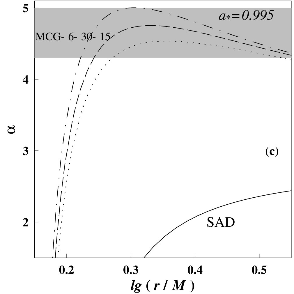
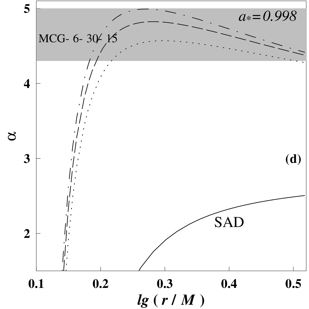
Figure 8: The emissivity index of the Seyfert 1 galaxy MCG-6-30-15 inferred from the observation of XMM-Newton is shown in the shaded region. The emissivity index of a standard accretion disk (SAD) is plotted in solid line. The emissivity index produced by MC process is plotted versus $\lg(r/M)$ in dotted, dashed and dot-dashed lines for $n=6.0,7.5$ and $9.2$ in (a), $n=4.3,\mbox{ 6}.0$ and $7.3$ in (b), $n=6.8,8.0$ and $9.5$ in (c), and $n=5.8,7.0$ and $7.8$ in (d), respectively. The following parameters are imposed: $\theta_{L}=0.40\pi$ in (a) and (b), $\theta_{L}=0.45\pi$ in (c) and (d); $a_{*}=0.995$ in (a) and (c), $a_{*}=0.998$ in (b) and (d).

Table 1: Direction of $\vec{S}_{L}^{p}$, $\vec{S}_{E}^{p}$ and corresponding quantities above and below EQP of the BH (EQP in Table 1 and Table 2 below is an abbreviation for equatorial plane)

Position	$\vec{B}^{p}$	$\vec{B}^{T}$	Current through $m$-loop	$\vec{S}_{L}^{p}\quad and\quad\vec{S}_{E}^{p}$
above EQP OMCR IMCR	From the BH to the disk	Opposite to $\vec{m}$ Same as $\vec{m}$	$I>0$, downwards $I<0$, upwards	From the BH to the disk From the disk to the BH
below EQP OMCR IMCR	From the disk to the BH	Same as $\vec{m}$ Opposite to $\vec{m}$	$I<0$, upwards $I>0$, downwards	From the BH to the disk From the disk to the BH

Table 2: Direction of $(\vec{S}_{E}^{p})_{1}$ and corresponding quantities above and below EQP of the BH

Case	$\vec{v}^{F}$	$\vec{E}^{p}$	$\vec{B}^{T}$	$(\vec{S}_{E}^{p})_{1}$
above EQP A B C $\Omega^{F}>\Omega^{H}>\omega$ $\Omega^{H}>\Omega^{F}>\omega$ $\Omega^{H}>\omega>\Omega^{F}$	Same as $\vec{m}$ Same as $\vec{m}$ Opposite to $\vec{m}$	Outward and normal to $\vec{B}^{p}$ Outward and normal to $\vec{B}^{p}$ Inward and normal to $\vec{B}^{p}$	Same as $\vec{m}$ Opposite to $\vec{m}$ Opposite to $\vec{m}$	Opposite to $\vec{B}^{p}$ Same as $\vec{B}^{p}$ Opposite to $\vec{B}^{p}$
below EQP D E F $\Omega^{F}>\Omega^{H}>\omega$ $\Omega^{H}>\Omega^{F}>\omega$ $\Omega^{H}>\omega>\Omega^{F}$	Same as $\vec{m}$ Same as $\vec{m}$ Opposite to $\vec{m}$	Outward and normal to $\vec{B}^{p}$ Outward and normal to $\vec{B}^{p}$ Inward and normal to $\vec{B}^{p}$	Opposite to $\vec{m}$ Same as $\vec{m}$ Same as $\vec{m}$	Same as $\vec{B}^{p}$ Opposite to $\vec{B}^{p}$ Same as $\vec{B}^{p}$

Table 3: The parameters $a_{*}$, $n$, and $\theta_{L}$ adapting the emissivity index to the observations

$\theta_{L}$	$a_{*}=0.990$	$a_{*}=0.992$	$a_{*}=0.994$	$a_{*}=0.996$	$a_{*}=0.998$
$0.40\pi$	$5.9-11.1$	$5.6-10.4$	$4.9-9.6$	$3.8-8.7$	$4.0-7.3$
$0.45\pi$	$6.4-11.3$	$6.1-10.6$	$5.8-9.9$	$5.3-9.0$	$4.1-7.8$
$0.48\pi$	$6.5-11.4$	$6.3-10.7$	$6.0-10.0$	$5.6-9.2$	$4.9-8.0$

References

- (1) Bardeen J. M., Press W. H., and Teukolsky S. A., 1972, ApJ, 178, 347
- (2) Blandford R. D., 1976, MNRAS, 176, 465
- (3) Blandford R. D., Znajek R. L., 1977, MNRAS, 179, 433
- (4) Blandford R. D., 1999, in Sellwood J. A., Goodman J., eds, ASP Conf. Ser. Vol. 160, Astrophysical Discs: An EC Summer School,Astron. Soc. Pac., San Francisco, p.265
- (5) Ghosh P., Abramowicz M. A., 1997, MNRAS, 292, 887
- (6) Li L. -X. 2000, ApJ, 533, L115
- (7) Li L. -X. 2002, ApJ, 567, 463 (Li02a)
- (8) Li L. -X. 2002, A&A, 392, 469 (Li02b)
- (9) Li L. -X. 2002, Phys. Rev. D, 65, 084047 (Li02c)
- (10) Li L. -X., Paczynski B., 2000, ApJ, 534, L 197
- (11) Macdonald D., Thorne K. S., 1982, MNRAS, 198, 345 (MT)
- (12) Wald R. M., 1984, General Relativity, Chicago Univ. Press, Chicago
- (13) Wang D. X., Xiao K., Lei W. H., 2002, MNRAS, 335, 655 (WXL)
- (14) Wang D. X., Lei W. H., Ma R. Y., 2003, MNRAS, (accepted, WLM)