A study of dark matter halos and gas properties in clusters of galaxies from ROSAT data.

Self-gravitating systems such as elliptical galaxies appear to have a constant integrated specific entropy and obey a scaling law relating their potential energy to their mass. These properties can be interpreted as due to the physical processes involved in the formation and evolution of these structures. Dark matter halos obtained through numerical simulations have also been found to obey a scaling law relating their potential energy to their mass with the same slope as for ellipticals, and very close to the expected value predicted by theory. Since the X-ray gas in clusters is weakly dissipative, we test here the hypothesis that it verifies similar properties. Comparable properties for the dark matter component are also investigated.
With this aim, we have analyzed ROSAT-PSPC images of 24 clusters, and fit a Sérsic law to their X–ray surface brightness profiles. We found that: 1) the Sérsic law parameters (intensity, shape and scale) describing the X-ray gas emission are correlated two by two, with a strong correlation between the shape and scale parameters; 2) the hot gas in all these clusters roughly has the same integrated specific entropy, although a second order correlation between this integrated specific entropy and both the gas mass and the dynamical mass is observed; 3) a scaling law links the cluster potential energy to its total mass, with the same slope as that derived for elliptical galaxies and for dark matter halo simulations. Comparable relations are obtained for the dark matter component. All these correlations are probably the consequence of the formation and evolution processes undergone by clusters of galaxies.

1 Introduction

Clusters of galaxies are known to be the largest gravitationally bound objects in the Universe. The amplification of primordial density fluctuations by gravity is thought to be the origin of structure formation, however the details of the formation process are not yet well understood and the study of the structure and properties of dark matter halos and of the intra cluster plasma in virialized systems can give important clues to understand the physics involved in the formation and evolution of galaxy clusters. Nowadays, these studies have undergone great improvements with the developement of advanced observational facilities and techniques, together with the progress of numerical simulations.

Many works have been developed during the last decades on this respect. Secondary infall and the effects of this process on the cluster structure were discussed by Gunn & Gott (1972), and self-similar solutions for dark matter halos and gas were studied in numerical simulations carried out e.g. by Fillmore & Goldreich (1984), Bertschinger (1985), Teyssier et al. (1997) and Subramanian (2000). Cold Dark Matter (CDM) studies based on high-resolution N-body simulations performed by Navarro, Frenk & White (1996, 1997) suggest a cuspy and universal dark matter (DM) density profile in galaxies and clusters of galaxies, independent of mass scale and cosmology; this result is contradicted by Jing & Suto (2000). However, some important observational facts seem not to be reproduced by these studies: numerical simulations based on the CDM scenario predict density profiles with steep inner slopes which fail to reproduce the rotation curves of low surface brightness (LSB) galaxies (Flores & Primack 1994; Moore et al. 1999). Although other works claim that cuspy DM profiles are consistent with the available data for dwarfs and LSB galaxies (van den Bosch & Swaters 2001), microlensing studies towards the center of our galaxy also support the incompatibility between CDM simulations and observational evidence (Binney & Evans 2001). To explain the discrepancy concerning the central slopes of DM halos (Navarro, Frenk & White 1997; Moore et al. 1999), the lack of sufficient resolution in the central regions of simulated halos has been proposed; Point Spread Function (PSF) effects together with insufficient resolution on galaxy rotation curves (van den Bosch & Swaters 2001) may be also at the origin of the discrepancy between models and observations.

Observations in the X-ray band provide valuable information on the hot Intra Cluster Medium (ICM). A popular model used to fit the spatial distribution of the X-ray gas is the so called $\beta$-model (Cavaliere & Fusco-Femiano 1976; Sarazin 1988) which assumes an isothermal ICM. However, this model may not be good enough to describe the cluster gas component, since the isothermality of the ICM is still rather controversial. Cooling flows are known to produce a drop of the gas temperature towards the center of the cluster; besides, outside the cooling flow region things are still not clear. Temperature profiles based on ASCA (White 2000) and ROSAT (Irwin, Bregman & Evrard 1999) data were found to be consistent with the isothermal hypothesis. On the other hand, Markevitch et al. (1998) found from ASCA observations that cluster temperatures decrease significantly with radius. Irwin & Bregman (2000) analysed BeppoSAX data and claimed a slight rise in cluster temperature with radius, a result which is at odds with De Grandi & Molendi (2002), who found that for a set of 21 clusters the temperature profile has a clear isothermal core (excluding the cooling flow region) followed by a rapid radial decline. Note that such a core is consistent with Chandra observations of cooling flow clusters, where the temperature profile rises rapidly with radius, then remains approximately constant out to $\sim$ 0.8 Mpc (Allen, Schmidt & Fabian 2001). Finally, XMM-Newton observations e.g. of Coma (Arnaud et al. 2001) and Abell 1795 (Tamura et al. 2001) show small but significant radial variations of the temperature. Numerical simulations seem to confirm a decline of temperature profiles with radius, but are not able to reproduce the flatness of these profiles in the innermost regions (Frenk et al. 1999; Loken et al. 2002). This disagreement may be due to additional physical processes that must be taken into account in future numerical simulations. Another point is that a single $\beta$ value cannot always fit the X-ray surface brightness profile of clusters (Allen, Ettori & Fabian 2001; Allen, Schmidt & Fabian 2001; Hicks et al. 2002).

The ICM density and temperature distributions are of fundamental importance because they can be used to determine the specific entropy distribution of the ICM, thus providing important information to understand nongravitational internal and external processes that may contribute to the ICM thermal history, such as external preheating and energy injection supernova-driven galaxy winds (Brighenti & Mathews 2001; Dos Santos & Doré 2002). Non-gravitational processes may be responsible for the observed breaking of the self-similar relation between X-ray luminosity and temperature predicted by theory (Arnaud & Evrard, 1999; Rosati, Borgani & Norman 2002 and references therein) and also the so called Entropy Floor (Ponman, Cannon & Navarro, 1999; Helsdon & Ponman 2000; Lloyd-Davies et al. 2000).

With the assumption that the X-ray plasma in clusters of galaxies is weakly dissipative, clusters considered as self-gravitating systems are likely to verify properties similar to those recently found in elliptical galaxies, considered as self-gravitating systems. Namely, the optical surface brightness profiles of elliptical galaxies can be fit by a Sérsic law (Sérsic 1968; Caon et al. 1993; Ciotti & Bertin 1999):

$$\Sigma(s)=\Sigma_{0}\>exp\left[-\left(\frac{s}{a}\right)^{\nu}\right]$$ (1)

characterized by three parameters: $\Sigma_{0}$ (intensity), $a$ (scaling) and $\nu$ (shape). For a sample of 132 ellipticals belonging to three galaxy clusters, the Sérsic parameters were found to be correlated two by two, and in the three-dimensional space defined by these three parameters they are located on a thin line. These properties have been interpreted as due to the fact that, to a first approximation, all these elliptical galaxies have the same specific entropy (entropy per unit mass) (Gerbal et al. 1997, Lima Neto et al. 1999, Márquez et al. 2000), and that a scaling law exists between the potential energy $U$ and the mass $M$ for these galaxies: $U\ \propto\ M^{1.72\pm 0.03}$ (Márquez et al. 2001). Each of these relations defines a two-manifold in the [$log\Sigma_{0},loga,\nu$] space. The thin line on which the galaxies are distributed in this space is the intersection of these two two-manifolds. Such relations are most probably a consequence of the formation and evolution processes undergone by these objects, since theory predicts $U\ \propto\ M^{5/3}$ under the hypothesis that energy and mass are conserved (Márquez et al. 2001).

Interestingly, numerical simulations of cold dark matter haloes in two different mass ranges lead to a similar scaling law between the potential energy and mass of the haloes. In the mass range $4\times 10^{5}\ \leq\ M\ \leq\ 4\times 10^{8}\ M_{\odot}$ (unvirialized clusters), Jang-Condell & Hernquist (2001) find a relation consistent with $U\ \propto\ M^{5/3}$, while in the mass range $10^{12}\ \leq\ M\ \leq\ 10^{15}\ M_{\odot}$ (virialized clusters) Lanzoni (2000) finds $U\ \propto\ M^{1.69\pm 0.02}$.

In this work, we present a study aimed at testing whether results similar to those found in elliptical galaxies can also be obtained for galaxy clusters, based on an accurate modeling of the cluster X-ray surface brightness. We use a de-projection of the Sérsic profile (Eq. 1) to obtain the gas and DM density distributions, temperature profiles, dynamical mass distributions and estimations of the integrated specific entropies of the gas and DM components for a set of 24 nearby galaxy clusters and a group. Interesting correlations between physical quantities are found, comparable to those observed in elliptical galaxies, which can give important clues to understand better the formation and evolution of galaxy clusters. This paper is structured as follows: our sample is described in Sect. 2; the calculations of the physical quantities used in this paper are presented in Sect. 3; the method used to determine the gas density profile from the X-ray surface brightness is described in Sect. 4; the methods used to derive the temperature profile and the dark matter distribution are explained in Sect. 5; results are presented in Sect. 6 and conclusions in Sect. 7.

2 The sample

We have retrieved data taken with the PSPC-B camera of ROSAT from the ROSAT archive at MPE. The energy range considered is 0.44$-$2 keV, corresponding to the four energy bands R4 to R7 (Snowden et al. 1994). These bands were chosen in order to avoid the low signal to noise ratio in the lower bands due to the high absorption by the hydrogen column. The spatial resolution of the PSPC is 25” and its energy resolution corresponds to 0.43% at 0.93 keV. We selected observations with the longest exposure times and where the cluster showed a regular shape, with no obvious mergers and a smooth light curve (no strong scattered solar X-ray contamination). We thus built a sample of 24 clusters (see Table 1) with redshifts ranging between $0.01$ and $0.3$. Redshifts were taken from the SIMBAD data base (except for A2199 for which the redshift was obtained from Wu, Xue & Fang 1999), and gas temperatures and luminosities from Wu, Xue & Fang (1999), except for A2034 and A2382 for which temperatures were taken from Ebeling et al. (1996). We assume $H_{0}=50\;\rm km\;s^{-1}\;Mpc^{-1}$, $\Omega_{0}=1$, and $\Lambda=0$ throughout this analysis. In order to increase the range in $T_{X}$, in particular to include cooler systems when drawing the $L_{X}-T_{X}$ relation, we intended to add several groups to our sample of clusters. However, we only included in our sample the group HCG 62, the one with the longest exposure time and best signal to noise ratio (we also tried to include HCG 94, but discarded it because of its signal to noise ratio). More groups will be considered in forecoming works.

The data reduction was done using the software developed by Snowden et al. (1994). The routines in the software provide the best available modeling and subtraction of various non-cosmic background components and corrections for exposure, satellite wobbling, vignetting and variations of detector quantum efficiency. A flat-field correction of the images was applied and the non-extended sources were masked, except the cluster centers. The whole procedure was carried out only in clusters without strong scattered solar X-ray contamination; for each cluster, we checked the light curves in the 4 energy bands considered, and all those with count rate peaks larger than 3 counts sec^-1 in their light curves were excluded.

Table 1: Cluster sample and observational data from the literature

$Cluster$	z	Exp. time (sec)	$T_{0}$ (keV)	$L_{X}(10^{44}$ erg s${}^{-1})$
A85	0.0518	10240	$6.20^{+0.40}_{-0.15}$	$19.52^{+1.35}_{-1.35}$
A478	0.0881	21969	$6.90^{+0.35}_{-0.35}$	$32.00^{+4.08}_{-4.08}$
A644	0.0704	10246	$6.59^{+0.17}_{-0.17}$	$18.92^{+2.17}_{-2.17}$
A1651	0.0860	7429	$6.10^{+0.20}_{-0.20}$	$18.78^{+2.21}_{-2.21}$
A1689	0.1810	13957	$9.02^{+0.40}_{-0.30}$	$55.73^{+8.92}_{-8.92}$
A1795	0.0631	26172	$5.88^{+0.14}_{-0.14}$	$25.42^{+1.47}_{-1.47}$
A2029	0.0765	12550	$8.47^{+0.41}_{-0.36}$	$41.93^{+2.96}_{-2.96}$
A2034	0.1510	8952	$7.00$	$6.86$
A2052	0.0348	6211	$3.10^{+0.20}_{-0.20}$	$4.27^{+0.34}_{-0.34}$
A2142	0.0899	6186	$9.70^{+1.30}_{-1.30}$	$61.12^{+3.95}_{-3.95}$
A2199	0.0299	40999	$4.10^{+0.08}_{-0.08}$	$7.09^{+0.25}_{-0.25}$
A2219	0.2250	11200	$12.40^{+0.50}_{-0.50}$	$64.56^{+6.96}_{-6.96}$
A2244	0.0970	2963	$8.47^{+0.43}_{-0.42}$	$25.32^{+2.14}_{-2.14}$
A2319	0.0559	3169	$9.12^{+0.15}_{-0.15}$	$39.74^{+2.17}_{-2.17}$
A2382	0.0648	17444	$2.90$	$0.91$
A2390	0.2310	10335	$11.10^{+1.00}_{-1.00}$	$63.49^{+14.87}_{-14.87}$
A2589	0.0416	7289	$3.70^{+1.30}_{-0.70}$	$3.42^{+0.38}_{-0.38}$
A2597	0.0852	7163	$4.40^{+0.40}_{-0.70}$	$15.37^{+1.79}_{-1.79}$
A2670	0.0761	17679	$4.45^{+0.20}_{-0.20}$	$4.97^{+0.92}_{-0.92}$
A2744	0.3080	13648	$11.00^{+0.50}_{-0.50}$	$62.44^{+14.41}_{-14.41}$
A3266	0.0594	13547	$8.00^{+0.30}_{-0.30}$	$16.48^{+0.64}_{-0.64}$
A3667	0.0552	12560	$7.00^{+0.60}_{-0.60}$	$22.70^{+4.20}_{-4.20}$
A3921	0.0960	11997	$4.90^{+0.55}_{-0.55}$	$10.92^{+1.52}_{-1.52}$
A4059	0.0460	5439	$3.97^{+0.12}_{-0.12}$	$5.78^{+0.54}_{-0.54}$
HCG62	0.0137	19639	$1.1^{+0.05}_{-0.05}$	$0.12$

For A2034 and A2382, the temperatures and X-ray luminosities were taken from Ebeling et al. (1996)
who do not provide error bars.

3 Estimating physical quantities

3.1 Gas density profile

The observed X-ray emission of the ICM is directly related to the gas distribution in the dark matter halo gravitational potential. Thus, in order to compare theory with observations, a description of the gas distribution is needed. Using a parameter-dependent model for the gas density profile, it is possible to re-construct the 3D X-ray emission of the cluster which, once projected and compared to the observations (Sect. 4), will allow us to derive the best set of values for the model parameters. We have chosen a 3D deprojection of a Sérsic profile (Sérsic 1968) to describe the gas distribution in clusters. This choice was motivated by the fact that we already used this profile to fit the optical surface brightness of elliptical galaxies, and computed all the physical quantities needed here, such as the entropy, potential energy, etc., as a function of the three Sérsic parameters (see Márquez et al. 2001 and references therein). Note that from a mathematical point of view, since the Sérsic profile has three parameters instead of two (compared to other models as for instance the $\beta$-model), the fitting process is more flexible. Besides, the fact that the volume integral of this profile does not diverge at large radii allows us to compute important quantities such as the total mass, potential energy and entropy of the system without any extra mathematical requirement such as a cutoff radius, for instance. Note also that the Sérsic law (Eq. (1)) is a non-homologous generalization of the de Vaucouleurs $R^{1/4}$ profile (de Vaucouleurs 1948). The 3D deprojection of such a profile corresponds to a generalized form of the Mellier-Mathez profile (Mellier & Mathez 1987) given by:

$$\rho_{gas}(r)=\rho_{0}\>{(r/a)}^{-p}\>\exp[-{(r/a)}^{\nu}]$$ (2)

where $\rho_{0}$ is the volume gas density associated to the central column density $\Sigma_{0}$ and the parameters $p$ and $\nu$ are related by the numerical approximation (Márquez et al. 2001):

$$p\simeq 1.0-0.6097\nu+0.05563{\nu}^{2}$$ (3)

which gives the best approximation to the Sérsic law when Eq. (2) is projected. The Sérsic profile defined by Eq. (1) corresponds to a surface mass density while Eq. (2) is the volume mass density. The condition that the mass obtained by integrating Eq. (1) must be equal to the mass obtained by integrating Eq. (2) implies:

$$\rho_{0}=\frac{1}{a}\>\Sigma_{0}\>\frac{\Gamma(\frac{2}{\nu})}{2\>\Gamma(\frac{3-p}{\nu})}$$ (4)

where $\Gamma(a)$ is the complete gamma function defined by $\Gamma(a)=\int^{\infty}_{0}x^{a-1}e^{-x}dx$.

3.2 Dark matter distribution and dynamical mass

Once the gas distribution is known, a reasonable hypothesis can be used to derive the dark matter distribution in the cluster. Previous works on X-ray clusters suggest a power law relation between the distributions of dark matter and gas (e.g. Gerbal et al. 1992; Durret et al. 1994). We will assume here a relative distribution of the DM and gas of the form $\rho_{DM}/\rho_{gas}=R(r)$, where $R(r)$ is a power law of the form:

$$R(r)=\kappa\left(\frac{r}{a}\right)^{-\alpha}$$ (5)

Under this hypothesis, the dark matter also follows a Sérsic law: it decreases exponentially above a certain radius and its asymptotic behavior towards the cluster centre is a power law of slope $p^{\prime}=-(p+\alpha)$. The values for $\kappa$, assuming $\alpha=0.25$ are given in Table 2 (see Sect. 4).

Using Eqs. (5) and (2), the total amount of mass contained within a spherical region of radius $r$ is given by the integral:

$$M_{Dyn}(r,\kappa,\alpha)=\int^{r}_{0}\left[\kappa\left(\frac{u}{a}\right)^{-\alpha}+1\right]\rho_{gas}(u)4\pi u^{2}\mathrm{d}u=$$

$$\frac{4\pi\rho_{0}a^{3}}{\nu}\left\{\kappa\ \gamma\left[\frac{3-(p+\alpha)}{\nu},\left(\frac{r}{a}\right)^{\nu}\right]+\gamma\left[\frac{3-p}{\nu},\left(\frac{r}{a}\right)^{\nu}\right]\right\}$$ (6)

where $\gamma(a,z)$ is the incomplete gamma function defined by $\gamma(a,z)=\int^{z}_{0}x^{a-1}e^{-x}dx$.

3.3 Gas temperature profile

An important point in our study is to compute the temperature distribution of the ICM. This can be achieved by estimating the gas density profile, obtained by fitting the observations, and assuming that clusters of galaxies are systems in a nearly hydrostatical equilibrium sate. A hypothesis on the state equation of the ICM gas is also needed. An ideal gas state equation can be considered as a good approximation, although its application to self-gravitating systems has been questioned in the past (see Bonnor 1956 and references therein).

Therefore, the equation of hydrostatical equilibrium:

$$\nabla P(r)=-G\frac{M_{Dyn}(r)}{r^{2}}\rho_{gas}(r)$$ (7)

is then combined with the equation of state for the hot intra-cluster plasma:

$$P(r)=\frac{\rho_{gas}(r)}{\mu m_{p}}k_{B}T_{gas}(r)\;$$ (8)

to provide the following equation from which the ICM temperature as a function of radius $T_{gas}(r)$ can be derived once the gas number density as a function of radius $n_{gas}(r)$ is known:

$$M_{Dyn}(r)=-\frac{k_{B}}{\mu m_{p}G}r^{2}\left\{T_{gas}(r)\frac{\mathrm{d}\,\ln[n_{gas}(r)]}{\mathrm{d}r}\right.+$$

$$+\left.\frac{\mathrm{d}T_{gas}(r)}{\mathrm{d}r}\right\}\;$$ (9)

where $G$ is the gravitational constant, $k_{B}$ is the Boltzman constant, $\mu$ is the plasma molecular weight (we assume $\mu=0.6$ for the ICM) and $m_{p}$ the proton mass. The electron number density and the gas mass density are related by $n_{gas}(r)=\rho_{gas}(r)/(1.14\ m_{p})$. The gas temperature profile can be obtained as a function of $\kappa$ and $\alpha$ by replacing Eqs. (6) and (2) into Eq. (9), and performing a Gauss-Laguerre integration of the latter. The solution is of the form:

$$T(r,\kappa,\alpha)=\left(\frac{w}{\nu a}\right)\left(\frac{r}{a}\right)^{p}e^{{\left(\frac{r}{a}\right)}^{\nu}}t(r,\kappa,\alpha)$$ (10)

where $w\equiv 4\pi\,G\,\frac{\mu m_{p}}{k_{B}}\,\frac{\rho_{0}a^{3}}{\nu}=1.54\times 10^{38}\left(\frac{\rho_{0}a^{3}}{\nu}\right)\ {\rm m\;keV}$, and

$$t(r,\kappa,\alpha)=\int^{\infty}_{\left(\frac{r}{a}\right)^{\nu}}\left\{\kappa\gamma\left[\frac{3-(p+\alpha)}{\nu},x\right]\right.+$$

$$+\left.\gamma\left[\frac{3-p}{\nu},x\right]\right\}x^{-\frac{(p+\nu+1)}{\nu}}e^{-x}\mathrm{d}x$$ (11)

Eq. (10) will be used together with a model for the hot plasma spectrum to derive the best set of values for $\kappa$ and $\alpha$, in agreement with quantities already observed in clusters of galaxies such as their mean X-ray temperature and luminosity and their baryonic mass fraction (see Sect. 5).

3.4 Potential energy and specific entropy

Changing the upper limit of the integral in Eq. (6) to $\infty$ we obtain the total dynamical mass:

$$M_{Dyn}=\frac{4\pi\rho_{0}a^{3}}{\nu}\left\{\kappa\,\Gamma\left[\frac{3-(p+\alpha)}{\nu}\right]+\Gamma\left(\frac{3-p}{\nu}\right)\right\}$$ (12)

The total potential energy of the cluster is given by:

$$U_{pot}=G\frac{M^{2}_{Dyn}}{R_{g}}$$ (13)

where the gravitational radius $R_{g}$ is defined by $R_{g}\>=\>a\>R^{*}_{g}$, where $a$ is the scale parameter and $R^{*}_{g}$ is a dimensionless radius given by the numerical approximation:

$$ln(R^{*}_{g})\>\simeq\>\frac{0.82032-0.92446\>\ln(\nu)}{\nu}\>+\>0.84543\;\;$$

(Márquez et al. 2001).

In spite of the X-ray emission, which is responsible in many cases for cooling flow processes affecting the equilibrium state of the cluster in the inner regions, we may consider clusters as structures where dissipating processes are negligible compared to their gravitational energy, thus settling into a nearly thermodynamic equilibrium at large scale. This can be inferred by a simple order of magnitude calculation: the potential energy of a cluster of mass $\sim 10^{15}M_{\odot}$ and radius $\sim$ 1 Mpc is about $8\times 10^{64}$ ergs. The energy lost through X-ray emission during a Hubble time ($\sim 2\times 10^{17}$ s) by a cluster of X-ray luminosity $\sim 10^{45}$ erg s^-1 is around $3\times 10^{62}$ ergs, a value which is almost 300 times smaller than its potential energy. We can therefore estimate the gas entropy of such a configuration.

The specific entropy of the intra-cluster gas can be computed from the distribution function in the phase space, $f(\mathbf{x},\mathbf{v})$, of the gas particles using the microscopic Boltzmann-Gibbs definition:

$$s=-\frac{\int f\>ln(f)\>d^{3}x\>d^{3}v}{\int f\>d^{3}x\>d^{3}v}$$ (14)

where the Boltzmann constant is $k_{B}=1$. Note that this expresion gives us the specific entropy of the entire system (gas or DM) because the integration covers the total volume in phase space. This definition then corresponds to an integrated specific entropy, and it will be referred to as ’global’ specific entropy. It is important to say that when we use the words ’integrated’ or ’global’ for the specific entropy, we are referring to this definition applied to the gas or DM separately and not to the sum of these two components.

To find the distribution function some simplifying hypotheses are needed. The first one is that our system is spherically symmetric, and the second one is that the velocity dispersion of the gas particles is isotropic (we neglect any possible rotation of the gas). Thus the distribution function $f$, depending explicitly only on the total energy, can be obtained from the density profile by an Abel inversion (Binney & Tremaine 1987). In this way, $f=f(\rho)$ and the integrated specific entropy can be computed numerically as a function of the Sérsic parameters only, providing a way to estimate the integrated specific entropy of the ICM from its surface brightness fit. It is important to emphasize here that the Boltzmann-Gibbs definition of the specific entropy makes no assumption on the equation of state, in particular the ideal gas equation for the ICM, and no assumption either on the validity of a hydrostatic equilibrium state of the system; this definition is therefore a general one since it only assumes spherical symmetry and an isotropic velocity dispersion tensor. Since the method we present here, based on the cluster X-ray surface brightness fitting, provides a good constrain on the gas density profile, this density profile, together with Eq. (14) can be used to obtain a good estimate of the global ICM specific entropy.

The specific entropy can also be obtained from the following set of equations (Balogh, Babul & Patton 1999):

$$s(r)=c_{v}\left\{ln\left[\frac{2\pi(\mu m_{p})^{8/3}K_{0}(r)}{h^{2}}\right]+\frac{5}{3}\right\}\;$$ (15)

and

$$K_{0}(r)=\frac{k_{B}T_{gas}(r)}{\mu m_{p}\rho_{gas}(r)^{2/3}}\;$$ (16)

where $c_{v}$ is the specific heat capacity at constant volume of the plasma. These widely used equations require, however, the following assumptions on the ICM : the gas is considered to be monoatomic and the equation of state for an ideal gas is supposed to hold. By knowing the ICM density and temperature distributions, Eqs. (15) and (16) can then be used (see Sect. 6.3) to compute the gas specific entropy profile for each cluster. Gas density profiles are obtained from the X-ray surface brightness fit (see Sect. 4) while temperature profiles are derived by assuming both the hydrostatic equilibrium condition and the ideal gas state equation for the ICM, as explained before. Since the physical quantities involved here are intensive, these equations cannot be integrated to derive the integrated specific entropy of the gas, and Eq. (14) will have to be used for this purpose.

The entropy is of fundamental importance to understand the effects of non-gravitational processes on the thermodynamical history of clusters. Previous studies refer to the gas entropy at $0.1r_{vir}$, where $r_{vir}$ is the cluster virial radius (e.g. Ponman, Cannon & Navarro, 1999; Lloyd-Davies, Ponman & Cannon 2000), while in this work we estimate the gas specific entropy for the entire cluster. Our calculations take into account all possible sources of heating and cooling, regardless of the distance to the centre, thus providing a good quantitative basis to which models can be compared in order to disentangle the different processes that affect the internal energy of the ICM during its history since the earlier epochs of the cluster formation.

We also notice that our assumption concerning the $\rho_{DM}/\rho_{gas}$ ratio (Eq. (5)) implies that the resulting DM density distribution is also Sérsic-like, with a central density distribution described by a power law varying as $r^{-(p+\alpha)}$. Under the hypothesis already stated concerning the distribution function of particles in phase space, we can in principle also compute the integrated specific entropy of the DM halo by using Eq. (14) and the DM density profile. Therefore the DM specific entropy is calculated numerically from the equation:

$$s=-\frac{1}{M}\int^{\Psi(0)}_{0}\frac{dM}{d\epsilon}lnf(\epsilon)d\epsilon\;,$$ (17)

which can be derived from Eq. (14), and where $\epsilon$ represents the binding energy, $M$ the total halo mass, and $\Psi$ the relative gravitational potential (see Magnard 2002).

4 Fitting method and density profile

Finding the gas density profile amounts to deriving the best set of values for the Sérsic parameters. This has required to fit the ROSAT images by a pixel-to-pixel method, which creates a three-dimensional model of the X-ray emission which is then projected by integration along the line of sight, taking into account the energy response and the point spread function of the detector. The result is a synthetical image which can be compared to the observation, and the best set of Sérsic parameters is obtained by successive iterations. The gas density profile defined by Eq. (2) is used to model the bremsstrahlung emission, and the free-bound and bound-bound X-ray emissions are taken into account. The code computes the X-ray emissivity $\epsilon_{\nu}$ in every point; it is then projected to obtain the surface brightness. This projected image is then convolved with the ROSAT point spread function (PSF), which varies as a function of position (and energy) on the detector. We have used in our fits a FWHM of 2 pixels which corresponds to the central PSPC PSF.

The cluster redshift and the mean gas temperature are required as input parameters. To obtain an initial guess for the free parameters in Eq. (2) we fit a Sérsic profile (Eq. (1)) to the X-ray surface brightness of each cluster. In order to stay as close as possible to our hypothesis of spherical symmetry, we selected clusters presenting the most round and uniform projected X-ray emission. However, this emission is not perfectly circular and due also to the fact that what we observe is always a projection on the plane of the sky of a three dimensional structure, we decided to take into account during the fitting process the ellipticity of the projected emission supposing also that all the clusters are oblate spheroids, i.e., that the third axis along the line of sight is a major axis. If $a$ is the semi–major axis, which also corresponds to the scale parameter in the Sérsic profile, and $b$ is the semi–minor axis, we define the ellipticity of the projected X-ray emission by $e=\sqrt{1-(b/a)^{2}}$. The ellipticity and semi-major axis position angle of the X-ray distribution are thus considered as free parameters for the fit and given as inputs for the code. The gas was assumed to be isothermal as a first approximation.

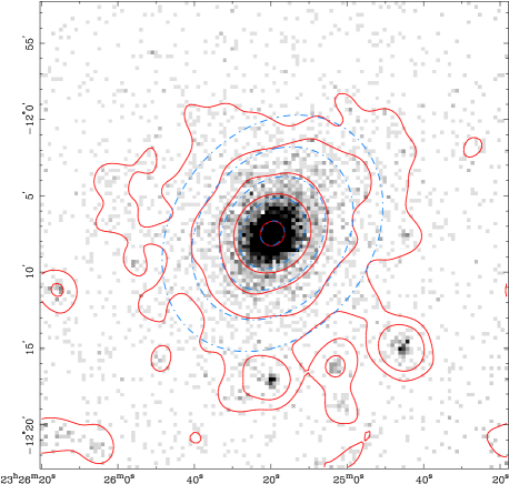
Figure 1: Comparison of our best model of the X-ray surface brightness (dot-dashed ellipses) with the corresponding ROSAT image for the cluster A2597. The X-ray iso-contours are 0.5, 1, 3, 10 and 100 times the background; they were made after smoothing the original image with a gaussian kernel of $\sigma=3.2$ pixels.

After obtaining the initial guesses for each free parameter, we use these values together with Eq. (2) to make a new synthetic image, then compare it to the actual ROSAT image. The parameter values are then changed and the comparison process is repeated iteratively, until it finds the 3D X-ray emission which best fits the surface brightness profile of the observation when projected. The fitting process is carried out with the MIGRAD method in the CERN MINUIT library (James 1994). In this process, the gas temperature is kept constant, as a first approximation. The exact shape of the temperature profile is not crucial when finding the set of values for the parameters, because the emissivity does not have a strong dependence on temperature as compared to its dependence on density; indeed, we find that modifying the temperature profile changes the values of the Sérsic parameters by at most a few percent, as explained in Sect. 5.

The fitting process directly gives us the best estimates for the semimajor axis $a$ and shape parameter $\nu$. However, the central electronic number density ${n_{e}}_{0}$ given by the fit is not accurate enough, and is estimated by another method (see Sect. 5).

We evaluated errors with the MINUIT error function MINOS, which calculates parameter errors taking into account both parameter correlations and non-linearities. Resulting errors correspond to a $1\sigma$ deviation.

All the equations presented in Sect. 3 refer to spherical symmetry, for which we had to define an equivalent scale parameter, $a_{eq}$ in order to go from the oblate geometry considered in the fit to the spherical geometry of the model. This new scale is defined as $a_{eq}=(a^{2}b)^{1/3}$ and will be used instead of $a$ to compute the specific entropy, the dynamical mass and the potential energy of a spherically symmetric X-ray region.

We show in Fig. 1 a comparison of our best fit Sérsic model of A2597. The good fit of the cluster surface brightness can clearly be seen, confirming the capability of the Sérsic profile to reproduce the cluster X-ray emission.

5 Gas temperature and dark matter to gas ratio

The fitting process described above provides the best values of $a_{eq}$ and $\nu$ for a given gas temperature profile, assuming as a first approximation that each cluster has an isothermal ICM, and then obtaining, through an iterative procedure, the best compatible gas density and non-isothermal temperature profiles, assuming hydrostatic equilibrium and spherical symmetry.

In order for the ${n_{e}}_{0}$ normalization to give the observed number of counts, we first computed the cluster flux $F$, after substraction of point sources and background (obtained by the 2D fit). The masked source pixel counts were set to the mean value taken within ellipses. Then ${n_{e}}_{0}$ was chosen so that a bremsstrahlung XSPEC model convolved by a hydrogen column absorption would give the same flux as seen by ROSAT:

$$F=\frac{3.02\times 10^{-15}}{4\pi d^{2}_{L}}\int n_{e}n_{I}dV=$$

$$\frac{3.02\times 10^{-15}}{4\pi d^{2}_{L}}\ \frac{2^{2+\frac{2p-3}{\nu}}}{\nu}a^{3}{{n_{e}}_{0}}^{2}\pi\Gamma\left[{\frac{3-2p}{\nu}}\right]$$

where $d_{L}$ is the luminosity distance to the cluster, and $n_{I}$ is the number density of plasma ions.

Eqs. (10) and (11) provide the ICM temperature profiles as families of solutions depending on the parameters $\kappa$ and $\alpha$. Since these are found to be different from those assumed to estimate the Sérsic parameters, the fitting process must be repeated, using the new temperature profile, in order to obtain a new set of parameters for each cluster, until convergence.

We tested on one cluster (A2029) the effect of a temperature gradient on the gas density profile from distances close to $r_{eff}/4$ outwards, where $r_{eff}$ corresponds to an effective radius which contains half of the cluster gas mass (see Table 2). For this, we did a second fit of the surface brightness of A2029 using a new temperature profile given by a power law of the form $T(r)=T_{0}(r/r_{eff})^{\beta}$ where $r_{eff}\simeq 2800$ kpc. $T_{0}$ was set in order to have a non-weighted mean temperature equal to the mean cluster temperature (Table 1) and we considered the cases $\beta=-0.5$ and $-1$. After the first iteration, the values found for ${n_{e}}_{0}$, $a_{eq}$, and $\nu$ remained almost unchanged for both values of $\beta$: the scale and shape parameters changed by about 1%, and the central electronic density by 4% with respect to the isothermal fit.

We therefore decided to keep the Sérsic values given by the original fit as the definitive ones. Eq. (10) can be re-written in the form $T(r,\kappa,\alpha)=\kappa T_{1}(r,\alpha)+T_{2}(r)$. We produced a set of $T_{1}(r,\alpha)$ profiles corresponding to values of $\alpha$ between 0 and 2 with steps of $\Delta\alpha=0.1$. These curves together with their corresponding $T_{2}(r)$ profiles and an adequate set of values for $\kappa$ were used to find which combination of $\kappa$ and $\alpha$ gives the closest values to the observed global temperatures and luminosities (Ebeling et al. 1996; Wu, Xue & Fang 1999), and baryon mass fractions (Arnaud & Evrard 1999; Mohr, Mathiesen & Evrard 1999; Schindler 1999). These quantities are evaluated as follows. The two profiles $n_{e}(r)$ and $T(r,\kappa,\alpha)$ plus the hypothesis of a gas metallicity equal to $0.3\,Z_{\odot}$ (see Renzini 1997) and the emission process determine the cluster X-ray emission. We used the XSPEC software to simulate the corresponding spectra with a bremsstrahlung emission model (to be coherent with the emission model used in the fitting program). We summed up the spectra from shells of constant electronic density and temperature over radius, considering only the volume intersected by the ROSAT observation cylinder. The spectrum obtained is then convolved with a photoelectric absorption model and with the ROSAT response function to produce the simulated spectrum. A fit is then performed on this spectrum to derive the X-ray temperature and luminosity (the metallicity and hydrogen column density are fixed).

The set of $\kappa$ and $\alpha$ has to produce $L_{X}$ and $T$ in agreement with the observed data within errors. Moreover, the gas mass fractions should stay inside the observed limits. So we performed a minimization of the distance between the observed data and the predictions from our model. We found that the best $\alpha$ is often very close to zero, which is not in good agreement with results obtained from numerical simulations by Teyssier (2002) which show a $\rho_{DM}/\rho_{g}$ ratio varying globally as $r^{-0.25}$; besides our values of $\alpha$ are not well constrained. We therefore chose to impose $\alpha=-0.25$; $\kappa$ was then recomputed to give luminosities and temperatures as close as possible to the observations.

To each temperature profile $T(r,\kappa,\alpha)$ corresponds a couple of simulated observational parameters $(T_{\rm sim},L_{\rm sim})$. The value of $\kappa$ is constrained by imposing these parameters to be close (within error bars) to the real observational values. The gas mass fraction is checked to be compatible with the isothermal hypothesis.

6 Results

6.1 Mass distributions and parameter correlations

The 3D gas density profiles were computed with Eq. (2) for all the clusters in our sample, using the sets of parameters obtained from the surface brightness fitting process (described in Sect. 4) of the PSPC images and listed in Table 2. By means of Eq. (5), the corresponding DM distribution can be recovered. In Fig. 2 we show the 3D gas and DM density profiles for every cluster divided by the critical density of the Universe at the cluster redshift (e.g., Ettori, De Grandi & Molendi 2002): $\rho_{c}(z)=3H^{2}(z)/(8\pi G)$, where the Hubble constant at redshift $z$ is defined by $H(z)=H_{0}\sqrt{\Omega_{m}(1+z)^{3}+1-\Omega_{m}}$.

Figure 2: 3D deprojected gas (full lines) and dark matter (dashed lines) density profiles divided by the critical density of the Universe at the cluster redshift.

Both DM and gas distributions are Sérsic-like, implying that the corresponding profiles decrease exponentially outwards above a certain distance from the cluster centre; on the other hand, when $r$ goes to zero they follow a power law in radius with a logarithmic slope tending asymptotically to $-p(\nu)$ for the gas and to $-(p(\nu)+\alpha)$ for the DM.

The values for $\kappa$, obtained as described in Sect. 5, are in most cases smaller than 10, while the value for $\alpha$ was fixed to 0.25 (see above). Although DM halos are denser than the ICM gas, as implied by the $\kappa$ factor and the asymptotic slope difference $\alpha$, the general shapes of both profiles look quite similar, implying that dark matter and gas are distributed in a comparable way. This effect is a natural consequence of the hypotheses and conditions imposed to our model. However such a behaviour seems to be the case for massive systems (like those in our sample - see total masses in Table 3), as shown by observations of galaxy clusters at moderate and high redshifts (Schindler 1999). The gas would be accreted into the forming structure and once the system reaches a relaxed state, the gas just accommodates into the halo potential. This is true at the scale of massive galaxy clusters where the potential well is deep enough to prevent the gas from expansion due to non-gravothermal processes. In this case, both dark matter and gas present similar distributions in contrast with what is observed in smaller systems such as groups of galaxies and even galaxies, where the gas can produce extended cores as result of energy injection due to supernova explosions or shock winds (Bryan 2000, Bower et al. 2001, Brighenti & Mathews 2001). It is also important to mention that Eq. (5), based on galaxy cluster observations, may no longer be valid for low mass systems such as groups of galaxies, in which case our DM model would be inappropriate to describe groups.

The averaged gas density profile for our set of 24 galaxy clusters is well fit by a Sérsic profile with parameters: $\rho_{0}=7.4\times 10^{-24}$ kg m^-3, $a_{eq}=367$ kpc and $\nu=0.56$. The latter gives $p(\nu)=0.67$ which makes the corresponding DM density profile vary as $r^{-0.92}$ when $r$ goes to zero. This central slope for the DM halo is shallower than the self-similar solution for spherical collapse in an expanding universe found by Bertschinger (1985) ($\rho\propto r^{-2.25}$), than the asymptotic behaviour found by Moore et al. (1999) in their numerical simulations ($\rho\propto r^{-1.5}$) and than the NFW (Navarro, Frenk & White, 1996, 1997) universal density profile. However it is steeper than the $\rho\propto r^{-0.75}$ critical solution found by Taylor & Navarro (2001) for galaxy-sized CDM halos based on the study of their phase-space density distribution. This critical solution can be interpreted as a maximally “mixed” configuration, where the phase-space distribution across the system is the most uniform one compatible with a monotonically decreasing density profile and with the power-law entropy distribution. This configuration would be the result of non-spherically symmetric formation processes through hierarchical merging. Mass shells are continously mixed and the density profiles tend to be shallower than the NFW profile at the center, converging to the $\rho\propto r^{-0.75}$ distribution for maximal mixing (Taylor & Navarro 2001).

One important advantage of the Sérsic density profile is that its volume integral converges when integrated up to infinity, making it thus possible to determine the total cluster mass, and the potential energy and entropy of the system without introducing a cutoff radius, in contrast to the popular $\beta$-model, for instance. Total dynamical masses can thus be computed (see Eq. (12)) and the resulting values for all clusters are given in Table 3.

Figure 3: Synthetic cumulative dynamical mass profiles normalized to the corresponding total integrated cluster mass $M_{Dyn}$. The radial coordinate is normalized to the cluster $r_{200}$ radius.

Fig. 3 shows the resulting cumulative dynamical mass profiles for every cluster as obtained by means of Eq. (6) with the corresponding Sérsic parameters. Every profile has been normalized to the corresponding cluster total mass, $M_{dyn}$ (see Eq. (12)), and the radial coordinate has been normalized to the corresponding cluster $r_{200}$ radius, which is defined as the radius within which the mean density is $200$ times the critical density of the universe, $\rho_{c}$, as defined above. In general, we can define a radius $r_{\Delta}$ within which the mean density is $\Delta$ times $\rho_{c}$ and $r_{\Delta}$ can be obtained from the relation $M(r<r_{\Delta})/(4\pi r^{3}_{\Delta}/3)=\Delta\rho_{c}$). The averaged cumulative dynamical mass distributions show a logarithmic slope $dlogM/dlogr\sim 1$ at $r\sim 0.7r_{200}$. Further out this slope decreases rather fast. According to our model, the cumulative mass profiles converge only around $r\sim 10r_{200}$, but the mass variation is only of a factor of two, going from $M\sim 10^{15}\ M_{\odot}$ at $\sim r_{200}$ to $M\sim 2\times 10^{15}\ M_{\odot}$ at $\sim 10r_{200}$.

The analysis by Ettori, De Grandi & Molendi (2002) of BeppoSAX data includes some clusters of our sample. They estimate masses for $\Delta=$ 1000 and 2500, by using either a NFW or a King profile for the total mass distribution. Comparing our results with theirs for same clusters, we see that our mass estimates, derived from the Sérsic profile for these two values of $\Delta$ within same $r_{\Delta}$ radii as indicated in their Table 2 are in quite good agreement. In most cases, our masses differ by about 10% or less, with differences reaching about 20% for a few cases. These differences are likely to be due to the use of different functional forms (the Sérsic, NFW and King models) to describe the mass profile. Moreover, from our sample we find in average $r_{200}\sim 2.5\pm 0.4$ Mpc (see Table 2). These values are about 78% of those found in numerical simulations by Navarro, Frenk & White 1996 for cluster sized systems of comparable masses. Moreover, we note that the values of our scale parameter $a_{eq}$ are comparable to those of the scale radius $r_{s}$ of the NFW profile for similar mass ranges. In this way, we obtain in average $a_{eq}/r_{200}\sim 0.12$ in good agreement with the value of $r_{s}/r_{200}\sim 0.14$ (Navarro, Frenk & White 1996), the difference being of only 14%. We can therefore say that the Sérsic profile is able to describe the mass distribution in clusters in as much the same way as other models as the NFW and King models, the differences being due to the mathematical natures of the models.

Based on a de-projected Sérsic model for the gas density profile, the best set of values of ${n_{e}}_{0}$, $a_{eq}$ and $\nu$ for each cluster is given in Table 2. These three parameters are displayed two by two in Figs. 4, 5 and 6. A clear correlation between the shape ($\nu$) and scale ($a_{eq}$) parameters is seen, while the correlations we find for $\Sigma_{0}-\nu$ and $\Sigma_{0}-a_{eq}$ ($\Sigma_{0}$ being obtained from $\rho_{0}$ by using Eq. (4)), are clear but show a somewhat larger scatter. Note that these three correlations have shapes similar to those found in elliptical galaxies. This may indicate, as for ellipticals, the existence of an entropic line on which galaxy clusters lie, in which case the correlation shown in Fig. 4 may just be the projection of this isentropic relation on the $log(\nu)-log(a_{eq})$ plane. In the case of elliptical galaxies, this entropic line was interpreted as the intersection of two surfaces in the [log $\Sigma_{0}$, log a, log $\nu$] space : the Entropic surface and the Energy-Mass surface (Márquez et al. 2001). In this work, we find that these two surfaces exist for our galaxy clusters as well, and these clusters are also located on a line corresponding to the intersections of the two surfaces (see Sect. 6.5). A complete discussion on this point will be presented in a forecoming paper (Magnard, in preparation). It is worth noting that, although from the mathematical point of view no correlation between the model parameters is expected, the fact that we observe such correlations probably indicates that they are due to the physics underlying the X-ray emission distribution.

Figure 4: Correlation between the density profile parameters $a_{eq}$ and $\nu$.

Figure 5: Correlation between the density profile parameters $\Sigma_{0}$ and $\nu$.

Figure 6: Correlation between the density profile parameters $\Sigma_{0}$ and $a_{eq}$.

Table 2: Best fit values for the Sersic parameters of the ICM, $\kappa$ from Eq. (5), and radius $r_{200}$ at which the mean density is 200 times the critical density of the Universe.

Cluster	$\nu$	$a_{eq}$ (kpc)	${n_{e}}_{0}\times 10^{-3}$ (cm${}^{-3})$	$\kappa$	$r_{200}$ (kpc)
A85	0.55$\pm$0.01	260$\pm$5	5.72$\pm$0.11	7.17$\pm$0.32	2714
A478	0.50$\pm$0.01	143$\pm$4	18.51$\pm$0.52	7.04$\pm$0.42	2607
A644	0.82$\pm$0.01	389$\pm$6	3.58$\pm$0.06	7.19$\pm$0.21	2421
A1651	0.74$\pm$0.02	385$\pm$9	3.57$\pm$0.11	6.59$\pm$0.25	2453
A1689	0.58$\pm$0.01	198$\pm$9	14.26$\pm$0.82	7.90$\pm$0.35	2594
A1795	0.54$\pm$0.00	164$\pm$2	12.30$\pm$0.23	7.64$\pm$0.21	2462
A2029	0.49$\pm$0.01	151$\pm$4	16.63$\pm$0.52	8.65$\pm$0.43	2946
A2034	1.00$\pm$0.03	811$\pm$18	1.72$\pm$0.04	3.58$\pm$0.43	2450
A2052	0.47$\pm$0.01	100$\pm$5	11.70$\pm$0.72	9.90$\pm$0.67	1930
A2142	0.81$\pm$0.01	528$\pm$6	3.86$\pm$0.05	4.26$\pm$0.50	2824
A2199	0.60$\pm$0.00	180$\pm$1	6.82$\pm$0.06	9.42$\pm$0.20	2142
A2219	0.85$\pm$0.02	689$\pm$15	3.40$\pm$0.08	4.04$\pm$0.24	2887
A2244	0.56$\pm$0.02	237$\pm$17	6.38$\pm$0.68	13.05$\pm$0.70	3039
A2319	0.80$\pm$0.01	755$\pm$13	1.86$\pm$0.04	5.13$\pm$0.10	3294
A2382	1.17$\pm$0.04	831$\pm$19	0.49$\pm$0.01	6.61$\pm$0.66	1900
A2390	0.59$\pm$0.02	313$\pm$16	8.61$\pm$0.48	5.13$\pm$0.62	2658
A2589	0.72$\pm$0.02	312$\pm$8	2.31$\pm$0.07	9.25$\pm$1.73	2008
A2597	0.39$\pm$0.01	37$\pm$4	71.44$\pm$46.76	12.42$\pm$1.60	2035
A2670	0.52$\pm$0.03	215$\pm$27	4.05$\pm$0.74	11.44$\pm$0.58	2331
A2744	1.35$\pm$0.07	877$\pm$25	2.26$\pm$0.07	4.82$\pm$0.29	2506
A3266	1.18$\pm$0.01	935$\pm$7	1.22$\pm$0.01	5.66$\pm$0.20	2973
A3667	0.89$\pm$0.01	990$\pm$9	1.07$\pm$0.01	3.29$\pm$0.36	2723
A3921	0.81$\pm$0.02	653$\pm$15	1.41$\pm$0.04	3.66$\pm$0.50	2090
A4059	0.64$\pm$0.01	233$\pm$8	4.34$\pm$0.18	8.46$\pm$1.02	2033
HCG62	0.36	22	17.4	36.9$\pm$1.63	$--$

6.2 Temperature profiles

We show in Fig. 7 the 3D non-weighted temperature profile for every cluster in our sample, calculated with the parameters given in Table 2 and normalized to the corresponding median temperature from the literature (see Table 1). As for the total mass profiles, the radial coordinate has been normalized to the corresponding cluster virial radius. All the profiles are very similar: they slightly increase from the center, then remain approximately constant to finally decrease at large radii. The mean temperature profile is consistent with an almost isothermal distribution for radii smaller than $0.25r_{200}$ ($\sim$ 625 kpc), in agreement with other works (Allen, Schmidt & Fabian 2001; De Grandi & Molendi 2002), followed by a rapid decrease for radii larger than $0.25r_{200}$, with a logarithmic slope of the order of $-0.6$ for radii around $0.63\ r_{200}$. This decrease results to be quite similar to the slope of $-0.64$ found by De Grandi & Molendi (2002) at radii larger than $\sim$ 750 kpc for their mean temperature profile, taking into account the cooling and non-cooling flow clusters of their sample. The results of Markevitch et al. (1998) based on ASCA observations show similar trends for the temperature distribution. The characteristic central drop we obtain in our temperature profiles is due to the mathematical properties of the density profile rather than to a real physical effect, but the lack of resolution of the PSPC impedes from properly addressing this issue, and we cannot tell anything about the temperature distribution within the central cooling flow region.

Figure 7: Synthetic 3 D temperature profiles calculated from Eqs. (10) and (11) with the values of $\alpha$ and $\kappa$ given in Table 2. The temperature is normalized to the global cluster temperature and the radial coordinate is normalized to the cluster $r_{200}$ radius.

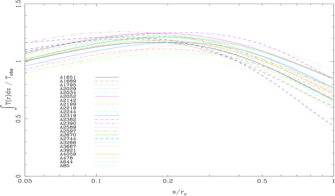
Figure 8: Re-projected emission weighted temperature deduced from our model. The projected radii $s$ are normalized to the corresponding $r_{v}=r_{200}$ radii, and the temperatures are normalized to the observed isothermal temperatures.

In Fig. 8 we show the re-projected emission weighted temperature profile for every cluster, defined by :

$$T_{\rm ew}(R)=\frac{\int n^{2}_{\rm e}(r)T(r){\rm d}z}{\int n^{2}_{\rm e}(r){\rm d}z}$$ (18)

Figure 9: Relation between $L_{X}$ and $T_{X}$. The point at the lower left corner corresponds to the group HCG 62. The solid line shows the best fit (see text) and the dotted line is the fit found by Markevitch (1998).

The $L_{X}-T_{X}$ relation derived from our calculations is shown in Fig. 9. Our power law fit (excluding HCG 62) is $L_{X}\propto T_{X}^{2.65\pm 0.17}$; the exponent is in agreement with Markevitch (1998), who finds $L_{X}\propto T_{X}^{2.64\pm 0.27}$, but our line is shifted towards higher luminosities. This shift is probably due to the fact that we include the central region in our luminosity evaluation, while Markevitch excises it.

6.3 ICM and DM specific entropies

Figure 10: Relation between the gas integrated specific entropy, $s_{gas}$ and the gas mass. The best fit line is indicated (see text).

Figure 11: Relation between the gas integrated specific entropy and the mean gas temperature taken from the literature (see text). The point at the lower left corner corresponds to the group HCG 62.

The global specific entropy $s_{gas}$ of the ICM is given in Table 3. It is found to vary very little from one cluster to another, as for the specific entropy of stars in elliptical galaxies (Márquez et al. 2001 and references therein). This is, however, a first order behavior. Numerical simulations of elliptical galaxies formed in a hierarchical merging scheme, show that their specific entropy varies a little with mass, most probably due to merging processes (Lima Neto et al. 1999, Márquez et al. 2000). The situation is not different in galaxy clusters. We show in Fig. 10 that the global specific entropy of the ICM and the gas mass are indeed clearly correlated, although this is a second order effect (about 2%), small compared to the dominant relation $s_{gas}\sim constant$ that we observe. The difference with elliptical galaxies is that the slope in Fig. 10 is steeper than for ellipticals: if we write $s_{gas}=s_{0}+\beta\ln(M_{gas})$, our best fit to the data gives $\beta=1.86\pm 0.15$ compared to $\beta\simeq 1$ for ellipticals (with $s_{0}$ constant). The error bars correspond to $1\sigma$ deviations and were computed from the parameter errors given by MINOS and by means of Monte Carlo simulations. Every parameter was modeled by a gaussian distribution with $\sigma$ equal to the corresponding $1\sigma$ deviation from MINOS. These distributions were then used to derive the total mass and specific entropy distributions and the corresponding $1\sigma$ errors for each cluster. For the linear fit we used a linear least-squares approximation in one dimension, taking into account the error bars in both directions at the same time. A comparable relation is found between the integrated specific entropy $s_{gas}$ of the ICM and the dynamical mass of the cluster, with a somewhat steeper slope of $2.67\pm 0.12$. In our fitting of the cluster X-ray surface brightness we have also taken into account the cluster center, thus our estimation of the gas specific entropy necessarily takes into account the effects of the central cooling flow. This information is integrated together with the other non-gravitational thermal processes affecting the intra cluster gas.

The integrated specific entropy of the X-ray gas is displayed in Fig. 11 as a function of the observed isothermal gas temperature. The entropy appears to increase with the temperature, consistently with a linear increase (the best fit to our data is shown in Fig. 11 and corresponds to $s_{gas}\propto T^{4.92}$). However, the dispersion is too large to assert a linear dependency. Note that such a relation has already been observed by Ponman et al. (1999) and Lloyd-Davies et al. (2000), and predicted by gravitational simulations (Borgani et al. 2001, Muanwong et al. 2002). The only group shown in this plot does not exhibit a significant entropy floor, but other groups need to be added. It would be important to get a good evaluation of this entropy floor as it is a strong constraint on the non-gravitational energy injection (Lloyd-Davies et al. 2000).

The derived gas density and temperature profiles can be used to compute the gas specific entropy profile for each cluster by using Eqs. (15) and (16).

Figure 12: $K_{0}$ profiles based on density and temperature models.

The $K_{0}(r)$ profiles are shown in Fig. 12, where the radial coordinate is normalized to the $r_{200}$ radius. All these profiles are consistent with a gas specific entropy increasing with radius, indicating that the gas has been heated by shock fronts at successive epochs when collapsing into the cluster potential well, before being virialized. Thus, the specific entropy profile provides useful information about the ICM thermal history. Some of the profiles present a clear steepening with radius at about $0.8\ r_{200}$, while others correspond to power laws throughout. The average of the profiles defined by Eq. (16) has a logarithmic slope $dlogK_{0}/dlogr\sim 1$ at about 0.6 $r_{200}$ and it is in agreement with results obtained by Tozzi & Norman (2001) who studied the effect of an entropy excess in the ICM gas before accretion into the DM halo. No entropy core is present, perhaps due to the effect of central cooling, although this could also be due to the mathematical nature of the profiles derived from the Sérsic model. In general our profiles are in agreement with external heating models for rich clusters (Tozzi, Scharf & Norman 2000; Tozzi & Norman 2001). However, we notice that the $K_{0}(r)$ profiles obtained from our density and temperature distributions are about a factor of 7 larger than those inferred by Tozzi & Norman (2001). This is probably just due to a normalization effect related to the way the density and temperature are computed; it is mainly the entropy variations that are a reliable physical quantity.

Figure 13: Relation between the dark matter integrated specific entropy and mass. The best fit line is indicated (see text).

The assumed relation (5) between the dark matter and gas densities allows us to also compute the global dark matter entropy (see Table 3) numerically from Eq. (17), which comes out directly from the definition given in Eq. (14). The corresponding entropy–mass relation thus found for the dark matter is very close to that obtained for the gas, with $\beta\simeq 1.90\pm 0.17$ as seen in Fig. 13.

Table 3: Gas and dynamical masses, potential energy, central gas column density and integrated specific entropy for gas and DM as derived from Sérsic parameters.

Cluster	M${}_{gas}(\times 10^{14}M_{\odot})$	$M_{Dyn}(\times 10^{15}M_{\odot})$	$U_{pot}\times 10^{58}$ (kg m2 s${}^{-2})$	$\Sigma_{0}$ (kg m${}^{-2})$	Gas Spec. Entr.	DM Spec. Entr.
A85	5.11$\pm$0.41	2.59$\pm$0.35	0.78$\pm$0.20	0.36$\pm$0.01	204.3$\pm$0.18	206.1$\pm$0.91
A478	4.98$\pm$0.56	2.29$\pm$0.35	0.72$\pm$0.21	0.68$\pm$0.03	204.1$\pm$0.24	205.7$\pm$1.00
A644	1.80$\pm$0.13	1.18$\pm$0.16	0.39$\pm$0.10	0.26$\pm$0.01	201.3$\pm$0.15	203.7$\pm$0.87
A1651	2.53$\pm$0.29	1.46$\pm$0.24	0.46$\pm$0.14	0.27$\pm$0.01	202.3$\pm$0.25	204.4$\pm$0.98
A1689	4.11$\pm$0.85	2.35$\pm$0.52	1.05$\pm$0.41	0.65$\pm$0.05	203.3$\pm$0.43	205.3$\pm$1.22
A1795	3.10$\pm$0.20	1.63$\pm$0.20	0.45$\pm$0.10	0.50$\pm$0.01	203.0$\pm$0.14	204.9$\pm$0.88
A2029	6.14$\pm$0.69	3.26$\pm$0.46	1.26$\pm$0.31	0.66$\pm$0.03	204.6$\pm$0.25	206.5$\pm$1.00
A2034	4.44$\pm$0.44	1.79$\pm$0.42	0.64$\pm$0.29	0.23$\pm$0.01	203.1$\pm$0.22	204.6$\pm$0.93
A2052	1.67$\pm$0.38	0.95$\pm$0.21	0.13$\pm$0.05	0.32$\pm$0.02	202.4$\pm$0.49	204.3$\pm$1.31
A2142	5.11$\pm$0.22	2.17$\pm$0.40	0.94$\pm$0.35	0.38$\pm$0.01	203.4$\pm$0.09	205.0$\pm$0.80
A2199	1.27$\pm$0.04	0.86$\pm$0.08	0.18$\pm$0.03	0.28$\pm$0.01	201.2$\pm$0.07	203.5$\pm$0.79
A2219	8.55$\pm$0.85	3.56$\pm$0.75	2.17$\pm$0.89	0.42$\pm$0.01	204.4$\pm$0.22	205.9$\pm$0.94
A2244	3.92$\pm$1.45	3.33$\pm$1.15	1.53$\pm$0.88	0.36$\pm$0.05	203.7$\pm$0.75	206.4$\pm$1.60
A2319	7.45$\pm$0.62	3.64$\pm$0.63	1.79$\pm$0.61	0.26$\pm$0.01	204.5$\pm$0.19	206.4$\pm$0.90
A2382	0.96$\pm$0.01	0.67$\pm$0.11	0.11$\pm$0.03	0.06$\pm$0.01	200.4$\pm$0.22	202.9$\pm$0.91
A2390	9.06$\pm$2.17	3.72$\pm$1.01	1.78$\pm$0.85	0.62$\pm$0.05	205.0$\pm$0.51	206.5$\pm$1.31
A2589	0.97$\pm$0.12	0.73$\pm$0.11	0.13$\pm$0.04	0.15$\pm$0.01	200.6$\pm$0.28	203.2$\pm$1.00
A2597	2.30$\pm$2.14	1.26$\pm$1.13	0.22$\pm$0.49	0.78$\pm$0.52	203.1$\pm$1.69	204.9$\pm$1.94
A2670	2.86$\pm$2.09	2.03$\pm$1.35	0.46$\pm$0.59	0.22$\pm$0.05	203.6$\pm$1.24	206.0$\pm$2.18
A2744	4.00$\pm$0.52	2.20$\pm$0.47	1.36$\pm$0.55	0.26$\pm$0.01	202.3$\pm$0.28	204.4$\pm$0.95
A3266	3.33$\pm$0.11	2.03$\pm$0.31	0.92$\pm$0.28	0.17$\pm$0.01	202.4$\pm$0.07	204.7$\pm$0.77
A3667	6.93$\pm$0.31	2.52$\pm$0.57	0.83$\pm$0.38	0.19$\pm$0.01	204.4$\pm$0.10	205.7$\pm$0.81
A3921	3.53$\pm$0.40	1.34$\pm$0.31	0.29$\pm$0.13	0.17$\pm$0.01	203.1$\pm$0.25	204.5$\pm$0.98
A4059	1.24$\pm$0.20	0.80$\pm$0.14	0.15$\pm$0.05	0.22$\pm$0.01	201.2$\pm$0.34	203.5$\pm$1.09

6.4 Potential energy – mass relation

Figure 14: Relation between the dynamical mass and the potential energy. The solid line corresponds to the best fit to the data and the dashed line is the theoretical slope of $I=5/3$ defined by the relation $ln(U_{pot})-I\ ln(M_{dyn})=const$.

The relation between the dynamical mass and potential energy, previously shown for elliptical galaxies (Márquez et al. 2001) and in numerical simulations (Lanzoni, 2000; Jang-Condell & Hernquist, 2001), is displayed in Fig. 14 for our set of clusters. If we write it as $ln(U_{pot})-I\,ln(M_{dyn})=const$, the best fit to our data imply $I=1.68\pm 0.08$, in excellent agreement with the theoretical value of $5/3$. The error bars and linear fit are computed in the same way as explained in the previous section.

6.5 Discussion

The correlations presented in the previous sections between the mass, potential energy and integrated specific entropy, confirm the existence of an entropic surface, $s(\Sigma_{0},a,\nu)-\beta\ ln(M(\Sigma_{0},a,\nu))=const$ (see Eq. (14)), and a potential energy-mass surface, $ln(U_{pot}(\Sigma_{0},a,\nu))-I\ ln(M_{dyn}(\Sigma_{0},a,\nu))=const$, in the Sérsic parameters space, remarkably similar to the case of elliptical galaxies (Márquez et al. 2001). Indeed, we observe the clusters in our sample to be located at the intersection of these two surfaces, indicating the existence of an “entropic line” for galaxy clusters (see Magnard 2002). We have checked by simulations that this line is also recovered for a random set of values of the Sérsic parameters, suggesting the possibility that this relation could be a consequence of the model assumed to describe the final viralized system (in our case a Sérsic profile). However, the fact that a Sérsic profile reproduces very well the X-ray surface brightness of clusters, and hence the gas distribution of the ICM, supports the idea that the physical processes operating during the formation and evolution of galaxy clusters, which are of course responsible for the final structure reached by the ICM and DM halo, are indeed at the origin of the entropic line. To confirm this, the same method as in this work, but with different models for the gas density profile should be used. Moreover, the existence of both an entropic surface and a potential energy-mass surface for galaxy clusters implies that these objects can be considered as a single-parameter family, described by one of the Sérsic parameters only (e.g. Márquez et al. 2001). Interestingly, analogous correlations have been obtained for galaxy clusters by Fujita & Takahara (1999). The importance of the above mentioned correlations resides in the fact that they are probably the result of the physics ruling cluster formation. A correlation between the global specific entropy and the mass conserves information on the various events affecting the thermodynamical history of clusters. The observed variation of $s_{gas}$ with dynamical mass in clusters suggests that dissipating processes in clusters play an important role as generators of entropy. These mainly correspond to Bremsstrahlung emission ($L\propto M^{4/3}$) and cooling flows. Merging processes between clusters are of importance in such a relation, because of their impact on the final total mass and on the amount of entropy produced during the cluster formation. Violent merger events can be accompanied by an important dissipation of energy and creation of entropy, while minor mergers can be translated in an adiabatic accretion of matter without a significant production of entropy. These energy losses, however, are all negligible compared to the cluster gravitational energy. Thus the value of the slope $\beta$ in the specific entropy-mass relation reflects the impact of such processes on the cluster history. Clusters with higher global specific entropy could have undergone more episodes of hierarchical merging through their histories, thus becoming more massive.

On the other hand, considering the collapse of matter to form a virialized gravitational system, the correlation between the potential energy and the total mass of the final structure is a natural consequence of the conservation of energy and mass during its formation. A self-similar relation defined by $U\propto M^{5/3}$ is expected from theory (see Márquez et al. 2001) and we show that it is indeed also followed by our observed galaxy clusters.

All these results strongly suggest that the formation processes affecting galaxies and clusters of galaxies are quite similar regardless the scale involved.

7 Conclusions

We have shown in the present work that the Sérsic profile can be used as a good tracer of the matter distribution in clusters, under the assumption that clusters are well relaxed structures, as it was the case in elliptical galaxies. Its mathematical properties make it an interesting and useful tool that can be employed to explore the physics of relaxed systems, although any other appropriate profile can be used. The density profiles obtained here reproduce well the X-ray surface brightness profiles of the ROSAT PSPC images. The asymptotic behaviour of these profiles towards the cluster center turns out to be shallower than the NFW profile, but still within the limits predicted by numerical simulations concerning the central slope of galaxy-sized DM halos. Temperature profiles derived here (considering the hydrostatical equilibrium hypothesis for the cluster structure) are in agreement with other works. We estimate the integrated specific entropy content for galaxy clusters and our specific entropy profiles are consistent with the predicted shape of the entropy distribution for massive clusters, obtained by simulations which take into account pre-heating and cooling processes.

We have shown that both for the gas and for the dark matter the integrated specific entropy and the potential energy have behaviors comparable to those observed for stars in elliptical galaxies: the integrated specific entropy is constant to first order and in reality increases slightly with mass as a logarithmic function, while the potential energy scales with mass as a power law. Note that the index of this power law is close to the theoretical value of 5/3 for elliptical galaxies and clusters. This strongly suggests that all these self gravitating systems behave similarly, even though they may have very different masses and thermodynamical histories. Elliptical galaxies could then be considered as scaled down versions of galaxy clusters (Moore et al. 1999). Moreover, integrated specific entropy-mass and potential energy-mass correlations should be the result of the formation history of the clusters. Heating mechanisms and merger events play an important role here and total mass and energy are conserved during the whole formation process of the final virialized structure.

It would be interesting to apply the Sérsic model to high redshift galaxy clusters in order to test the possible evolution of the scaling relations found in this work. The use of Chandra and XMM-Newton data will be crucial in these kinds of studies due to their higher resolution and sensitivity compared to ROSAT. We also note that a similar analysis could be carried out in samples of synthetic clusters derived from numerical simulations.

- (1) Allen S., Ettori S. & Fabian A. 2001, MNRAS 324, 877
- (2) Allen S., Schmidt R. & Fabian A. 2001, MNRAS 328, L37
- (3) Arnaud M., Aghanim N., Gastaud R. et al. 2001, A&A 365, L67
- (4) Arnaud M. & Evrard A. 1999, MNRAS 305, 631
- (5) Balogh M. L., Babul A. & Patton D. R. 1999, MNRAS 307, 463
- (6) Bertschinger E. 1985, ApJS, 58, 39
- (7) Binney J. & Evans N. 2001, MNRAS 327, L27
- (8) Binney J. & Tremaine S. 1987, “Galactic Dynamics”, Princeton University Press
- (9) Bonnor W. B. 1956, MNRAS, 116, 351
- (10) Borgani S., Governato F., Wadsley J. et al. 2001, ApJL 559, L71
- (11) Bower R.G., Benson A.J., Lacey C.G. et al. 2001, MNRAS 325, 497
- (12) Brighenti F. & Mathews W. 2001, ApJ 553, 103
- (13) Bryan G. 2000, ApJ 544, L1
- (14) Caon N., Capaccioli M. & D’Onofrio M. 1993, MNRAS 265, 1013
- (15) Cavaliere A. & Fusco-Femiano R. 1976, A&A 49, 137
- (16) Ciotti L. & Bertin G. 1999, A&A 352, 447
- (17) de Vaucouleurs G. 1948, Ann. d’Astroph. 11, 247
- (18) De Grandi S. & Molendi S. 2002, ApJ 567, 163
- (19) Dos Santos S. & Doré O. 2002, A&A 383, 450
- (20) Durret F., Gerbal D., Lachièze-Rey M., Lima Neto G.B. & Sadat R. 1994, A&A 287, 733
- (21) Ebeling H., Voges W., Böhringer H. et al. 1996, MNRAS 281, 799
- (22) Ettori S., De Grandi S. & Molendi S. 2002, A&A 391, 841
- (23) Fillmore J. & Goldreich P. 1984, ApJ 281, 1
- (24) Flores R. & Primack J. R. 1994, ApJ 427, L1
- (25) Frenk C. S., White S.D.M., Bode P. et al. 1999, ApJ 525, 554
- (26) Fujita Y. & Takahara F. 1999, ApJ 519, L51
- (27) Gerbal D., Durret F., Lima Neto G.B., Lachièze-Rey M. 1992, A&A 253, 77
- (28) Gerbal D., Lima Neto G. B., Márquez I., Verhagen H. 1997, MNRAS 285, L41
- (29) Gunn J. & Gott J. R. III 1972, ApJ 176, 1
- (30) Helsdon S.F. & Ponman T.J. 2000, MNRAS 315, 356
- (31) Hicks A., Wise M., Houck J. & Canizares C. 2002, ApJ 580, 763
- (32) Irwin J.A., Bregman J.N. & Evrard A. E. 1999, ApJ 519, 518
- (33) Irwin J.A. & Bregman J.N. 2000, ApJ 538, 543
- (34) James F. 1994, CERN Program Library Long Writeup D506
- (35) Jang-Condell H. & Hernquist L. 2001, ApJ 548, 68
- (36) Jing Y. P. & Suto Y. 2000, ApJ 529, L69
- (37) Lanzoni B., 2000, PhD Thesis, Université Paris 7
- (38) Lima Neto G. B., Gerbal D., Márquez I. 1999, MNRAS 309, 481
- (39) Lloyd-Davies E.J., Ponman T.J. & Cannon D.B. 2000, MNRAS 315, 689
- (40) Loken C., Norman M.L., Nelson E. et al. 2002, ApJ 579, 571
- (41) Magnard F. 2002, PhD Thesis, Université Paris 6
- (42) Markevitch M., Forman W. R., Sarazin C. L. & Vikhlinin A. 1998, ApJ 503, 77
- (43) Markevitch M. 1998, ApJ 504, 27
- (44) Márquez I., Lima Neto G.B., Capelato H., Durret F., Gerbal D. 2000, A&A 353, 823
- (45) Márquez I., Lima Neto G.B., Capelato H. et al. 2001, A&A 379, 767
- (46) Mellier Y. & Mathez G. 1987, A&A 175, 1
- (47) Mohr J. J., Mathiesen B., Evrard A. E. 1999, ApJ 517, 627
- (48) Moore B., Quinn T., Governato F., Stadel J. & Lake G. 1999, MNRAS 310, 1147
- (49) Muanwong O., Thomas P. A., Kay S. T. & Pearce F. R. 2002, MNRAS 336, 527
- (50) Navarro J., Frenk C. & White S. 1996, ApJ 462, 563
- (51) Navarro J., Frenk C. & White S. 1997, ApJ 490, 493
- (52) Ponman T. J., Cannon D. B. & Navarro J. F. 1999, Nature, 397, 135
- (53) Renzini A. 1997, ApJ 488, 35
- (54) Rosati P., Borgani S., Norman C. 2002, ARA&A 40, 539
- (55) Sarazin C. 1988, “X-Ray Emission from Clusters of Galaxies”, Cambridge University Press
- (56) Schindler S. 1999, A&A 349, 435
- (57) Sérsic J. L. 1968, Atlas de Galaxias Australes, Observatorio Astronómico de Córdoba, Argentina
- (58) Snowden S. L., McCammon D., Burrows D.N., Mendenhall J.A. 1994, ApJ 424, 714
- (59) Subramanian K. 2000, ApJ 538, 517
- (60) Tamura N., Kaastra J.S., Peterson J.R. et al. 2001, A&A 365, L87
- (61) Taylor J. E. & Navarro J. F. 2001, ApJ 563, 483
- (62) Teyssier R., Chièze J.-P. & Alimi J.-M. 1997, ApJ 480, 36
- (63) Teyssier R. 2002, A&A 385, 337
- (64) Tozzi P., Scharf C. & Norman C. 2000, ApJ 542, 106
- (65) Tozzi P. & Norman C. 2001, ApJ 546, 63
- (66) van den Bosch F. C. & Swaters R. A. 2001, MNRAS 325, 1017
- (67) White D. 2000, MNRAS 312, 663
- (68) Wu X.-P., Xue Y.-J, Fang L.-Z. 1999, ApJ 524, 22