Separating E from B

Abstract

In a microwave background polarization map that covers only part of the sky, it is impossible to separate the $E$ and $B$ components perfectly. This difficulty in general makes it more difficult to detect the $B$ component in a data set. Any polarization map can be separated in a unique way into “pure $E$,” “pure $B$,” and “ambiguous” components. Power that resides in the pure $E$ ($B$) component is guaranteed to be produced by $E$ ($B$) modes, but there is no way to tell whether the ambiguous component comes from $E$ or $B$ modes. A polarization map can be separated into the three components either by finding an orthonormal basis for each component, or directly in real space by using Green functions or other methods.

1 Introduction

Detailed characterization of the polarization of the cosmic microwave background (CMB) radiation will be one of the main frontiers in cosmology in the coming years. The first detection of CMB polarization [1, 2] and the first measurement of the large-angle correlation between polarization and temperature [3, 4] have already taken place, and numerous experiments in the present and near future [5, 6, 7, 8, 9] will surely provide a wealth of polarization data.

A CMB polarization map consists of maps of the Stokes parameters $Q$ and $U$. The Stokes parameters are of course coordinate-dependent objects: $Q+iU$ is a spin-2 field. A key insight in CMB polarization theory is that the most natural way to express such a spin-2 field is to decompose it into scalar and pseudoscalar pieces, generally called $E$ and $B$ [10, 11]. This $E$/$B$ decomposition is crucial in analyzing polarization data. In particular, scalar perturbations (such as density variations) produce only $E$-type polarization (in linear theory), so detection of a $B$ component could provide evidence for vector or tensor perturbations. The search for the $B$ component is therefore likely to be of enormous importance: this component is capable of telling us about tensor (gravity-wave) perturbations produced during inflation [12, 13], probing the inflationary epoch far more directly than any other observations.

In standard models, the $B$ component is considerably weaker than the $E$ component, and so is likely to be difficult to detect [14]. To make matters worse, the $E$/$B$ decomposition is unique only for a full-sky map. This means that in the absence of complete sky coverage, unless one is very careful, $E$/$B$ confusion can reduce the detectability of the $B$ component [15, 16].

One way to quantify the problem of $E$/$B$ leakage is to observe that the space of all possible polarization maps over any given region of sky can be decomposed into three orthogonal subspaces: a “pure $E$” subspace, in which all power is guaranteed to come from $E$ modes, a “pure $B$” subspace, in which all power is guaranteed to come from $B$ modes, and an “ambiguous” subspace, in which there is no way to tell whether the power came form $E$ or $B$. This decomposition was worked out in spherical harmonic space for a spherical cap in [17], and the general formalism is described in [18]. In the latter work, explicit recipes are given for finding orthonormal bases (“normal modes”) for all three subspaces as eigenfunctions of the bilaplacian operator on the observed region. Furthermore, in the case of a pixelized map, we give an efficient way of finding approximately pure and ambiguous modes by solving a discrete eigenvalue problem.

An understanding of the $E$/$B$/ambiguous (hereinafter E/B/A) decomposition is likely to be of great importance in designing future experiments. For instance, the presence of ambiguous modes significantly increases the optimal sky coverage for a degree-scale $B$-detection experiment [16].

2 E and B modes

Figure 1: Left panel: An $E$ Fourier mode. Center panel: A $B$ Fourier mode. Right panel: An $E$ “hot spot.”

We begin by summarizing some fundamental properties of $E$- and $B$-type polarization maps. For further details, see [18]. Suppose for the moment that we have a polarization map that covers a small enough patch of sky to allow the use of the flat-sky approximation. In this case, it is natural to work in Fourier space, where the separation into $E$ and $B$ is quite simple. As shown in Figure 1, a Fourier mode is an $E$ mode if the polarization direction is parallel / perpendicular to the wavevector and is a $B$ mode if the polarization direction makes a 45^∘ angle with the wavevector. Any $E$ polarization map is a superposition of such $E$ Fourier modes; an example is the $E$ “hot spot” shown in the right panel of Figure 1. (To get a $B$ spot, simply rotate the polarization by 45^∘ at each point.) Realizations of $E$- and $B$-type Gaussian random fields are shown in Figure 2.

The Fourier-space description of the $E$/$B$ decomposition is very helpful in developing an intuitive understanding of the mixing of $E$ and $B$ modes in an incomplete or pixelized map. In a map that covers only part of the sky (say of size $L$), we can achieve resolution $\sim L^{-1}$ in $k$ space. That is, our estimate of a Fourier mode with wavevector ${\bf k}$ will actually include contributions with a range of wavevectors centered on ${\bf k}$ with a spread of $\sim L^{-1}$. Since wavenumbers with different directions will be mixed together, and since the direction of the wavevector is crucial to the $E$/$B$ separation, mixing is inevitable, with the worst problems occurring on the largest scales probed ($k\sim L^{-1}$).

In a pixelized map, problems crop up on the small-scale end as well, due to aliased power. When a mode with a wavevector ${\bf k}$ beyond the Nyquist frequency is aliased to a lower frequency, it typically is mapped into a mode whose wavevector points in a completely different direction. As a result, aliased power has nearly complete $E$/$B$ mixing. For this reason, avoiding aliasing (by oversampling the beam) is even more important in polarization experiments than in temperature experiments.

Figure 2: Gaussian random maps. One is an $E$ map; one is a $B$ map. For the reader who wishes to test his or her ability to tell $E$ from $B$, we reveal which is which in the references [19].

In real space, the two types of polarization maps satisfy differential equations on $Q$ and $U$. Any $E$ map must satisfy

$${\bf D}_{B}^{\dagger}\cdot{\bf P}=0,$$ (1)

where ${\bf P}=\left(\matrix{Q\cr U}\right)$ is the polarization map, and the differential operator ${\bf D}_{B}$ is

$${\bf D}_{B}=\left(\matrix{2\partial_{x}\partial_{y}\cr\partial_{x}^{2}-\partial_{y}^{2}}\right).$$ (2)

Note that the operator ${\bf D}_{B}$ acts on a scalar function to produce a two-component polarization “vector” $\left(\matrix{Q\cr U}\right)$, while the conjugate operator ${\bf D}_{B}^{\dagger}$ turns a polarization vector into a scalar.

Similarly, any $B$ map must satisfy ${\bf D}_{E}^{\dagger}\cdot{\bf P}=0$, with

$${\bf D}_{E}=\left(\matrix{\partial_{x}^{2}-\partial_{y}^{2}\cr-2\partial_{x}\partial_{y}}\right).$$ (3)

The easiest way to see that these equations are true is to verify that they work for arbitrary $E$ and $B$ Fourier modes.

In building intuition about $E$ and $B$ modes, it is extremely helpful to bear in mind the analogy with vector fields: an $E$ mode is the spin-2 analogue of a curl-free vector field, and a $B$ mode is the analogue of a divergence-free vector field. This means that the operators ${\bf D}_{B}$ and ${\bf D}_{E}$ are like the curl and divergence respectively.

This analogy immediately suggests a conjecture. Any curl-free (divergence-free) vector field can be written as the gradient (curl) of a potential. Perhaps a corresponding rule works for spin-2 fields. This conjecture turns out to be correct: any $E$ map can be written as

$${\bf P}_{E}={\bf D}_{E}\psi_{E}$$ (4)

for some scalar “potential” $\psi_{E}$. Similarly for $B$ maps: ${\bf P}_{B}={\bf D}_{B}\psi_{B}$. The reason all of this works is that ${\bf D}_{E}^{\dagger}\cdot{\bf D}_{B}={\bf D}_{B}^{\dagger}\cdot{\bf D}_{E}=0$, the analogues of the familiar vector identities $\nabla\cdot\nabla\times=\nabla\times\nabla=0$. We note for future reference the other useful identity

$${\bf D}_{E}^{\dagger}\cdot{\bf D}_{E}={\bf D}_{B}^{\dagger}\cdot{\bf D}_{B}=(\nabla^{2})^{2}=\nabla^{4},$$ (5)

the bilaplacian. For vector fields instead of spin-2 fields, the laplacian shows up on the right instead of the bilaplacian: $\nabla\cdot\nabla=\nabla\times\nabla\times=\nabla^{2}$.

Figure 3: An $E$ mode that cannot be expressed as the gradient of a potential.

Incidentally, just as in the case of vector fields, potentials are guaranteed to exist only when the functions are defined over a simply-connected region. If the observed patch of sky has “holes” in it, then there are $E$ modes that cannot be derived from a potential. Figure 3 shows an example. Despite its strikingly $B$-like appearance, this is in fact an $E$ mode (i.e., ${\bf D}_{B}$ applied to it gives zero) , although it cannot be expressed as ${\bf D}_{E}$ applied to a scalar potential. The E/B/A decomposition described in [18] still works on such regions: modes like this one show up automatically as ambiguous modes.

3 E/B/A Separation

We begin by summarizing some key results from [18]. Any biharmonic function, i.e., any function $\psi$ such that

$$\nabla^{4}\psi=0,$$ (6)

generates a pair of polarization maps ${\bf D}_{E}\psi$ and ${\bf D}_{B}\psi$ that simultaneously satisfy the conditions for $E$ and $B$ modes. We call such modes “ambiguous.” Furthermore, all ambiguous modes can be expressed in this way.

We define a pure $E$ mode to be one that is orthogonal to all $B$ modes (including the ambiguous modes, which are after all $B$ modes). Every pure $E$ mode can be written in the form ${\bf D}_{E}\psi$, where $\psi$ satisfies both Dirichlet and Neumann boundary conditions on the boundary of the observed region. (That is, both $\psi$ and the normal component of $\nabla\psi$ vanish on the boundary.) These conditions imply that the pure $E$ modes always have polarization parallel or perpendicular to the boundary at the edges of the map. Similarly, any pure $B$ mode can be written as ${\bf D}_{B}\psi$. Pure $B$ modes always hit the boundary of the map at a 45^∘ angle.

A natural way to generate an orthonormal basis of pure $E$ and $B$ modes is to find the eigenfunctions of the bilaplacian that satisfy both Dirichlet and Neumann boundary conditions. (The bilaplacian has a complete set of such eigenfunctions.) For the case of a disc, a sample of ambiguous, pure $E$, and pure $B$ modes is shown in Figure 4.

Figure 4: The top panel shows examples of ambiguous modes for a disc. The bottom panel shows examples of pure $E$ modes. To generate pure $B$ modes, rotate the polarizations in the pure $E$ mode maps by $45^{\circ}$ at each point.

In some cases, it may not be convenient to find a complete basis of normal modes; it may be preferable to perform the E/B/A separation on a map directly in real space. We present here a brief sketch of some ways this can be done.

First, suppose that we have a polarization map ${\bf P}$ that covers the entire sky (taken for simplicity to be a plane rather than a sphere). We can express ${\bf P}$ as the sum of an $E$ piece and a $B$ piece:

$${\bf P}={\bf P}_{E}+{\bf P}_{B}={\bf D}_{E}\psi_{E}+{\bf D}_{B}\psi_{B}.$$ (7)

The potentials $\psi_{E,B}$ can be found by means of Green functions:

$$\psi_{E,B}({\bf x})=\int d^{2}x^{\prime}{\bf G}_{E,B}({\bf x}-{\bf x}^{\prime})\cdot{\bf P}({\bf x}^{\prime}),$$ (8)

where the $E$ Green function must satisfy ${\bf D}_{E}^{\dagger}\cdot{\bf G}_{E}({\bf x})=\delta({\bf x})$ and ${\bf D}_{B}^{\dagger}\cdot{\bf G}_{E}=0$. Explicit forms for the Green functions are easily found:

$${\bf G}_{E}=-{1\over 4\pi}\left(\matrix{\cos 2\theta\cr\sin 2\theta}\right),\qquad\qquad{\bf G}_{B}=-{1\over 4\pi}\left(\matrix{-\sin 2\theta\cr\cos 2\theta}\right),$$ (9)

in polar coordinates. These Green functions give the $E$ and $B$ “response” to any given point in a polarization map. For instance, if a map contains a delta-function spike in $Q$ at the center, then the $E$ and $B$ maps will be as shown in Figure 5. In this Figure and the following, because of the large range of polarization magnitudes, we use a logarithmic greyscale rather than the lengths of the lines to indicate magnitude. The polarization maps plotted in this figure are ${\bf D}_{E}(-\cos 2\theta/4\pi)$ and ${\bf D}_{B}(\sin 2\theta/4\pi)$, the results of substituting ${\bf P}({\bf x})=\left(\matrix{\delta({\bf x})\cr 0}\right)$ into equation (8).

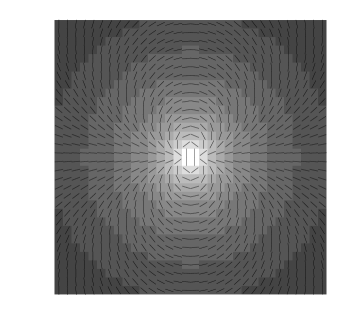
Figure 5: The $E$ and $B$ maps that result from decomposing an input map consisting of a delta function in $Q$. In this figure and the next, the lines, which are all of equal length, indicate direction. The magnitude of the polarization is indicated by the gray scale, which is logarithmic and covers a factor of $10^{4}$.

This figure illustrates the nonlocal character of the $E$/$B$ decomposition. Note that the Green functions for the potentials do not go to zero at large distances: to find the potentials, we need to specify ${\bf P}$ arbitrarily far away. Since the actual polarization is a second derivative of the potential, however, the response in the $E$ and $B$ polarization maps to a delta-function impulse does decline as the inverse square of the distance.

In the case where the map covers only part of the sky, the same approach can be used to get the pure $E$ and $B$ components of the map. However, the Green functions must be replaced by functions that satisfy the appropriate Dirichlet and Neumann boundary conditions. Such functions can in principle be found, but in practice this is unlikely to be an efficient way to perform the E/B/A separation.

A much more efficient way to perform the E/B/A separation is to split the task up into two steps:

1. Separate the map into $E$ and $B$ components without worrying about purity.

2. “Purify” each of the two maps by projecting out the ambiguous component.

The first step can be done in several ways, the most efficient being to Fourier transform the maps and do the separation mode by mode. (Equation (8) can also be used, but this will generally be slower.) If the map is of an irregular shape, it can be padded out to a convenient rectangular array in any way you like before Fourier transforming; the resulting $E$/$B$ decomposition will be correct. Different ways of doing this padding will in general lead to different decompositions, but they will differ only in where the ambiguous modes show up.

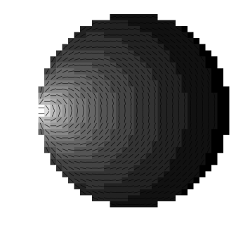
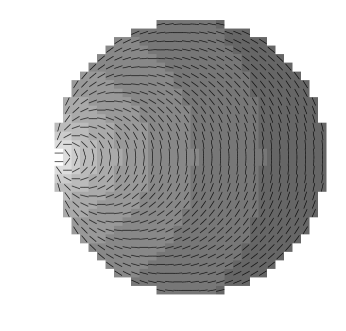
Figure 6: The $E$ and $B$ maps produced by the “ambiguous” Green functions $g_{1}$ and $g_{2}$ for a disc. As in the previous figure, the gray scale indicates the magnitude of the polarization covers a factor of $3\times 10^{5}$ logarithmically.

One way to perform the second step is to find yet more Green functions. Suppose we have an $E$ polarization map that we wish to purify. We first find a potential $\psi_{E}$ that generates this map. (This is also easily done in Fourier space.) We then subtract a biharmonic function from this potential so that the residual has the correct (Dirichlet and Neumann) boundary conditions. One way to do this is

$$\psi_{E}^{\rm pure}({\bf x})=\psi_{E}({\bf x})-\oint_{\partial\Omega}d\varphi\,[\psi_{E}(\varphi)g_{1}({\bf x};\varphi)+(\hat{\bf n}\cdot\nabla)\psi_{E}(\varphi)g_{2}({\bf x};\varphi)].$$ (10)

Here $\Omega$ represents the observed patch of sky. We use $\varphi$ to label points on the boundary $\partial\Omega$. The two Green functions $g_{1}$ and $g_{2}$ are biharmonic functions (i.e., generators of ambiguous modes) that satisfy delta-function boundary conditions. Specifically,

$$g_{1}(\varphi^{\prime};\varphi)=\delta(\varphi-\varphi^{\prime}),\qquad\qquad(\hat{\bf n}\cdot\nabla)g_{1}(\varphi^{\prime};\varphi)=0,$$ (11)

and the reverse for $g_{2}$. For the case of a disc, these Green functions can be calculated analytically and are shown in Figure 6.

The two two Green functions give the corrections that must be applied to an $E$ polarization map to purify it of any failure to meet the correct boundary conditions at any given point. (Since there are two boundary conditions, in general two corrections must be applied). Both produce polarization maps that decrease like with increasing distance: one is inversely proportional to the distance cubed, while the other is inverse square. This confirms what has been noted elsewhere [17, 18]: the ambiguous modes tend to be largest near the boundary.

In practice, equation(10) is unlikely to be the most efficient way to purify a map. Given the potential $\psi_{E}$ for an $E$ map that we wish to purify, it will generally be much faster to use other numerical methods to find a biharmonic function $\psi_{A}$ whose value and first derivative match $\psi_{E}$ on the boundary. Subtracting ${\bf D}_{E}\psi_{A}$ from the original $E$ map will purify it.

4 Conclusions

The presence of an ambiguous component in a CMB polarization map significantly affects the science that can be derived from the map. In particular, experimenters attempting to detect $B$ modes in degree-scale experiments should be sure to take $E$/$B$ confusion into account when designing experiments [16].

In a pixelized map, aliasing of small-scale power significantly worsens the problem of $E$/$B$ mixing. Especially considering the extremely blue spectrum predicted for the $E$ modes, experimenters searching for $B$ modes should be sure to heavily oversample the beam.

The E/B/A decomposition is likely to be useful in analyzing data sets. Strictly speaking, it is not necessary to perform any such decomposition: it is possible in principle to compute the likelihood function $L(C_{l}^{E},C_{l}^{B})$ for the $E$ and $B$ power spectra directly from the raw $Q$ and $U$ maps. However, decomposing the map first may increase the efficiency of the analysis, especially if we are willing to simply throw away the ambiguous modes: the likelihood function will then factor, with the each pure subspace’s contribution depending only on the corresponding power spectrum. Aside from any increase in efficiency in evaluating likelihoods, the E/B/A decomposition will be useful in checking for systematic errors and foreground contaminants and for purposes of visualization.

In [18], we presented methods for finding orthogonal bases for the E/B/A components. In many cases it may be preferable to perform the decomposition directly in map space, without finding a basis. The Green function approaches presented here are unlikely to be numerically efficient for large data sets; their primary purpose is to aid in the visualization of the E/B/A decomposition. The decomposition can be performed fairly efficiently in map space, however, in the manner briefly sketched at the end of the last section: perform an “impure” $E$/$B$ decomposition first, and then purify each component by finding a biharmonic function satisfying appropriate boundary conditions. Numerical methods for efficiently finding biharmonic functions exist.

Finally, let us note that the $E$/$B$ decomposition shows up in the analysis of weak lensing data (e.g., [20, 21]). The methods described herein may be useful in such analyses.

5 Acknowledgments

I thank Max Tegmark and Matias Zaldarriaga for many useful conversations. This work was supported by NSF grant AST-0233969. The author is a Cottrell Scholar of the Research Corporation.

References

- [1] E.M. Leitch, J.M. Kovac, C. Pryke, B. Reddall, E.S. Sandberg, M. Dragovan, J.E. Carlstrom, N.W. Halverson, & W. L. Holzapfel, Nature, 420, 763 (2002).
- [2] J.M. Kovac, E.M. Leitch, C. Pryke, J.E. Carlstrom, N.W. Halverson, & W.L. Holzapfel, Nature, 420, 772 (2002).
- [3] C.L. Bennett, M. Halpern, G. Hinshaw, N. Jarosik, A. Kogut, M. Limon, S.S. Meyer, L. Page, D.N. Spergel, G.S. Tucker, E. Wollack, E.L. Wright, C. Barnes, M.R. Greason, R.S. Hill, E. Komatsu, M.R. Nolta, N. Odegard, H.V. Peirs, L. Verde, & J. L. Weiland, astro-ph/0302207 (2003).
- [4] A. Kogut, D.N. Spergel, C. Barnes, C.L. Bennett, M. Halpern, G. Hinshaw, N. Jarosik, M. Limon, S.S. Meyer, L. Page, G. Tucker, E. Wollack, & E. L. Wright, astro-ph/0302213 (2003).
- [5] S.T. Staggs, J.O. Gundersen, & S.E. Church, in Microwave Foregrounds, edited by A. de Oliveira-Costa and M. Tegmark (ASP Conference Series, vol. 181, San Francisco), p. 299.
- [6] M.M. Hedman, D. Barkats, J.O. Gundersen, S.T. Staggs, & B. Winstein, Ap. J. Lett. 548, L111 (2001).
- [7] J.B. Peterson, J.E. Carlstrom, E.S. Cheng, M. Kamionkowski, A.E. Lange, M. Seiffert, D.N. Spergel, & A. Stebbins, astro-ph/9907276 (1999).
- [8] A. de Oliveira-Costa, M. Tegmark, M. Zaldarriaga, D. Barkats, J.O. Gundersen, M.M. Hedman, S.T. Staggs, & B. Winstein, Phys. Rev. D, 67, 023003 (2003).
- [9] http://astro.estec.esa.nl/SA-general/Projects/Planck/
- [10] M. Kamionkowski, A. Kosowsky & A. Stebbins, Phys. Rev. D 55, 7368 (1997).
- [11] M. Zaldarriaga & U. Seljak, Phys. Rev. D 55, 1830 (1997).
- [12] U. Seljak & M. Zaldarriaga, Phys. Rev. Lett. 78, 2054 (1997).
- [13] M. Kamionkowski, A. Kosowsky & A. Stebbins, Phys. Rev. Lett. 78, 2058 (1997).
- [14] A. Jaffe, M. Kamionkowski, and L. Wang, Phys. Rev. D 61, 083501 (2000).
- [15] M. Tegmark and A. de Oliveira-Costa, Phys. Rev. D 64, 063001 (2001).
- [16] E.F. Bunn, Phys. Rev. D 65, 043003 (2002).
- [17] A. Lewis, A. Challinor, and N. Turok, Phys. Rev. D 65, 023505 (2002).
- [18] E.F. Bunn, M. Zaldarriaga, M. Tegmark, & A de Oliveira-Costa, Phys. Rev. D, 67, 023501 (2003).
- [19] The map on the right is the E map.
- [20] N. Kaiser, Ap.J. 498, 26 (1998).
- [21] W. Hu & M. White, Ap.J., 554, 67 (2001).