Entropy perturbations in quartessence Chaplygin models

Abstract

We show that entropy perturbations can eliminate instabilities and oscillations, in the mass power spectrum of the quartessence Chaplygin models. Our results enlarge the current parameter space of models compatible with large scale structure and cosmic microwave background (CMB) observations.

1 Introduction

A spatially flat Universe whose evolution is driven by two components, pressureless dark matter and negative pressure dark energy, is currently considered the standard model of cosmology. In spite of its success in explaining the majority of cosmological observations, the exact nature of these components, which account for more than $90\%$ of all the matter and energy content of the Universe, is still a mystery. This situation spurred a search for alternatives and, recently, considerable work has been devoted to explore the possibility that dark matter and dark energy could be distinct manifestations, at different scales, of a single substance. This unifying dark matter-energy component is usually referred to as UDM or quartessence [1]. Two candidates for such unification, that received a lot of attention lately, are the quartessence Chaplygin fluid [2] and the quartessence tachyonic field [3].

Of course, the first and most important task is to confront the quartessence scenario with observations. In fact, it has been shown that the quartessence Chaplygin model is not much constrained by cosmological tests like SNeIa, lensing, age of the Universe etc, that involve only the background metric [4, 1, 5, 6, 7, 8]. On the other hand, tests that depend on the evolution of density perturbations, narrow the parameter space so much, that only generalized Chaplygin models whose behavior is close to the $\Lambda$CDM limit are allowed [9, 10, 11, 12]. However, in all the analyses performed so far, it is assumed that pressure perturbations are adiabatic. The main goal of this paper is to show that if intrinsic entropy perturbations are allowed the dynamics can change dramatically. A convenient choice for this quantity will make a critical length [9] in the Chaplygin component vanish and, as a consequence, instabilities and oscillations in this fluid are severely reduced. In particular we show that models with negative values for the exponent $\alpha$ of the equation of state, which are discarded by the usual analysis of adiabatic perturbations, may now be stable and, in principle, compatible with CMB and large scale structure observations.

2 Evolution of Linear Perturbations

The relativistic equations that govern the linear evolution of scalar perturbations in a multi-component fluid, in the synchronous gauge, are [13, 14]

$$\displaystyle\delta^{\prime}_{i}+3(c^{2}_{si}-w_{i})\frac{a^{\prime}}{a}\delta_{i} = -(1+w_{i})\left(kv_{i}+\frac{h^{\prime}_{L}}{2}\right)-3w_{i}\frac{a^{\prime}}{a}\Gamma_{i},$$ (2.1)

$$v^{\prime}_{i}+(1-3c^{2}_{si})\frac{a^{\prime}}{a}v_{i} = \frac{c^{2}_{si}}{1+w_{i}}k\delta_{i}+\frac{w_{i}}{1+w_{i}}k\Gamma_{i},$$ (2.2)

$$h^{\prime\prime}_{L}+\frac{a^{\prime}}{a}h^{\prime}_{L} = -\sum_{i}(1+3c^{2}_{si})8\pi G\rho_{i}a^{2}\delta_{i}-24\pi Ga^{2}\sum_{i}p_{i}\Gamma_{i},$$ (2.3)

where $\delta_{i}$, $v_{i}$, and $\Gamma_{i}$ are, respectively, the density contrast, the velocity perturbation, and the entropy perturbation of component $i$, $a$ is the scale factor, $h_{L}$ is the trace of the metric perturbation, and $k$ is the comoving wave number. For the sake of simplicity, we assume that both the spatial curvature and the anisotropic pressure perturbation vanish and that the energy-momentum tensor of each component is separately conserved. In the equations above the prime denotes derivative with respect to conformal time and, as usual, $c_{si}^{2}=p^{\prime}_{i}/\rho^{\prime}_{i}$ and $w_{i}=p_{i}/\rho_{i}$ are, respectively, the adiabatic sound speed and the equation of state parameter of component $i$.

We will consider only two components in the universe: baryons ($p_{b}=0$) and a generalized Chaplygin fluid, whose homogeneous equation of state is

$$p_{ch}=-M^{4(\alpha+1)}/\rho_{ch}^{\alpha}.$$ (2.4)

The separate conservation of the energy-momentum tensors leads to

$$\rho_{b}=\rho_{b0}a^{-3},$$ (2.5)

and

$$\rho_{ch}=\rho_{ch0}\left[(1-A)a^{-3(\alpha+1)}+A\right]^{\frac{1}{\alpha+1}},\qquad A\equiv\frac{M^{4(\alpha+1)}}{\rho_{ch0}^{\alpha+1}},$$ (2.6)

where the subscript “0” denotes quantities at the present time and we choose the scale factor today equal to unity. It then turns out that the equation of state parameter and the adiabatic sound velocity, for the Chaplygin component, are given by

$$w_{ch}(a)=-\frac{Aa^{3(\alpha+1)}}{(1-A)+Aa^{3(\alpha+1)}},$$ (2.7)

and

$$c^{2}_{sch}=-\alpha\;w_{ch}(a).\\$$ (2.8)

It is a good approximation to take $c^{2}_{sb}=0$ and we will also assume that for baryons $\Gamma_{b}=0$. When the Chaplygin component is considered, the instabilities and oscillations in the Chaplygin mass power spectrum (and, to a lesser extent, also in the baryon mass power spectrum), in the adiabatic case, have their origin in a non-vanishing value of the right-hand side in Eq. (2.2) [9]. In this case, the effective sound speed and the adiabatic sound speed are equal [15]. However, this may not be true if entropy perturbations are present [16, 17, 18]. Entropy perturbations are quite common and, since the sound speeds of baryon and the Chaplygin component are different, even for the so called “adiabatic case” there is, in fact, a relative entropy perturbation [14]. We then impose that the right-hand side of Eq. (2.2) vanishes, such that the effective sound speed for the Chaplygin component is zero. This is equivalent to assuming, as an initial condition, that $\delta p_{ch}=0$. It is straightforward to show that $\delta p_{ch}=0$ implies $d\delta{p_{ch}}/dt=0$, such that the condition is preserved [19]. With this choice we can determine the intrinsic entropy perturbation $\Gamma_{ch}$ for the Chaplygin component, obtaining

$$\Gamma_{ch}=-\frac{c^{2}_{sch}}{w_{ch}}\delta_{ch}=\alpha\;\delta_{ch}.$$ (2.9)

Since, for baryons $c_{sb}^{2}=\Gamma_{b}=w_{b}=0$, it is easy to see from Eq. (2.2), that $v_{b}$ decays rapidly and, as a matter of simplification, we take $v_{b}=0$. Also, from Eq. (2.1), we have, $\delta_{b}^{\prime}=-h_{L}^{\prime}/2$. Now, with $\Omega_{b0}+\Omega_{ch0}=1$, Eqs. (2.1)-(2.3) can be recast as

$$\frac{d\delta_{ch}}{da}-3w_{ch}(a)\frac{\delta_{ch}}{a}=-(1+w_{ch}(a))\left(\frac{kv_{ch}}{\dot{a}a}-\frac{d\delta_{b}}{da}\right),$$ (2.10)

$$\frac{dv_{ch}}{da}+(1+3\alpha w_{ch}(a))\frac{v_{ch}}{a}=0,$$ (2.11)

and

$$\frac{d^{2}\delta_{b}}{da^{2}}+\left(\frac{2}{a}+\frac{\ddot{a}}{\dot{a}^{2}}\right)\frac{d\delta_{b}}{da}=\frac{3H_{0}^{2}}{2\dot{a}^{2}}\left\{\frac{\Omega_{b0}\delta_{b}}{a^{3}}+(1-\Omega_{b0})\delta_{ch}\left[\frac{(1-A)}{a^{3(\alpha+1)}}+A\right]^{\frac{1}{\alpha+1}}\right\},$$ (2.12)

where $\dot{a}$ and $\ddot{a}$ are given by

$$\dot{a}=H_{0}\left\{\frac{\Omega_{b0}}{a}+(1-\Omega_{b0})\left[Aa^{2(\alpha+1)}+\frac{(1-A)}{a^{\alpha+1}}\right]^{\frac{1}{\alpha+1}}\right\}^{\frac{1}{2}},$$ (2.13)

$$\ddot{a}=-\frac{H_{0}^{2}}{2}\left\{\frac{\Omega_{b0}}{a^{2}}+(1-\Omega_{b0})(1+3w_{ch}(a))\left[Aa^{\alpha+1}+\frac{(1-A)}{a^{2(\alpha+1)}}\right]^{\frac{1}{\alpha+1}}\right\}.$$ (2.14)

3 Discussion

In our numerical calculations we evolved Eqs. (2.10), (2.11) and (2.12) from $z=500$ to $z=0$ to obtain the power spectra. At $z=500$ the Chaplygin fluid behaves like CDM and, to take this into account, proper initial conditions were established; we assumed $v_{ch}=0$, a scale invariant primordial spectrum and used the BBKS transfer function, [20] with the following effective shape parameter [21],[22],

$$\Gamma_{eff}=(\Omega_{b0}+(1-\Omega_{b0})(1-A)^{1/(1+\alpha)})h\;\exp\left(-\Omega_{b0}-\frac{\sqrt{2h}\;\Omega_{b0}}{\Omega_{b0}+(1-\Omega_{b0})(1-A)^{1/(1+\alpha)}}\right).$$ (3.15)

In Fig. 1 we present the Chaplygin mass power spectra, in the adiabatic case ($\Gamma_{ch}=0$), for $\alpha=-10^{-4},-10^{-5},0,10^{-5}$ and $10^{-4}$ (from top to bottom), $h=0.7$, $\Omega_{b0}=0.04$ and we choose $A$ such that all models have $\Gamma_{eff}=0.18$. The normalization of the mass power spectra is arbitrarily fixed at $k=0.01$ h Mpc^-1. For larger absolute values of $\alpha$ the oscillations and instabilities are much stronger. The data points are the power spectrum of the 2dF galaxy redshift survey as compiled in [23]. In Fig. 2, for the same parameters, we show the baryon power spectra. It is clear that, for baryons, the oscillations and, to a lesser extent, instabilities (that occur for $\alpha<0$) are quite reduced [22].

In Fig. 3 we show the mass power spectra for the Chaplygin fluid in the case $\Gamma_{ch}=\alpha\;\delta_{ch}$ ($\delta p_{ch}=0$). We considered $\alpha=-0.6,-0.3,0,0.3,0.6$ and $1$, $h=0.7$, $\Omega_{b0}=0.04$ and, again, $A$ such that all models have $\Gamma_{eff}=0.18$. The degeneracy is clear (only one curve is visually discernible) and, as remarked before, at linear scales, the oscillations and instabilities are absent. Note that models with $\alpha<0$ may now be in agreement with observations. The baryon mass power spectra curves essentially coincide with these ones. In Fig. 4 we show the mass power spectra for the Chaplygin component, in the non-adiabatic case, for the same values of $\alpha$, $h$ and $\Omega_{b0}$ as above, but now we fixed the parameter $A=0.72$, such that $\Gamma_{eff}$ is different for each model. The degeneracy has now been broken. Again the baryon mass power spectra curves are essentially identical.

In the standard cosmological model ($\Lambda$CDM and QCDM), two mysterious components, dark matter and dark energy, are predicated to explain two different phenomena: clustering of matter and cosmic acceleration. In spite of the standard cosmological model’s success, so far it has not been proven that dark matter and dark energy are, in fact, two distinct substances. A first attempt has been presented in [9]. In [12] it has been shown that CMB observations strongly constrain the parameter space of quartessence Chaplyging models, leaving little room for models dissimilar to $\Lambda$CDM. All these results are based on the assumption that there is no intrinsic entropy perturbation in the Chaplygin component. In this work we argue that if $\Gamma_{ch}=\alpha\delta_{ch}$, or, equivalently, $\delta p_{ch}=0$ as an initial condition, oscillations and instabilities, present in the adiabatic case, will disappear and, consequently, the parameter space will be enlarged (for instance, now $\alpha<0$ should be included in the analyses). We believe that the game is not over or in its final round for these models, perhaps it has just started. Anyway, our results suggest that they deserve further investigation.

Acknowledgments

We thank helpful conversations with Raul Abramo, Fabio Finelli, Martin Makler and Max Tegmark. The authors would like to thank the Brazilian research agencies CAPES, CNPq, FAPERJ and Fundação José Bonifácio for financial support.

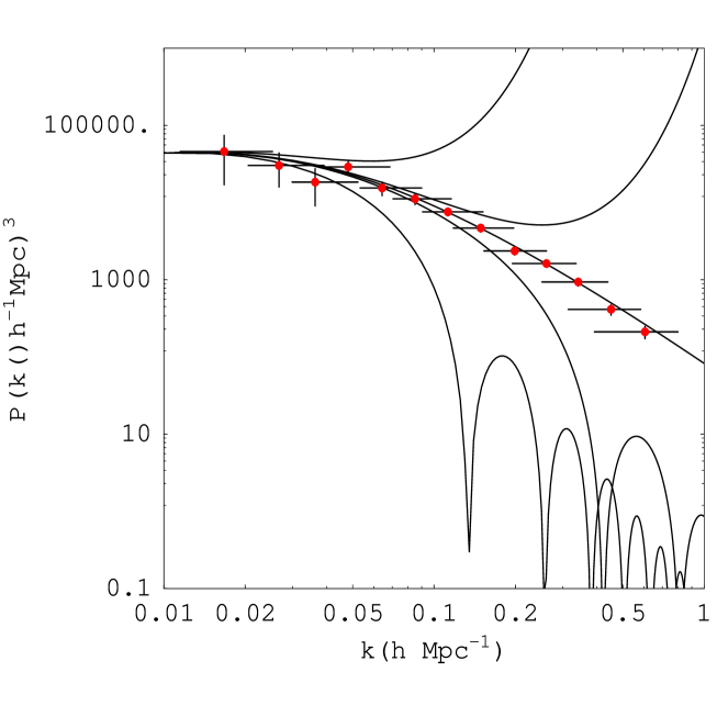
Figure 1: Chaplygin mass power spectra, in the adiabatic case, for $\alpha=-10^{-4},-10^{-5},0,10^{-5}$ and $10^{-4}$ (from top to bottom), $h=0.7$, $\Omega_{b0}=0.04$ and $A$ chosen such that all models have $\Gamma_{eff}=0.18$. The data points are the power spectrum of the 2dF galaxy redshift survey as compiled in [23].

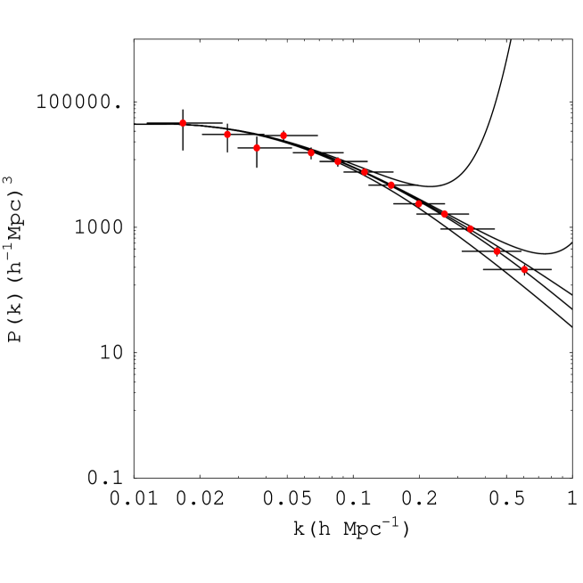
Figure 2: Baryon mass power spectra, in the adiabatic case, for $\alpha=-10^{-4},-10^{-5},0,10^{-5}$ and $10^{-4}$ (from top to bottom), $h=0.7$, $\Omega_{b0}=0.04$ and $A$ chosen such that all models have $\Gamma_{eff}=0.18$. The data points are the power spectrum of the 2dF galaxy redshift survey as compiled in [23].

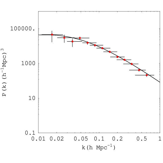
Figure 3: Chaplygin (and baryon) mass power spectra, in the non-adiabatic case, for $\alpha=-0.6,-0.3,0,0.3,0.6$ and $1$, $h=0.7$, $\Omega_{b0}=0.04$ and $A$ chosen such that all models have $\Gamma_{eff}=0.18$. The data points are the power spectrum of the 2dF galaxy redshift survey as compiled in [23].

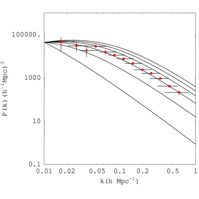
Figure 4: Chaplygin (and baryon) mass power spectra, in the non-adiabatic case, for $\alpha=-0.6,-0.3,0,0.3,0.6$ and $1$, (from bottom to top), $h=0.7$, $\Omega_{b0}=0.04$ and $A=0.72$. The data points are the power spectrum of the 2dF galaxy redshift survey as compiled in [23].

References

- [1] M. Makler, S. Q. de Oliveira, I. Waga, Phys. Lett. B 555, 1 (2003).
- [2] A. Kamenshchik, U. Moschella, V. Pasquier, Phys. Lett. B 511, 265 (2001); M. Makler, Gravitational Dynamics of Structure Formation in the Universe, PhD Thesis, Brazilian Center for Research in Physics (2001); N. Bilić, G. B. Tupper, R. D. Viollier, Phys. Lett. B 535, 17 (2002); Bento, M. C., Bertolami, O., Sen, A. A., Phys. Rev. D 66, 043507 (2002).
- [3] A. Sen, J. High Energy Phys. 04, 48 (2002); G. W. Gibbons, Phys. Lett. B 537, 1 (2002); T. Padmanabhan, T. R. Choudhury, Phys. Rev. D 66, 081301 (2002).
- [4] J. C. Fabris, S.V.B. Goncalves, P.E. de Souza, astro-ph/0207430.
- [5] P. P. Avelino, L.M.G. Beça, J. P. M. de Carvalho, C. J. A. P. Martins , P. Pinto, Phys. Rev. D 67, 023511 (2003).
- [6] R. Colistete Jr, J. C. Fabris, S.V.B. Goncalves, P.E. de Souza, astro-ph/0303338.
- [7] A. Dev, J. S. Alcaniz, D. Jain, Phys. Rev. D 67, 023515 (2003).
- [8] P. T. Silva, O. Bertolami, astro-ph/0303353.
- [9] H. Sandvik, M. Tegmark, M. Zaldarriaga, I. Waga, astro-ph/0212114.
- [10] D. Carturan, F. Finelli, astro-ph/0211626
- [11] R. Bean, O. Dore, astro-ph/0301308
- [12] L. Amendola, F. Finelli, C. Burigana, D. Carturan, astro-ph/0304325.
- [13] H. Kodama, M. Sasaki, Prog. Theor. Phys. Suppl. 78, 1 (1984).
- [14] K. A. Malik, PhD thesis, University of Portsmouth, astro-ph/0101563.
- [15] W. Hu, Astrophys. J. 506, 485 (1998).
- [16] R. R. R. Reis, Phys. Rev. D 67, 087301 (2003).
- [17] A. B. Balakin, D. Pavon, D. J. Schwarz, W. Zimdahl, to appear in New Journal of Physics, astro-ph/0302150.
- [18] U. Alam, V. Sahni, T. D. Saini, A. A. Starobinsky, astro-ph/0303009.
- [19] L. R. Abramo, F. Finelli, Phys. Rev. D 64, 083513 (2001). We thank Raul Abramo for calling our attention to this important point.
- [20] J. M. Bardeen, J. R. Bond, N. Kaiser, A. S. Szalay, Astrophys. J. 304, 15 (1986).
- [21] N. Sugiyama, Astrophys. J. Supp. 100, 281 (1995).
- [22] L. M. G. Beça, P. P. Avelino, J. P. M. de Carvalho, C. J. A. P. Martins, astro-ph/0303564.
- [23] M. Tegmark, A. J. S. Hamilton, Y. Xu, Mon. Not. R. Astron. Soc. 335, 887 (2002).