Galaxy-CMB Lensing

Abstract

A long-standing problem in astrophysics is to measure the mass associated with galaxies. Gravitational lensing provides one of the cleanest ways to make this measurement. To date, the most powerful lensing probes of galactic mass have been multiply imaged QSO’s (strong lensing of a background point source) and galaxy-galaxy lensing (weak deformation of many background galaxies). Here we point out that the mass associated with galaxies also lenses the Cosmic Microwave Background (CMB) and this effect is potentially detectable in small scale experiments. The signal is small (roughly a few tenths of $\mu$K) but has a characteristic shape and extends out well beyond the visible region of the galaxy.

I Introduction.

Flat rotation curves at large distance from galactic centers imply that the mass associated with a galaxy extends far beyond the region that is visible. Indeed, it now appears that the vast majority of the mass of a galaxy is in an unseen component, dark matter. How much dark matter is there in a galaxy and how far out does the distribution go? How does the matter associated with a single galaxy compare with the overdensity around that galaxy due to large scale structure? How is the dark matter distributed inside the galaxy? Is there substructure, as expected in simulations of Cold Dark Matter (CDM) models moore ; andrei ; bullock , or does the absence of many satellites for our Galaxy imply that the CDM models need to be modified spergel ; yoshida ; colin ; burkert ?

These questions increasingly interest not only astrophysicists studying galaxies and their properties, but also cosmologists and particle physicists, for these phenomena may depend on the power spectrum of the matter in the universe. This in turn depends on such fundamental quantities as neutrino masses and the details of inflation. If the substructure dilemma remains, the properties of dark matter, such as its scattering cross-section or annihilation rate, may be responsible. These properties may be important clues in identifying the elementary particles which constitute the dark matter and the fundamental theory governing their interactions.

The traditional method of studying the mass distribution in galaxies – measuring rotation velocities – has recently been supplemented with a relatively new technique: studying the deflection of light rays as they pass by or through the galaxy. There are a number of ways in which gravitational lensing can probe the mass distribution of an object like a galaxy, but two have emerged recently as particularly promising. First is the phenomenon of multiply imaged QSOs. Light from a background point source (the QSO) gets lensed so that multiple images are seen. The separations between these images, and more importantly their magnifications, are sensitive to the local mass distribution mao ; metcalfe ; dalal ; chiba ; keeton . Second, images of background galaxies are distorted by a foreground lensing galaxy, and the amplitude of this distortion as a function of projected distance from the center of the lens galaxy contains important information about the mass associated with that galaxy tyson ; brainerd ; fischer ; smith ; wkl ; mckay ; hoekstra ; klein . Due to the presence of large scale structure, the lensing mass extends far beyond the visible region of the galaxy. If the diameter of the visible region is of order $10$ kpc, the region within a sphere almost a thousand times larger will be overdense. Understanding this overdensity is an important step along the way to understanding galaxy formation and the correlation between mass and light in the universe berwei ; guzik ; cooray ; weidav ; bwb ; jain .

In this paper, we explore the possibility that the most distant sources of all, the Cosmic Microwave Background (CMB) anisotropies generated at redshift $z\simeq 1100$, can serve as the sources which are lensed by foreground galaxies. The problem is very similar to the lensing of the CMB by foreground galaxy clusters sz , except that the amplitude of the signal is considerably smaller here. The observed temperature $T$ as a function of 2D position $\vec{\theta}$ on the sky is

$$T(\vec{\theta}) = \tilde{T}(\vec{\theta}^{\prime})=\tilde{T}(\vec{\theta}-\vec{\delta\theta})$$ (1)

$$\simeq \tilde{T}(\vec{\theta})-\vec{\delta\theta}\cdot\nabla\tilde{T}(\vec{\theta})$$

where $\tilde{T}$ is the background CMB field originating from the unlensed position $\vec{\theta}^{\prime}=\vec{\theta}-\vec{\delta\theta}$, and $\delta\theta$ is the deflection due to the lens. As illustrated in sz , the CMB anisotropy field on small scales is almost purely a dipole (or gradient; on these small scales the two terms are interchangeable); aligning the $y-$ axis with the dipole leads to a simple expression for the observed temperature:

$$T(\vec{\theta})\simeq{\partial\tilde{T}\over\partial\theta_{y}}\times\left(\theta_{y}-\delta\theta_{y}\right).$$ (2)

Here $\partial T/\partial\theta_{y}$ is the temperature gradient, which is of course zero on average. Its rms fluctuation though is equal to $0.22\mu K$ arcsec^-1 in the standard $\Lambda$CDM cosmology with $\Omega_{\rm matter}=0.3$, $\Omega_{\rm baryon}=0.04$, $H_{0}=70$ km  sec^-1 Mpc^-1 and $\Omega_{\Lambda}=0.7$ (the rest of this paper assumes this background cosmology). The deviations from a pure dipole arise from the deflection angle $\vec{\delta\theta}$. We will see that the deflection angle induced by the mass associated with a galaxy is typically of order an arcsecond, so the expected signal is small, tenths of $\mu$K per galaxy. Eq. [2] breaks down on scales larger than ten arcminutes when the background CMB no longer behaves as a pure gradient due to the power on the scales of the acoustic peaks mc . Even on smaller scales, the “noise” due to the quadrupole can be significant as we will see in §III.

§II introduces the basic formula relating the deflection angle to the mass distribution and presents the deflection angle for several simple mass distributions. §III considers the lensing due to the large scale overdensities surrounding a galaxy. These extend out to several Mpc (or tens of arcminutes for a galaxy at redshift $0.1$). Given the resolution and sensitivity of current CMB experiments, this large scale lensing is likely to be the easiest target for future experiments. Just as in the galaxy-galaxy lensing measurements, the signal from a single foreground galaxy is quite small, so the statistics of many galaxies must be used to beat down the noise. §IV discusses the foregrounds that might contaminate this signal. We let our fancy take flight in §V where we consider the signal due to a single galaxy and show that in principle the lensed CMB can detect the sub-structure that simulations predict must exist in galactic halos. Observing this signal would require experiments with significantly better resolution and sensitivity than those currently planned, but if the small scale problems of CDM persist, we should keep this technique in mind as a way of definitively resolving the “small scale crisis.”

One final comment about previous work. Several years ago, Peiris and Spergel peiris analyzed many aspects of the CMB-galaxy cross-correlations. Their analysis, focused on the WMAP experiment wmap , and therefore is for scales larger than we consider here.

II Deflection Angle and Mass Models

The deflection angle of a photon due to a galaxy at redshift $z_{L}$, at comoving distance from us, $\chi_{L}$, is mcex

$$\vec{\delta\theta}=-8\pi G{\vec{\theta}\over\theta}\,{(\chi_{S}-\chi_{L})\over\chi_{S}}\,\left[{1+z_{L}\over\theta\chi_{L}}\int_{0}^{\chi_{L}\theta/(1+z_{L})}dR\,R~{}\Sigma(R)\right].$$ (3)

Here we take the photon to be emitted from a comoving distance $\chi_{S}=1.4\times 10^{4}$ Mpc away from us, corresponding to the surface of last scattering. Its unperturbed path has at all times an angular distance $\theta$ from the axis connecting us to the center of the galaxy. The integral is over the two dimensional mass density $\Sigma$ of the galaxy, which is assumed to be azimuthally symmetric.

A singular isothermal sphere has a density profile proportional to $r^{-2}$, so that the surface density is proportional to $R^{-1}$, where $r\,(R)$ is the 3D (2D) radius from the center of the galaxy. For this profile then the term in square brackets in Eq. [3] is independent of $\theta$ and the amplitude is fixed by the correlation length $r_{0}$ defined via

$$\rho(r)=\rho_{m}(r_{0}/r)^{2}.$$ (4)

Here $\rho_{m}$ is the average matter density in the universe, so that $8\pi G\rho_{m}=0.9H_{0}^{2}$ with $c/H_{0}=4300$ Mpc. The surface density for this distribution is $\Sigma(R)=\pi\rho_{m}r_{o}^{2}/R$, so the amplitude of the deflection angle due to a singular isothermal sphere is $0.9H_{0}^{2}\pi r_{0}^{2}=1^{\prime\prime}(r_{0}/5.6\,{\rm Mpc})^{2}$ for $\chi_{S}\gg\chi_{L}$. Simulations guzik suggest that the distribution of matter around galaxies, which is formally measured by the galaxy-mass cross-correlation function may indeed be represented by this distribution with $r_{0}\simeq 7$ Mpc. The distortion, at least on scales larger than about $100$ kpc, is therefore expected to be constant with an amplitude of a little more than an arcsecond. Figure 1 shows this deflection angle; it falls off on large scales since we do not include contributions from the density beyond $r_{0}$. Also shown is a more conservative choice of $\rho=\rho_{m}(r_{0}/r)^{-1.8}.$ Even for this choice, the expected deflection angle is of order an arcsecond.

It might seem at first that detecting such a small deflection will be hopeless given that the rms deflection of a photon from the CMB is as much as 3 arcminutes. However, this is due almost entirely to lensing by large scale (low $\ell$) fluctuations. Large patches of the CMB sky will thus be nearly uniformly deflected by up to several arcminutes, however, by $\ell=10^{4}$, the rms deflection is down to about half an arc-second. Thus, CMB lensing by galaxies will take place against a relatively smoothly-lensed background, which is still well described by a local dipole.

Figure 1: The deflection angle as a function of distance from the galactic center for several different mass models. The top two curves have an overdensity equal to $\rho_{m}\xi(r)$ with the galaxy-mass cross-correlation function equal to $(7{\rm Mpc}/r)^{\alpha}$ and $\alpha=1.8$ and $2$. The bottom curve is due to an individual halo with an NFW profile with concentration $c=8$ and maximum rotational velocity equal to $200$ km sec^-1. The galaxy is assumed to be at redshift $z_{L}=0.2$ in order to obtain the relation between angular distance (bottom axis) and physical distance (top axis).

The above estimates are for a statistical sample of galaxies, accounting for the fact that the universe is clustered, so we expect halos of dark matter to reside near each other. These estimates definitely break down on scales smaller than $\sim 100$ kpc. On these smaller scales, a more appropriate distribution is given by the Navarro, Frenk, and White (NFW) nfw profile:

$$\rho(x\equiv r/r_{s})={\rho_{s}\over x(1+x)^{2}}.$$ (5)

The NFW profile can be described by two parameters: the scale radius $r_{s}$ and the density parameter $\rho_{s}$. More commonly, these are traded in for the concentration $c$, which is the ratio of the virial radius to the scale radius, and $v_{\rm max}$, the maximum rotational velocity due to this mass distribution. The virial radius is defined as that within which the average density is equal to $\Delta\rho_{m}$ with $\Delta=337$ bryan ; bul337 for the $\Lambda$CDM model in which we are working. The maximum rotational velocity can be determined analytically in terms of $r_{s}$ and $\rho_{s}$; it is $v_{\rm max}=0.46(4\pi G\rho_{s}r_{s}^{2})^{1/2}$. Figure 1 shows the deflection due to an NFW profile with $v_{\rm max}=200$ km sec^-1 and concentration $c=8$. Analytically,

$$\delta\vec{\theta}\Big{|}_{\rm NFW}=-0.54^{\prime\prime}\,{\vec{\theta}\over\theta}\,\left({v_{\rm max}\over 200{\rm km\ sec}^{-1}}\right)^{2}{(\chi_{S}-\chi_{L})\over\chi_{S}}f(\lambda),$$ (6)

where $f(\lambda)$ is a smooth function which reaches its peak of one at $\lambda=1.3$:

$$f(\lambda)\equiv\frac{3.23}{\lambda}\cases{\ln(\lambda/2)+{\ln(\lambda/[1-\sqrt{1-\lambda^{2}}])\over\sqrt{1-\lambda^{2}}}&$\lambda<1$\cr\ln(\lambda/2)+{\pi/2-\arcsin(1/\lambda)\over\sqrt{\lambda^{2}-1}}&$\lambda>1$.}$$ (7)

$\lambda$ is defined as

$$\lambda\equiv{\chi_{L}\theta\over(1+z_{L})r_{s}}.$$ (8)

III Large Scale Galaxy-CMB Lensing

Recently, the Sloan Digital Sky Survey (SDSS) detected the signal of galaxy-galaxy lensing out to a Mpc mckay . It is useful to recap their technique to place galaxy-CMB lensing in context. They select lenses as those galaxies bright enough for spectra to have been taken (Petrosian magnitude $r^{*}<17.6$) and background galaxies fainter than $18$th magnitude. For the background galaxies, photometric redshifts are used. About $30,000$ lens galaxies are chosen from SDSS commissioning data and these are probed by about $3\times 10^{6}$ background galaxies. Thus each lens has about a hundred background galaxies behind it. The error in the shear produced by a single foreground galaxy is $0.4/\sqrt{N_{bg}}$ where the $0.4$ comes from a combination of instrumental noise and the intrinsic ellipticities of the background galaxies. Thus, if $N_{bg}=100$, the noise in the shear is $0.04$. This is almost a factor of ten larger than the expected signal. So the SDSS survey cannot detect galaxy-galaxy lensing due to a single galaxy. Instead they must average the signal over many foreground galaxies (each with a signal to noise of order $0.1$). SDSS nevertheless provides a useful measure of the galaxy-mass correlation function because there are many ($3\times 10^{4}$) foreground galaxies over which to average.

How does the SDSS signal to noise compare to that obtainable with the CMB? We have determined (Eqs. [2] and [3]) that the expected signal in a CMB experiment is

$$T(\vec{\theta})-{\partial T\over\partial\theta_{y}}\theta\cos\phi={\partial T\over\partial\theta_{y}}b(\theta)\cos\phi$$ (9)

where $\phi$ is the angle between the angular position $\vec{\theta}$ and the $y$-axis along which the background gradient is oriented and $b(\theta)$ is roughly constant with an amplitude of order one arcsecond. We also need to consider the deviation of the background anisotropy pattern $\tilde{T}$ from a pure gradient. On scales larger than $5-10^{\prime}$, the background field is more complicated. For simplicity we will assume that the background dipole can be removed but the quadrupole cannot, and it serves as a source of noise. That is, we consider the next term in the expansion of $\tilde{T}$:

$$\tilde{T}(\vec{\theta})\simeq{\partial T\over\partial\theta_{y}}\theta\cos\phi+{1\over 2}\theta_{i}\theta_{j}{\partial^{2}\tilde{T}\over\partial\theta_{i}\partial\theta_{j}}.$$ (10)

This second term on the right also has mean of zero, but variance equal to

$$\sigma_{Q}^{2}={3\over 32}\theta^{4}\sum_{l}{l^{5}C_{l}\over 2\pi}=(1.5\mu K)^{2}\left({\theta\over 1^{\prime}}\right)^{4}$$ (11)

where the second equality holds in the standard cosmology we are considering. If the quadrupole cannot be removed, then this source of noise adds in quadrature with that due to the atmosphere and/or instrument.

We can now compute the signal to noise expected for lensing of the CMB due to a single galaxy. Consider a CMB experiment which maps the sky into $N_{p}$ pixels each of area $\Delta\Omega$ with instrumental/atmospheric noise per pixel $\sigma_{n}$. Then,

$$\left({S\over N}\right)^{2} = \langle\left({\partial\tilde{T}\over\partial\theta_{y}}\right)^{2}\rangle\sum_{i}^{N_{p}}{\cos^{2}\phi_{i}\over\sigma_{n}^{2}+\sigma_{Q}^{2}(\theta_{i})}b^{2}(\theta_{i})$$ (12)

$$\simeq \langle\left({\partial\tilde{T}\over\partial\theta_{y}}b\right)^{2}\rangle\int{d^{2}\theta\over\Delta\Omega}{\cos^{2}\phi\over\sigma_{n}^{2}+\sigma_{Q}^{2}(\theta)}=\left[0.089\Big{(}{1^{\prime}\over\sqrt{\Delta\Omega}}\Big{)}\Big{(}{10\mu K\over\sigma_{n}}\Big{)}^{1/2}\right]^{2}.$$ (13)

So, for a CMB experiment to achieve resolution comparable to SDSS (signal to noise per galaxy of $0.1$), beams of order an arcminute with noise per pixel of order $10\mu$K are needed. This is within the range expected of upcoming experiments. A note of caution: the $\simeq$ sign in Eq. [13] is a warning that this signal to noise estimate assumes the pixel size is significantly smaller than the scale at which the background dipole approximation breaks down; i.e. $\Delta\Omega\ll(10^{\prime})^{2}$.

One might wonder whether, given the functional dependance of $\delta\vec{\theta}$ on the lens distance/redshift (Eq. [6] and Ref. song for example), it might not be more advantageous to look to higher redshift objects rather than SDSS galaxies as lenses For example, lyman-alpha/star-forming regions at $z\simeq 3$ might be expected to give significantly higher a $S/N$. Studying the mass distribution in such objects would indeed be of significant interest; however, since these high redshift objects will subtend a significantly smaller solid angle than medium-to-low redshift galaxies, it will have to wait until a dramatic improvement in angular resolution before their CMB-lensing signal can be properly studied. We therefore focus our attention on SDSS-type galaxies as lenses.

Since the noise from the quadrupole dominates over instrumental noise when $\theta>1^{\prime}(\sigma_{n}/1.5\mu K)^{1/2}$, and a fair fraction of the signal comes from these larger scales, reducing instrumental noise is not as a important as going to higher resolution and/or covering more sky. That is, signal to noise estimates typically scale as $(\Delta\Omega\sigma_{n}^{2})^{-1/2}$ when the dominant noise is instrumental. Here, though, the scaling is $(\Delta\Omega\sigma_{n})^{-1/2}$. For fixed resolution, then, the final signal to noise scales as $N_{rmgal}^{1/2}\sigma_{n}^{-1/2}\propto N_{p}^{1/2}\sigma_{n}^{-1/2}$. The number of pixels covered if the total time is fixed is inversely proportional to the time spent on each individual pixel, while $\sigma_{n}$ is inversely proportional to the square root of time per pixel. Therefore, the final signal to noise scales increases as less time is spent on each pixel: an experiment intent on measuring CMB-galaxy lensing should strive for large sky coverage at the expense of sensitivity.

For CMB experiments with larger beams, the approximation that the background source is a gradient breaks down. Information is still contained in the cross-correlation of the CMB and galaxy surveys peiris . As we have seen the signal is of order a tenth of a $\mu$K, while the noise per pixel due to primordial CMB fluctuations is naively of order $50\mu$K. Without a sophisticated algorithm to extract the signal, we would then need of order $500^{2}$ galaxies to beat down the noise. Going to larger redshifts to pick up these galaxies would not necessarily help since the galaxy-dark matter cross-correlation functions falls off at high redshifts, so the signal is significantly smaller. Also, a galaxy projects to a smaller angular size at high redshift, necessitating even higher resolution. Although we do not pursue it here, two possible approaches are: (i) to assume the form of the lensing profile and fit for its amplitude sz ; peiris or (ii) to extend the likelihood technique developed by Hirata and Seljak hirata to this cross-correlation case.

IV Noise

Before we assert that the lensing signal from galaxies is observable, we must identify the other potential sources of noise. Extensive discussions of CMB noise sources on small angular scales are to be found in tegmark ; toffolatti ; teho , and are reviewed in sz in the context of cluster lensing, where the issues are similar.

The expected sources of noise (other than detector noise and intrinsic noise from the CMB itself, both considered in §III) are: Galactic synchrotron, free-free and dust emission, thermal Sunyaev-Zeldovich (SZ) from galaxy clusters and filaments, kinetic SZ (including Ostriker-Vishniac) resulting from bulk gas motions, and unresolved point sources. We briefly review each of these in turn.

IV.0.1 Galactic emissions

Galactic synchrotron and free-free emission both decline with increasing $\ell$. Fluctuations due to free-free emission are already below $0.1\mu$K by $\ell=10^{4}$ above $30$ GHz teho . Above $100$ GHz synchrotron emission fluctuations are below $0.1\mu$K by $\ell=10^{3}$; at 30GHz they are predicted to be $\sim 2\mu$K at $\ell\simeq 1000$, and declining as approximately $\ell^{1/3}$ tegmark . This puts them below $1\mu$K below one arcminute. Temperature fluctuations due to Galactic dust emissions are expected to be below $1\mu$K at frequencies below 217 GHz for $\ell>3000$ if the dust emission is vibrational. The situation was less clear if the dust emission is rotational teho , but the recent WMAP wmapfor constraints suggest that rotational dust will not be a problem.

IV.0.2 Thermal SZ

Of particular interest for galaxies being observed in the foreground of an SZ cluster, are fluctuations in the cluster SZ. Clusters will themselves have substructure – component galaxies, fluctuations in electron temperature and density across the cluster. To the extent that these are resolvable, whether in the CMB data itself, in cluster radio maps, or in X-ray maps (especially with future X-ray interferometers), they could be subtracted and one could select as target galaxies those that do not have significant cluster structure in their backgrounds.

The unmodeled thermal SZ foreground has been calculated by a number of groups bond ; zhang ; hernquist . The power is proportional to $\sigma_{8}^{7}$, so there remains significant uncertainty in the amplitude. If $\sigma_{8}$ is set to its WMAP value of $0.8$ wmapspe , then the expected rms amplitude of the thermal SZ on the scales of interest is of order $5\mu$K. Of course, the signal (or in this case, the noise) goes away at $217$GHz so it is always possible in principle to avoid this source of contamination. (The relatvistic correction which spoils the null can be expected to be severely depresssed below the $5\mu$K level.)

IV.0.3 kinetic SZ and Ostriker-Vishniac

The kinetic SZ effect is the Doppler shift imprinted on CMB photons when they scatter off electrons in a moving gas. In the linear regime for the matter fluctuations this is called the Ostriker-Vishniac (OV) effect vishniac . The kinetic effect has the same spectral shape as the primordial CMB (and the lensing signal we are after) so it is more difficult to eliminate than the thermal effect. The amplitude of the effect though is of order $2\mu$K hu ; sil1 ; sil2 ; gnedin ; hernquist ; val ; ma ; zhang ; zh2 , so it is not a major stumbling block.

IV.0.4 Point Sources

Toffolatti et. al. toffolatti considered the contribution of unresolved point sources to fluctuations in the anisotropy of the CMB on 1-100 arcminute scales, at the 8 Planck wavebands from 30GHz to 857GHz. These sources include, in the low frequency channels, radio loud AGNs, flat-spectrum radio-galaxies, quasars, and high-z BL-Lacs. Dust emission from distant dust-rich young galaxies is the dominant source at higher frequencies. Assuming that point sources with flux below 1mJy remain unsubtracted, they find (figures 5 and 6) that in all channels $\langle(\Delta T/T)^{2}\rangle^{1/2}>10^{-6}$ at 1 arcminute (best channel – 143 GHz), and in many cases is much bigger. It is also increasing with decreasing $\theta$ as approximately $\theta^{-1}$, suggesting that in the best channels (between about 44 and 150 GHz) we can expect point sources to contribute about 5-10 microK of noise at 6 arcsecond , and maybe 10-15 microK of noise at 1 arcsecond.

To make much improvement in these noise figures you would need to be able to accurately subtract very low flux point sources – about 0.1 mJy to achieve a a factor of 3, 0.01mJy to get down an order of magnitude. It is also true that point sources will not exhibit the coherent extended structure expected from lensing and may possibly be filtered out. The biggest confusion is likely to arise if we attempt to use galaxy lensing to measure the proto-galactic substructures. On this scale the foreground dust emission is dominant. However, it also has a rather different energy spectrum than the SZ-distorted CMB, which may aid in its subtraction.

IV.0.5 Other Sources of Confusion

There are several other effects that produce signals similar to that considered here. Moving clusters produce nonlinear corrections to the Integrated Sachs Wolfe Effect on small scales, and the pattern produced has the same structure as that due to lensing. The signal is quite small thoughaghanim ; coo2 ($\sim 0.3\mu$K) and on larger scales than interest us. Coherent electron rotational velocities in clusters lead to a dipolar signaturecooche ; chluba and these are on relatively small scales. But the amplitude is also very small and the induced signal is not aligned with the cosmic dipole.

V Single Galaxy Lensing

The lensing signal due to the halo surrounding a single galaxy is given by Eq. [6]. Since the signal is very small, we cannot hope to measure it with the current, or even currently planned, CMB experiments. Here we simply motivate future experiments by illustrating that the potential pay-off is large: lensing of the CMB in principle allows us to differentiate between an NFW profile and an isothermal profile, thereby testing one result of numerical simulations. More ambitiously, very high resolution measurements could detect the sub-structure predicted by current theories of structure formation.

Detecting the shape of the dark matter profile around a single galaxy with CMB lensing requires resolution and sensitivity far beyond current capabilities. Figure 2 shows the different signals induced by an NFW profile and an isothermal profile. The galaxy is situated at $z=0.1$ (the lower the redshift, the larger it appears, and therefore the less difficult is the issue of resolution). A number of groups bul337 have found that typical values of the concentration parameter of galaxies at redshift one are $5-10$ in CDM models. The galaxy doing the lensing in Figure 2 has concentration parameter equal to eight and a maximum circular velocity of $200$ km sec^-1. This corresponds to a scale radius $r_{s}=44$ kpc and a virial mass of $2\times 10^{12}h^{-1}M_{\odot}$.

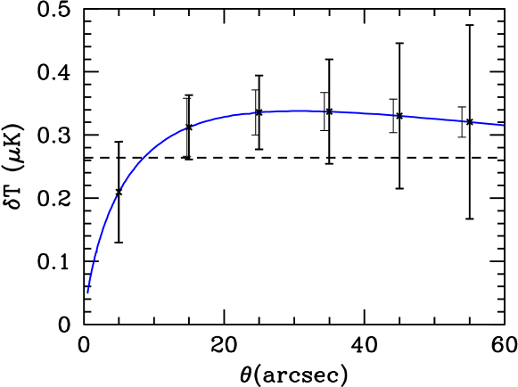
Figure 2: Anisotropy induced by lensing by an NFW dark matter profile (solid curve) and an isothermal sphere (dashed straight line), with the galaxy sitting at redshift $0.1$. The galaxy is chosen to have concentration $8$ and scale radius equal to $44$ kpc (corresponding to maximum rotational velocity of order $200$ km sec^-1). Errors are shown for a $5^{\prime\prime}$ beam with $0.4\mu$K instrumental noise per pixel. Light error bars do not include noise from the background quadrupole; larger, heavier bars do.

Even Figure 2, with its optimistic noise and resolution parameters, paints too pretty a picture. For, we have neglected all foregrounds, save for the local quadrupole of the CMB. Noise due to the quadrupole kicks in at surprisingly small scales, because of the exquisite sensitivity required to discriminate these models.

The surface density of a smooth NFW profile with these parameters is depicted in Figure 3. Unhindered by experimental complications, we are led to ask whether a smooth NFW profile could be distinguished from the clumpy profiles found in simulations.

 

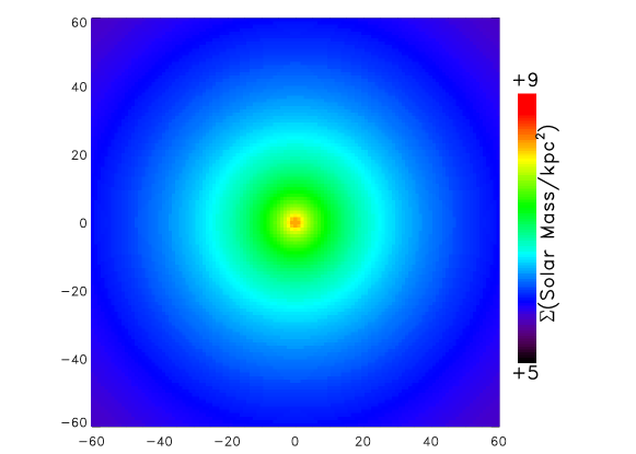
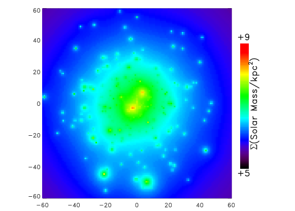
Figure 3: Log of the surface density of a galaxy at redshift one. Axes are in units of arcsec. Left Panel: NFW profile with a scale radius equal to $44$ km and a maximum circular velocity of $200$ km sec ^-1. Right Panel: The same mass distributed in $240$ sub-halos.

To construct a clumpy halo, we use the distribution of sub-halos measured by moore . They find that the cumulative number of halos with circular velocity greater than $v_{\rm max}$ is roughly equal to $0.03(v_{\rm max}/v_{\rm parent})^{-3}$. This means that the distribution of halos

$$dn/dv_{\rm max}\simeq\cases{0.09\left({v_{\rm parent}^{3}\over v_{\rm max}^{4}}\right)&$v_{\rm max}>v_{\rm cutoff}$\cr 0&otherwise}.$$ (14)

Here the lower cut-off arises because we don’t know what the simulations predict on such small scales. Note that with this distribution, if we take $v_{\rm cutoff}=0.05v_{\rm parent}$, there are $240$ sub-halos in the galaxy.

To generate a distribution of velocities of sub-halos, first normalize Eq. [14] to unity: $dn^{\rm norm}/dv_{\rm max}=(1/N)dn/dv_{\rm max}$ and then given a random number $\eta$ between zero and one, define the velocity of one sub-halo $v$ via

$$\eta=\int_{v_{\rm cutoff}}^{v}dv_{\rm max}{dn^{\rm norm}\over dv_{\rm max}}.$$ (15)

In this case we can do the integral analytically, so

$$v_{\rm max}={v_{\rm cutoff}\over(1-\eta)^{1/3}}.$$ (16)

We can use the same technique to generate the spatial distribution of halos. Suppose that the number of halos is distributed according to an NFW profile. We want $\Sigma(R)$ from the sub-structure to follow an NFW profile. The total mass within a radius $R$ is $2\pi\int_{0}^{R}dR^{\prime}\,R^{\prime}\,\Sigma_{\rm NFW}(R^{\prime})$. So the fraction of the total mass which is within $R$ is

$$\eta(R)={\int_{0}^{R/r_{s}}dx\,x\,\Sigma_{\rm NFW}(x)\over\int_{0}^{R_{max}/r_{s}}dx\,x\,\Sigma_{\rm NFW}(x)}.$$ (17)

Here we have cut off the distribution at $R_{\rm max}=10r_{s}$; note that $\eta$ lies between zero and one, so a random number between zero and one can be associated with a given value of $R$. The angular coordinate of the sub-halo is also assigned randomly. This distribution is shown in the right panel of Figure 3.

 

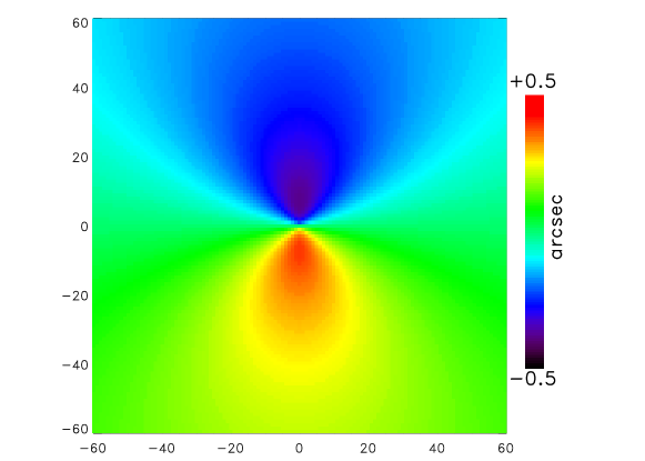
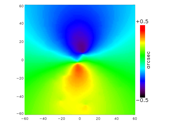
Figure 4: Temperature profile due to lensing of the background CMB by a foreground galaxy at redshift one. The background CMB is a pure dipole aligned from bottom to top. Left Panel: Lensing due to smooth galaxy depicted in left panel of Figure 3. Right Panel: Lensing due to the clumpy galaxy shown in right panel of Figure 3.

Figure 4 shows the imprint on the CMB resulting from both the smooth and the clumpy galaxy. Note the characteristic signal first pointed out in Ref. sz : a hot and cold lobe on either side of the galactic center. (Here we have subtracted off the dipole.) Traces of the substructure are still evident in the right panel of Figure 4. However, these are much less obvious than those in the surface density plot of Figure 3. The similarity of the two panels in Figure 4 is reflection of the fact that the galaxy is lensing a large “sheet,” the background dipole, as opposed to the point-like QSO’s with which we are more familiar pkeet .

 

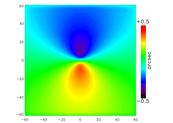
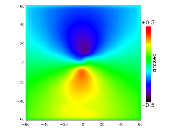
Figure 5: The signals shown in Figure 4 smoothed with a $5$ arcsec beam.

A realistic CMB experiment will have a finite width beam. Figure 5 shows the results of smoothing the signal with a beam of full width half maximum of $5^{\prime\prime}$. Even after such smoothing, there remains a noticeable difference between the clumpy and smooth galaxies.

VI Conclusion

Mass surrounding a galaxy lenses the background cosmic photons arriving from the surface of last scattering at $z\simeq 1100$. This lensing can be used to probe the dark matter distribution around galaxies. On the relevant scales – of order an arcminute – the background is nearly a dipole, and the amplitude of the signal is of order $1^{\prime\prime}\times\partial T/\partial\theta\sim 0.2\mu$K. This signal can be used in two fundamentally different ways. On the one hand, one can average over many foreground galaxies so as to obtain a measure of the galaxy-mass correlation function. We have shown that given enough sky coverage a CMB experiment with an arcminute beam size and noise of $10\mu$K per pixel would be able to make a measurement of this correlation function that is competitive with SDSS. Instruments like the Penn Bolometric Array – a $3$mm camera for the $100$m Green Bank telescope – hold some promise for beginning a more detailed exploration of galaxy mass distributions. It is worth noting that, unlike measurements of lensing-induced shear or amplification, which are sensitive to the second derivative of the lens gravitational potential, $\Phi$, this proposed measurement of the deflection angle is sensitive to $\nabla\Phi$. In principle, the inversion to obtain $\Phi$, is far easier from $\nabla\Phi$ than from $\nabla\nabla\Phi$.”

In the distant future, we might be able to go further and probe the dark matter halo of an individual galaxy. For noise levels reached today, the signal to noise from a single galaxy is of order $1/100$. Either noise levels will have to come down appreciably, or a different source needs to be used. This latter option is intriguing. One particularly appealing possibility is to use the gradient caused by the thermal Sunyaev-Zel’dovich (SZ) effect (the scattering of CMB photons by electrons in an ionized plasma) from a background galaxy cluster. This results from CMB photons scattering off hot electrons in the cluster’s ionized IGM. A typical expected temperature gradient is of order $500\mu$K arcmin^-1, almost two orders of magnitude above that from the primordial CMB. If a galaxy were positioned along the line of sight to a cluster, where the SZ effect would look nearly like a gradient on sub-arcminute scales, then we would expect the galaxy lensing signal to be $\sim 5-10\mu$K. This is then comparable to current noise levels in CMB experiments, so might be the best hope of measuring this fascinating signal in the near future.

The work of SD is supported by the DOE, by NASA grant NAG5-10842, and by NSF Grant PHY-0079251. GDS is supported by a DOE grant to astrophysics theory group at CWRU. GDS thanks the astrophysics group at Fermilab where this work began and the Kavli Institute for Theoretical Physics where much of this work was completed. The Kavli Institute is supported in part by National Science Foundation grant PHY99-07949. We thank Asantha Cooray and Andrey Kravstov for very helpful comments on an earlier draft and Lam Hui and Charles Keeton for their insight and advice.

References

- (1) B. Moore et al., Astrophys. J. 524, L19 (1999)
- (2) A. Klypin, A. V. Kravtsov, O. Valenzuela, and F. Prada, Astrophys. J. 522, 82 (1999)
- (3) J. S. Bullock, A. V. Kravtsov, and D. H. Weinberg, Astrophys. J. 539, 517 (2000)
- (4) D. N. Spergel and P. J. Steinhardt, Phys. Rev. Letters 84, 3760 (2000)
- (5) N. Yoshida, V. Springel, S. D. M. White, and G. Tormen, Astrophys. J. 544, L87 (2000)
- (6) P. Colin, V. Avila-Reese, O. Valenzuela, and C. Firmiani, Astrophys. J. 581, 777 (2002)
- (7) E. D’Onghia and A. Burkert, Astrophys. J. 586, 12 (2003)
- (8) S. Mao and P. Schneider, Monthly Notices of Royal Astronomical Society 295, 587 (1998)
- (9) R. B. Metcalfe and P. Madau, Astrophys. J. 563, 9 (2001)
- (10) N. Dalal and C. S. Kochanek, Astrophys. J. 572, 25 (2002)
- (11) M. Chiba, Astrophys. J. 565, 17 (2002)
- (12) C. Keeton, astro-ph/0111595
- (13) J. A. Tyson, F. Valdes, J. F. Jarvis, and A. P. Mills, Astrophys. J. 281, L59 (1984)
- (14) T. G. Brainerd, R. D. Blanford, and I. Smail, Astrophys. J. 466, 623 (1996)
- (15) P. Fischer et al., Astronomical J. 120, 1198 (2000)
- (16) D. Smith, G. Bernstein, P. Fischer, and M. Jarvis, Astrophys. J. 551, 643 (2000)
- (17) G. Wilson, N. Kaiser, G. A. Luppino, and L. L. Cowie, Astrophys. J. 555, 572 (2001)
- (18) T. A. McKay et al., astro-ph/0108013
- (19) Y.-S. Song, A. Cooray, L. Knox, and M. Zaldarriaga, astro-ph/0209001
- (20) H. Hoekstra et al., astro-ph/0206103
- (21) M. Kleinheinrich et al., astro-ph/0304208
- (22) A. A. Berlind and D. H. Weinberg, Astrophys. J. 575, 587 (2002)
- (23) J. Guzik and U. Seljak, Monthly Notices of Royal Astronomical Society 321, 439 (2001)
- (24) A. Cooray, astro-ph/0206068
- (25) D. H. Weinberg, R. Dav’e, N. Katz, and L. Hernquist, astro-ph/0212356
- (26) A. A. Berlind et al., astro-ph/0212357
- (27) B. Jain, R. Scranton, and R K. Sheth, astro-ph/0304203
- (28) U. Seljak and M. Zaldarriaga, Astrophys. J. 538, 57 (2000)
- (29) S. Dodelson, Modern Cosmology (Academic Press, Amsterdam, 2003)
- (30) H. V. Peiris and D. N. Spergel, Astrophys. J. 540, 605 (2000)
- (31) C. L. Bennett et al., astro-ph/0302207
- (32) See, e.g., J. A. Peacock, Cosmological Physics (Cambridge University Press, Cambridge, 1999) or Ref. mc , Chapter 10.
- (33) J. F. Navarro, C. S. Frenk, and S. D. M. White, Astrophys. J. 462, 563 (1996)
- (34) G. Bryan and M. Norman, Astrophys. J. 495, 80 (1998)
- (35) J. Bullock et al., Monthly Notices of Royal Astronomical Society 321, 559 (2001)
- (36) C. Hirata and U. Seljak, Phys. Rev. D 67, 043001 (2003)
- (37) M. Tegmark and G. Efstathiou, Monthly Notices of Royal Astronomical Society 281, 1297 (1996)
- (38) M. Toffolatti et al., Monthly Notices of Royal Astronomical Society 297, 117 (1998)
- (39) M. Tegmark, D. J. Eisenstein, W. Hu, and A. de Oliveira-Costa, Astrophys. J. 530, 133 (2000)
- (40) C. L. Bennett et al., astro-ph/0302208
- (41) P. J. Zhang, U.-L. Pen, and B. Wang, Astrophys. J. 577, 555 (2002)
- (42) J. R. Bond, M. I. Ruetalo, J. W. Wadsley, and M. D. Gladders, astro-ph/0112499
- (43) V. Springel, M. White, and L. Hernquist, Astrophys. J. 549, 681 (2001) ; M. White, L. Hernquist, and V. Springel, Astrophys. J. 579, 16 (2002)
- (44) D. N. Spergel et al., astro-ph/0302209
- (45) J. P. Ostriker and E. Vishniac, Astrophys. J. 306, 51 (1986) ; E. Vishniac, Astrophys. J. 322, 597 (1987)
- (46) W. Hu, Astrophys. J. 529, 12 (2000)
- (47) A. C. da Silva, et al. Monthly Notices of Royal Astronomical Society 326, 155 (2001)
- (48) A. C. da Silva, et al., Astrophys. J. 561, L15 (2001)
- (49) N. Y. Gnedin and A. Jaffe, Astrophys. J. 551, 3 (2001)
- (50) P. Valageas, A. Balbi, and J. Silk, Astronom and Astrophys. 367, 1 (2001)
- (51) C.-P. Ma and J. N. Fry, Phys. Rev. Letters 88, 211301 (2002)
- (52) P. Zhang, U-L. Pen, and H. Trac, astro-ph/0304534
- (53) N. Aghanim, S. Prunet, O. Forni, and F. R. Bouchet, Astronom and Astrophys. 334, 409 (1998)
- (54) A. Cooray, Phys. Rev. D 65, 083518 (2002)
- (55) A. Cooray and X. Chen, Astrophys. J. 573, 43 (2002)
- (56) J. Chluba and K. Mannheim, astro-ph/0208392
- (57) C. Keeton, private communication