Measurement of the gravitational potential evolution from the cross-correlation between WMAP and the APM Galaxy survey

Abstract

Models with late time cosmic acceleration, such as the $\Lambda$-dominated CDM model, predict a freeze out for the growth of linear gravitational potential at moderate redshift $z<1$, what can be observed as temperature anisotropies in the CMB: the so called integrated Sachs-Wolfe (ISW) effect. We present a direct measurement of the ISW effect based on the angular cross-correlation function, $w_{TG}(\theta)$, of CMB temperature anisotropies and dark-matter fluctuations traced by galaxies. We cross-correlate the first-year WMAP data in combination with the APM Galaxy survey. On the largest scales, $\theta=4-10$ deg, we detect a non-vanishing cross-correlation at 98.8% significance level, with a 1-$\sigma$ error of $w_{TG}=0.35\pm 0.14\mu$K, what favors large values of $\Omega_{\Lambda}\simeq 0.8$ for flat FRW models. On smaller scales, $\theta<1$deg, the correlations disappear. This is contrary to what would be expected from the ISW effect, but the absence of correlations may be simply explained if the ISW signal was being cancelled by anti-correlations arising from the thermal Sunyaev-Zeldovich (SZ) effect.

1 Introduction

The recent measurements of CMB anisotropies made public by the WMAP team are in good agreement with a ‘concordance’ cosmology based on the $\Lambda$CDM model. The unprecedented sensitivity, frequency and sky coverage of this new data set provides us the opportunity of asking new questions about the evolution of the universe. In this paper we present the cross-correlation of the cosmic microwave background (CMB) anisotropies measured by WMAP (?), with galaxies in the APM Galaxy Survey (?). In the observationally favored $\Lambda$CDM models, a non-vanishing CMB-galaxy cross-correlation signal arises from the distortion of the pattern of primary CMB anisotropies by the large-scale structures as microwave photons travel from the last scattering surface to us. On large angular scales such distortion is mainly produced by the energy injection photons experience as they cross time-evolving dark-matter gravitational potential wells: the so-called integrated Sachs-Wolfe effect (?). On smaller scales additional secondary anisotropies are produced when photons scatter off hot intra-cluster gas, ie the Sunyaev-Zeldovich effect (?).

In this work, we shall use optical galaxies from the APM survey as tracers of the large-scale dark-matter distribution of the universe. The APM Survey has produced one of the best estimates of the angular galaxy 2-point correlation function to date. Its shape on large scales led to the discovery of excess large-scale power, and gave early indications of the $\Lambda$CDM model (?; ?; ?), (?). Higher-order correlations have also been studied in the APM Galaxy Survey (?; ?; ?). For the first time, these measurements were accurate enough and extended to sufficiently large scales to probe the weakly non-linear regime with a reliable Survey. The results are in good agreement with gravitational growth for a model with initial Gaussian fluctuations. They also indicate that the APM galaxies are relatively unbiased tracers of the mass on large scales (?). Moreover the APM results are in excellent agreement with other wide field photometric surveys, such as the Sloan Digital Sky Survey (SDSS), for both number counts and clustering (?; ?; ?; ?).

2 Data & simulations

The APM Galaxy Survey (?) is based on 185 UK IIIA-J Schmidt photographic plates each corresponding to $5.8\times 5.8$ deg² on the sky limited to $b_{J}\simeq 20.5$ and having a mean depth of $\simeq 400$ Mpc/h for $b<-40$ deg and $\delta<-20$ deg. These fields were scanned by the APM machine and carefully matched using the $5.8\times 0.8$ deg² plate overlaps. Out of the APM Survey we considered a $17<b_{J}<20$ magnitude slice, which includes 1.2 million galaxies at a mean redshift $\bar{z}=0.15$, in an equal-area projection pixel map with a resolution of $3.5^{\prime}$, that covers over $4300$ deg² around the SGC.

We use the full-sky CMB maps from the first-year WMAP data (?). In particular, we have chosen the V-band ($\sim 61$ GHz) for our analysis since it has a lower pixel noise than the highest frequency W-band ($\sim 94$ GHz), while it has sufficiently high spatial resolution ($21^{\prime}$) to map the typical Abell cluster radius at the mean APM depth. We mask out pixels using Kp0 mask, which cuts $21.4\%$ of sky pixels (?), to make sure Galactic emission does not affect our analysis. WMAP and APM data are digitized into $7^{\prime}$ pixels using the HEALPix tessellation . Figs 1 show these maps smoothed using a Gaussian beam of FWHM $=5$ deg (left) and $0.7$ deg (right panels).

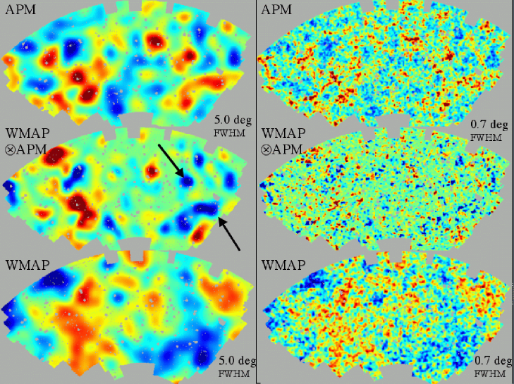
Figure 1: APM galaxy density fluctuation maps (top panels) compared to WMAP (V-band) maps (bottom panels) and the cross-correlation map (middle). In each case left panels show the maps smoothed with a Gaussian beam of FWHM $=5$ deg, while right panels have FWHM $=0.7$ deg. We use normalized units (dimensionless) with linear color scheme in the range ($-3\sigma,+3\sigma$), being $\sigma$ the pixel variance in each map.

To determine the accuracy of our error estimation we run $200$ WMAP V-band Monte-Carlo realizations. We simulate the signal by making random realizations of the CMB angular power-spectrum as measured by WMAP, convolved with its measured symmetrized beam profile, to which we add random realizations of the white noise estimated for the V-band (?). Sampling variance in the WMAP-APM cross-correlation is thus evaluated by computing the correlation between the simulated V-band CMB maps (with WMAP Kp0 mask pixels removed) and the APM survey.

3 WMAP-APM Cross-Correlation

We define the cross-correlation function as the expectation value of density fluctuations $\delta_{G}=N_{G}/<N_{G}>-1$ and temperature anisotropies $\Delta_{T}=T-T_{0}$ (in $\mu$K) at two positions ${\hat{n}}_{1}$ and ${\hat{n}}_{2}$ in the sky: $w_{TG}(\theta)\equiv\langle\Delta_{T}({\bf{\hat{n}}_{1}})\delta_{G}({\bf{\hat{n}}_{2}})\rangle$, where $\theta=|\bf{{\hat{n}}_{2}}-\bf{{\hat{n}}_{1}}|$, assuming that the distribution is statistically isotropic. To estimate $w_{TG}(\theta)$ from the pixel maps we use:

$$\mbox{$$}w_{TG}(\theta)={\sum_{i,j}\Delta_{T}({\bf{\hat{n}}_{i}})~{}\delta_{G}({\bf{\hat{n}}_{j}})~{}w_{i}~{}w_{j}\over{\sum_{i,j}w_{i}~{}w_{j}}},$$ (1)

where the sum extends to all pairs $i,j$ separated by $\theta\pm\Delta\theta$. The mean temperature fluctuation is subtracted $\langle\Delta_{T}\rangle=0$. The weights $w_{i}$ can be used to minimize the variance when the pixel noise is not uniform, however this introduces larger cosmic variance. Here we follow the WMAP team and use uniform weights (i.e. $w_{i}=1$). We consider angular scales, $\theta<10$ deg. Cross-correlations are expected to be dominated by sampling variance beyond $\sim 10$ deg, where the APM angular correlation function vanishes. Fig 2 shows the resulting cross-correlation. On scales above $\theta>5$ deg there is a significant correlation above the estimated error-bars.

Fig 2 shows the 1-$\sigma$ confidence interval for $w_{TG}(\theta)$ obtained using the jack-knife covariance matrix. Surveys are first divided into $M=10$ (similar results are found for $M=10-20$) separate regions on the sky, each of equal area. The analysis is then performed $M$ times, each time removing a different region, the so-called jack-knife subsamples, which we label $k=1\dots M$. The estimated statistical covariance for $w_{TG}$ at scales $\theta_{i}$ and $\theta_{j}$ is then given by:

$$\mbox{$$}C_{ij}={M-1\over{M}}\sum_{k=1}^{M}\Delta w_{TG}^{k}(\theta_{i})\Delta w_{TG}^{k}(\theta_{j})$$ (2)

where $\Delta w_{TG}^{k}(\theta_{i})$ is the difference between the $k$-th subsample and the mean value for the $M$ subsamples. The case $i=j$ gives the error variance. The accuracy of the jack-knife covariance have been tested for both WMAP (?) and the APM and SDSS survey (?; ?; ?; ?).

We have used the Monte-Carlo (MC) simulations described above to find that the jack-knife (JK) errors from a single MC simulation agree very well (better than $20\%$ accuracy), with the MC error from 200 realizations. This is shown in Fig. 3. The JK error from a single realization (shown as squares) is in excellent agreement with the MC error (dispersion from 200 realizations, shown as continuous line). Thus, in our case, using JK errors over a single realization gives an unbiased estimation of the true error, but the variance (shown as errorbars in Fig. 3) in this error estimation can be as large as $20\%$.

On the other hand, the JK errors in the real WMAP-APM sample are shown as a dashed line in Fig. 3. They are comparable to the errors we measure using the MC simulations on scales $\theta>4$ deg, where the JK errors are potentially subject to larger biases (as we approach the size of the JK subsample). On smaller scales, the JK errors from WMAP are up to a factor 2 smaller than the JK errors (or sample to sample dispersion) within the MC simulations. The deviation is significant, given the errorbars, and it therefore shows that the MC simulations (rather than the JK error method) fail to reproduce the WMAP-APM data on small scales. This is not very surprising as the MC simulations do not include any physical correlation that might be present in WMAP-APM and assume a CMB power spectrum that is valid for the whole sky, and not constraint to reproduce the WMAP power over the APM region. Alternatively, the JK errors provide a model free estimation that is only subject to moderate ($20\%$) uncertainty, while MC errors depend crucially on the model assumptions used to produce simulations.

Despite these differences in the errors on small scales, the overall significance for the detection on different scales is similar when we use the $\chi^{2}$ values below or when we ask how many of the 200 MC simulations have a signal and JK error comparable to the observations. When a particular MC simulation has an accidentally large cross-correlation signal, it also has a large noise (JK error) associated. We find that at 5 degrees only one of MC simulations have a signal to noise ratio comparable to the observed WMAP-APM correlation on large scales. This means that the significance of the cross-correlation detection is better than $1\%$. We can now estimate confidence regions in $w_{TG}$ using a $\chi^{2}$ test with the JK covariance matrix:

$$\mbox{$$}\chi^{2}=\sum_{i,j=1}^{N}\Delta_{i}~{}C_{ij}^{-1}~{}\Delta_{j},$$ (3)

where $\Delta_{i}\equiv w_{TG}^{E}(\theta_{i})-w_{TG}^{M}(\theta_{i})$ is the difference between the ”estimation” $E$ and the model $M$. The $\chi^{2}$ test gives a best fit constant $w_{TG}=0.35\pm 0.13\mu$K (the error corresponds to 68% C.L. $\chi^{2}_{min}=0.19$) for the 3 bins in the range $\theta=4-10$ degrees. For this range of scales, a constant null correlation $w_{TG}=0$ gives $\Delta\chi^{2}=6.1$ which has a probability of $P=1.2\%$ and sets the significance of our detection to $2.5\sigma$. We find similar results when we use the MC covariance matrix (eg, $\chi^{2}_{min}=0.33$ for best fit; $\Delta\chi=5.3$ and $P=2\%$ for the significance of the detection) but concentrate on the JK matrix from now on for the reasons given above.

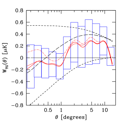
Figure 2: Comparing measurement to predictions: The two solid lines and the dotted line show $w_{TG}$ results for WMAP bands V, W, and the foreground “cleaned” map. Boxes give the $68\%$ confidence levels. Also shown are the theoretical predictions for ISW and SZ (upper and lower short-dashed lines) and their sum (long-dashed line) for the best-fit model with $\Omega_{\Lambda}\simeq 0.8$.

Figure 3: Errors in the cross-correlation $w_{TG}(\theta)$ from the dispersion in 200 Monte-Carlo simulations (solid line) as compared with the mean and dispersion (squares with errobars) in the jack-knife error estimation over the same simulations. Dashed line correspond to the jack-knife error in the real WMAP-APM sample.

3.1 Comparison with Predictions

Galaxy fluctuations in the sky can be modeled as, $\delta_{G}({\hat{n}})=\int dz~{}\phi_{G}(z)~{}\delta_{G}({\hat{n}},z)$ where $\phi_{G}(z)$ models the survey selection function along the line-of-sight. We will assume here that APM galaxies are good tracers of the mass on large scales (see §1), so that we can use the linear bias relation: $\delta_{G}\simeq b\delta$, with $b\simeq 1$ and for the power spectrum: $P_{G}(k,z)\simeq b(z)^{2}P(k,z)$. In the linear regime we further have: $P(k,z)=D^{2}(z)~{}P(k)$. We can then define a galaxy window function $W_{G}(z)\simeq b(z)~{}D(z)~{}\phi_{G}(z)$ accounting for bias, linear growth, and the galaxy selection function. For the APM selection we use the function in (?) with a mean redshift $\bar{z}\simeq 0.15$. Thus the galaxy 2-point angular correlation is (?),(?) $w_{GG}(\theta)=<\delta_{G}\delta_{G}>=\int dk~{}k~{}P(k)~{}g_{G}(k\theta)$, where the kernel $g_{G}(k\,\theta)$ is a line-of-sight integral, $g_{G}(k\theta)={1/{2\pi}}~{}\int dz~{}W_{G}^{2}(z)~{}j_{0}(k\theta\,r)$ where $j_{0}$ is the zero-th order Bessel function, and $r(z)$ denotes comoving distance. We use (?) for the linear power spectrum, with shape parameter $\Gamma=\Omega_{m}h$, and $h=0.7$. We take $\sigma_{8}=1$ and $b=1$ which give a resonable match to the measured variance in the APM (?).

The temperature of CMB photons is gravitationally blueshifted as they travel through the time-evolving dark-matter gravitational potential wells along the line-of-sight, from the last scattering surface $z_{s}=1089$ to us today, $z=0$ (?). At a given sky position ${\bf{\hat{n}}}$: $\Delta T^{ISW}({\bf{\hat{n}}})=-2\int~{}dz~{}\dot{\Phi}({\bf{\hat{n}}},z)$. For a flat universe $\nabla^{2}\Phi=-4\pi Ga^{2}\rho_{m}\delta$ (?), which in Fourier space reads, $\Phi(k,z)=-3/2\Omega_{m}~{}(H_{0}/k)^{2}~{}\delta(k,z)/a$. Thus:

$$\mbox{$$}w_{TG}^{ISW}(\theta) = <\Delta_{T}^{ISW}\delta_{G}>=\int{dk\over k}~{}P(k)~{}g(k\theta)$$ (4)

$$g(k\theta) = {1\over{2\pi}}~{}\int dz~{}W_{ISW}(z)~{}W_{G}(z)~{}j_{0}(k\theta\,r)$$

where the ISW window function is given by $W_{ISW}=-3~{}\Omega_{m}~{}({H_{0}\over c})^{2}~{}\dot{F}(z)$, with $c/H_{0}\simeq 3000h$ Mpc^-1 the Hubble radius today. $\dot{F}=d(D/a)/dr=(H/c)D(f-1)$ with $f\simeq\Omega_{m}^{6/11}(z)$ quantifies the time evolution of the gravitational potential. Note that $\dot{F}$ decreases as a function of increasing redshift (as $\Omega_{m}(z)\rightarrow 1$). It turns out that for flat universes, $\Omega_{m}+\Omega_{\Lambda}=1$, $W_{ISW}$ has a maximum at $\Omega_{\Lambda}\simeq 0.6$ and tends to zero both for $\Omega_{\Lambda}\rightarrow 1$ (since the prefactor $\Omega_{m}\rightarrow 0$) and also for $\Omega_{\Lambda}\rightarrow 0$ (because $\dot{F}\rightarrow 0$). The $\Lambda$CDM prediction with $\Omega_{\Lambda}\simeq 0.8$ and $\Gamma=0.14$ is shown as a short-dashed line in Fig 2.

For the thermal Sunyaev-Zeldovich (SZ) effect, we just assume that the gas pressure $\delta_{gas}$ fluctuations are traced by the APM galaxy fluctuations $\delta_{gas}\simeq b_{gas}~{}\delta_{G}$ with an amplitude $b_{gas}\simeq 2$, representative of galaxy clusters. Note that analytical results based on halo models and hydrodynamic simulations show that this “gas bias” factor is scale and redshift dependent (?). However, for low-$z$ sources and linear scales one can safely take $b_{gas}=2-4$. Note that the cross-correlation function is dominated (its overall shape and amplitude) by large-scale modes that are well described by linear theory, but a more precise calculation requieres non-linear corrections. Thus a rough conservative estimate is given by (?): $w_{TG}^{SZ}(\theta)=-b_{gas}~{}\overline{{\Delta T}}w_{GG}(\theta)$, where $\overline{{\Delta T}}\simeq 6.6\mu$K is the estimated mean SZ fluctuation from APM clusters, what corresponds to a Compton parameter $y\simeq 2\times 10^{-7}$ (?). The SZ prediction along with the total correlation, $w_{TG}=w_{TG}^{ISW}+w_{TG}^{SZ}$, are given by the lower short-dashed and long-dashed lines in Fig 2. Deriving more accurate parameter contraints from the SZ effect requires including non-linear effects in the power spectrum, what is beyond the scope of this paper.

4 Discussion

The main result of this paper is a measurement of a positive cross-correlation $w_{TG}=0.35\pm 0.13\mu$K (1-$\sigma$ error) between WMAP CMB temperature anisotropies and the Galaxy density fluctuations in the largest scales of the APM galaxy survey, $\theta\simeq 4-10$ deg. The significance of this detection is at the $98.8\%$ confidence level (2.5 $\sigma$). Large-scale modes from the primary SW temperature anisotropies introduce large sampling variance and makes measurements of the ISW contribution intrinsically noisy. The measured cross-correlation on $\theta>4$ deg scales is in good agreement with ISW effect predictions from standard $\Lambda$CDM models. Using the theoretical modeling in §III.A we find a 2-$\sigma$ interval of $\Omega_{\Lambda}=0.53-0.86$, with a best fit value of $\Omega_{\Lambda}\simeq 0.8$.

If the detected cross-correlation is only due to the ISW effect (?), one would expect a stronger ISW-induced correlation on smaller scales (see Fig 2). Instead, on scales $0.2<\theta<1$ deg, the mean cross-correlation becomes negative, $w_{TG}\approx-0.06\pm 0.16\mu$K. This sudden drop can be understood as thermal SZ contribution from hot gas in galaxy clusters (?). The SZ effect contributes to a level $w_{TG}^{SZ}=w_{TG}-w_{TG}^{ISW}\approx-0.41\pm 0.13\pm 0.16\mu$K, where errors reflect the uncertainties at large and small scales. This result can be used to set bounds on the mean Compton scattering of CMB photons crossing clusters (see also (?)). Despite the high galactic latitude ($b<-40$ deg), our results can potentially be contaminated by Galactic dust (?). However, as illustrated in Fig 2, using the Kp0 masked W-band, V-band or a foreground “cleaned”map (?) all give similar results within the errors.

Fig 1 shows the ISW and SZ contributions at the map level. On larger scales the APM-WMAP product map shows a clear correlation with the APM structures, while on smaller scales (right panels) this correlation fades away or turns into anti-correlation at the core of the largest structures in the APM map. These APM structures correspond to the very large scale potentials hosting superclusters or a few large clusters in projection. Some of them appear to be anti-correlated with WMAP in the product map, but with very similar shapes (regions pointed by an arrow in Fig 1). This is not surprising since the measurement of the ISW effect is intrinsically affected by sampling variance from the larger amplitude modes due to primordial SW fluctuations. In particular, if a real (positive amplitude) ISW signal is “mounted” over a larger scale SW mode (of negative amplitude) it can produce a net negative contribution to $w_{TG}$.

Our findings are in agreement with recent work on the cross-correlation measure of WMAP with NRAO VLA Sky Survey radio source catalogue (NVSS) (?), (?). They detect a signal of $w_{TG}\simeq 0.16\mu$K with $1.8$ deg pixels (148 counts/pixel), what is consistent with our measurements once the different selection function is taken into account. Our cross-correlation analysis on large-scales reveals that the evolution of the gravitational potential has been strongly suppressed at low-$z$. The drop of this positive correlation on small-scales suggests that we might be measuring the SZ-induced distortion of CMB photons by nearby clusters. Deep large area galaxy surveys, such as the SDSS, should be able to confirm these results, provide tighter constraints on cosmological parameters and improve our knowledge of cluster physics (?). Such analysis, together with a detailed treatment of the SZ and lensing effects will be presented elsewhere (?).

References

- [Baugh & Efstathiou ¡1993¿] Baugh C. M., Efstathiou G., 1993, MNRAS, 265, 145
- [Bennett et al ¡2003a¿] Bennett, C.L. et al. 2003a, ApJ.Suppl., 148, 1
- [Bennett et al ¡2003b¿] Bennett, C. L., et al. 2003b, ApJ.Suppl., 148, 97
- [Bond & Efstathiou¡1984¿] Bond, J.R., Efstathiou, G. 1984, ApJ, 285, 45
- [Boughn & Crittenden ¡2004¿] Boughn, S. P. & Crittenden, R. G.. 2004, Nature, 427, 45
- [Crittenden & Turok¡1996¿] Crittenden, R. G., Turok, N., 1996, PRL, 76, 575
- [Diego, Silk & Sliwa¡2003¿] Diego, J.M., Silk, J., Sliwa,W., 2003, MNRAS, 346, 940
- [Dodelson et al.¡2002¿] Dodelson, S. et al. 2002, ApJ, 572, 140
- [Efstathiou, Sutherland, & Maddox ¡1990¿] Efstathiou, G., Sutherland, W. J., & Maddox, S. J., 1990, Nature, 348, 705
- [Fosalba, Gaztañaga & Castander ¡2003¿] Fosalba P., Gaztañaga E., Castander F., 2003, ApJ, 597, L89
- [Frieman & Gaztañaga ¡1999¿] Frieman J. A., Gaztañaga E., 1999, ApJ, 521, L83
- [Gaztañaga ¡1995¿] Gaztañaga, E., 1995, ApJ, 454, 561
- [Gaztañaga ¡1994¿] Gaztañaga, E., 1994, MNRAS, 268, 913
- [Gaztañaga & Baugh ¡1998¿] Gaztañaga E., Baugh C. M., 1998, MNRAS, 294, 229
- [Gaztañaga ¡2002a¿] Gaztañaga, E., 2002a, MNRAS, 333, L21
- [Gaztañaga ¡2002b¿] Gaztañaga, E., 2002b, ApJ, 580, 144
- [Gaztañaga & Juszkiewicz ¡2003¿] Gaztañaga E., Juszkiewicz R., 2001, ApJ, 558, L1
- [Gaztañaga et al ¡2003¿] Gaztañaga E., et al., 2003, MNRAS, 346, 47
- [Górski et al ¡1998¿] Górski, K. M., Hivon, E., & Wandelt, B. D. 1999, in Proc. MPA-ESO Conf., Evolution of Large-Scale Structure: From Recombination to Garching, p.37, Ed. A.J.Banday, R.K.Seth, & L.A.N. da Costa (Enschede: PrintPartners Ipskamp)
- [Hinshaw et al ¡2003¿] Hinshaw, G. F. et al. 2003, ApJ.Suppl., 148, 63
- [Maddox et al ¡1990¿] Maddox, S. J., et al. 1990, MNRAS, 242, 43
- [Nolta et al ¡2003¿] Nolta M.R., et al., astro-ph/0305097
- [Peebles ¡1980¿] Peebles, P. J. E. 1980, The Large-Scale Structure of the Universe (Princeton, NJ: Princeton University Press)
- [Peiris & Spergel ¡2000¿] Peiris. H., Spergel, D.N., 2000, ApJ, 540, 605
- [Refregier & Teyssier ¡2002¿] Refregier, A., Teyssier, R., 2002, PRD, 66, 43002
- [Refregier et al ¡2000¿] Refregier, A.,Spergel D. N.,Herbig T., 2000, ApJ, 531, 31
- [Sachs & Wolfe¡1967¿] Sachs, R. K. & Wolfe, A. M. 1967, ApJ, 147, 73
- [Scranton et al ¡2002¿] Scranton, R. et al. 2002, ApJ, 579, 48
- [Sunyaev & Zeldovich¡1969¿] Sunyaev, R.A. & Zeldovich, I.B., 1969, ApSpSci, 4, 129
- [Szapudi et al ¡1995¿] Szapudi I., et al. 1995, ApJ, 444, 520
- [Tegmak et al ¡2003¿] Tegmark, M., et al. 2003, PRD, 68, 123523
- [Zehavi et al.¡2002¿] Zehavi, R. et al. 2002, ApJ, 571, 172