Drifting subpulses and inner acceleration regions in radio pulsars

The classical vacuum gap model of Ruderman & Sutherland, in which spark-associated subbeams of subpulse emission circulate around the magnetic axis due to the $\@vec{{\bf E}\times{\bf B}}$ drift of spark plasma filaments, provides a natural and plausible physical mechanism of the subpulse drift phenomenon. Moreover, this is the only model with quantitative predictions that can be compared with observations. Recent progress in the analysis of drifting subpulses in pulsars has provided a strong support to this model by revealing a number of subbeams circulating around the magnetic axis in a manner compatible with theoretical predictions. However, a more detailed analysis revealed that the circulation speed in a pure vacuum gap is too high when compared with observations. Moreover, some pulsars demonstrate significant time variations of the drift rate, including a change of the apparent drift direction, which is obviously inconsistent with the ${\bf E}\times{\bf B}$ drift scenario in a pure vacuum gap. We attempted to resolve these discrepancies by considering a partial flow of iron ions from the positively charged polar cap, coexisting with the production of outflowing electron-positron plasmas. The model of such charge-depleted acceleration region is highly sensitive to both the critical ion temperature $T_{i}\sim 10^{6}$ K (above which ions flow freely with the corotational charge density) and the actual surface temperature $T_{s}$ of the polar cap, heated by the bombardment of ultra-relativistic charged particles. By fitting the observationally deduced drift-rates to the theoretical values, we managed to estimate polar cap surface temperatures in a number of pulsars. The estimated surface temperatures $T_{s}$ correspond to a small charge depletion of the order of a few percent of the Goldreich-Julian corotational charge density. Nevertheless, the remaining acceleration potential drop is high enough to discharge through a system of sparks, cycling on and off on a natural time-scales described by the Ruderman & Sutherland model. We also argue that if the thermionic electron outflow from the surface of a negatively charged polar cap is slightly below the Goldreich-Julian density, then the resulting small charge depletion will have similar consequences as in the case of the ions outflow. We thus believe that the sparking discharge of a partially shielded acceleration potential drop occurs in all pulsars, with both positively (“pulsars”) and negatively (“anti-pulsars”) charged polar caps.

1 Introduction

The phenomenon of drifting subpulses has been widely regarded as a powerful diagnostic tool for the investigations of mechanisms of pulsar radio emission. The drifting subpulses change phase from one pulse to another in a very organized manner, to the extent that they form apparent driftbands of duration from several to a few tenths of consequtive pulses. Typically, more than one drift band appears, and the separation $P_{3}$ between them measured in pulsar periods $P_{1}$ ranges from about 1 to about 15 (Backer b73 (1973); Rankin r86 (1986); this paper). There are typically two or three approximately equidistant subpulses in each single pulse, separated by $P_{2}$ degrees of longitude. Thus, the observed drift rate $D_{0}=P_{2}/P_{3}$ degrees of longitude per pulse period $P_{1}$, provided that $P_{3}$ is alias-free or alias-corrected (e.g. van Leeuven 2003; see also Gil & Sendyk gs03 (2003) and references therein for review). The subpulse intensity is systematically modulated along drift bands, either decreasing (typically) or increasing (seldom) towards the edge of the pulse window. In some pulsars, however, only periodic intensity modulations are observed, without any systematic phase change. These pulsars were identified as those in which the line-of-sight cuts through a beam centrally (Backer b73 (1973)), thus showing a steep gradient of the polarization angle curve (e.g. Lyne & Manchester lm88 (1988)). On the other hand, the clear subpulse driftbands are typically found in pulsars associated with the line-of-sight grazing the beam, thus showing relatively flat position angle curve (Backer b73 (1973); Rankin r86 (1986); Lyne & Manchester lm88 (1988)). The observed periodicities related to patterns of drifting subpulses are independent of radio frequency, thus excluding all frequency dependent plasma effects as a plausible source of the drifting subpulse phenomena.

The observational characteristics of drifting subpulses described briefly above suggest unequivocally the interpretation of this phenomenon as a number of isolated subbeams of radio emission, spaced more or less uniformly in the magnetic azimuth, and rotating slowly around the magnetic axis. The most spectacular confirmation of this interpretation was recently presented by Deshpande & Rankin (1999, 2001; DR99 and DR01 hereafter) and Asgekar & Deshpande (ad01 (2001)), who performed a sophisticated fluctuation spectra analysis of single pulse data from PSR 0943+10 and detected clear spectral features corresponding to the rotational behaviour of subpulse beams. If each subbeam completes one full rotation around the magnetic axis in $\hat{P}_{3}$ pulsar periods $P_{1}$, then $N=\hat{P}_{3}/P_{3}$ is the number of circulating subbeams. The primary periodicity $P_{3}$ is relatively easy to measure, either by eye-inspection or by finding a corresponding frequency $f_{3}=1/P_{3}$ in the intensity modulation spectrum (although in some cases it requires an aliasing resolving - see Gil & Sendyk 2003, van Leeuwen et al. 2003, DR01, DR99). However, measuring or estimating the circulational (tertiary) periodicity $\hat{P}_{3}$ is much more difficult, since detecting a corresponding feature in the fluctuation spectrum at low frequency $\hat{f}_{3}=1/\hat{P}_{3}$ requires an extraordinary stability of intensity patterns over a relatively long period of time. So far, such a low frequency feature was found only in the fluctuation spectrum of PSR 0943+10, Asgekar & Deshpande (2001; see their Figs. 1 and 2) detected clear peak at $\hat{f}_{3}=0.027/P_{1}$, corresponding to circulational period $\hat{P}_{3}\approx 37P_{1}$ (see Gil & Sendyk 2003, for more detailed discussion). Moreover, DR99 & DR01 detected sideband features near the high frequency feature $f_{3}=1/P_{3}$ (separated from it by $0.027/P_{1}$), also clearly associated with the rotational cycle $\hat{P}_{3}\sim 37P_{1}$ in PSR 0943+10. Van Leeuwen et al. (vl03 (2003)) analyzed drifting subpulses in the well known pulsar PSR 0809+74 and argued that $\hat{P}_{3}>150P_{1}$ and $N\geq 14$ in this pulsar. Recently, Gupta et al. (getal03 (2003)) analyzed drifting subpulses in PSR 0826-34 and found that $P_{3}\approx P_{1}$, $\hat{P}_{3}=14P_{1}$ and $N=14$ in this pulsar (see Sect. 4.3 for some details of this analysis). We will use the observationally deduced values of circulational periodicities $\hat{P}_{3}$ of these three pulsars (and a few others) later on in this paper in order to estimate basic parameters of the polar cap physics.

The frequency independence of the drifting periodicities $P_{3}$ and $\hat{P}_{3}$, as well as similarities of the drifting subpulse patterns at different radio frequencies strongly suggest that the radiation subbeams in the emission region reflect some kind of a “seeding” phenomenon at or very near the surface of the polar cap (rather than some kind of magnetospheric plasma waves; e.g. Kazbegi et al. 1996). As DR99 emphasize, the results of their analysis of drifting subpulses in PSR 0943+10 appear fully compatible with the Ruderman & Sutherland (rs75 (1975); RS hereafter) ${\bf E}\times{\bf B}$ drift model, although their analysis is completely independent of this model. In this paper we provide further support to this natural model, whose original version we review shortly in Appendix A.2. In Sect. 2 we discuss a modified version of RS model, allowing a partial ion or electron flow from the polar cap surface, coexisting with the magnetic electron-positron pair plasma production. In Sect. 3 we discuss a thermostatic regulation of the polar cap and estimate actual surface temperatures. In Sect. 4 we calculate the predicted circulational periodicities and compare them with the observationally inferred values for a number of pulsars. Finally, we give a summary of our results in Sect. 6.

The original version of RS model can be applied only to pulsars with a positively charged polar cap (“pulsars” in RS terminology), i.e. with ${\bf\Omega}\cdot{\bf B}<0$, which is usually considered as a deficiency of the model. We propose a natural solution for the other “half” of neutron stars (“antipulsars” in RS terminology), with ${\bf\Omega}\cdot{\bf B}>0$, in Sect. 2.2. RS assumed a strong binding of iron ions, which therefore could not be released from the polar cap surface by thermionic and/or field emission. In this paper we argue that even if the iron ions (or electrons) are marginally bound within the surface, then the centrifugal outflow of charges through the light cylinder results in the creation of an acceleration region just above the polar cap surface. The residual potential drop is strong enough to be discharged by the magnetic creation of electron-positron $(e^{-}e^{+})$ pairs that form a system of isolated plasma filaments (sparks), which in turn produce a system of isolated plasma streams flowing along dipolar magnetic field lines and radiating spark-associated coherent subpulse radio emission at higher altitudes (Kijak & Gil 1998; Melikidze et al. 2000).

The important feature of the RS model is an inevitable ${\bf E}\times{\bf B}$ drift, which makes the spark plasma filaments rotate about the symmetry axis of the surface magnetic field. Gil et al. (1993) argued that this circumferential motion of sparks is manifested by conal structure of pulsar beams (Rankin 1983, 1986). RS adopted a pure axial symmetry of a star-centered global dipolar field, although they implicitly assumed significantly non-dipolar radii of curvature ${\cal R}_{6}\sim 1$ (see Appendix A.1.) required by conditions of the magnetic pair production. Both the spark characteristic dimension, as well as the distance between adjacent sparks should be about the height $h$ of a quasi-steady vacuum gap (RS, Gil & Sendyk gs00 (2000); hereafter GS00). The speed of the ${\bf E}\times{\bf B}$ drift motion around the pole is $v_{d}=c\Delta E_{\perp}/B_{s}$ cm s^-1, where $\Delta E_{\perp}$ is the component of the electric field caused by the charge depletion in the acceleration region. A prominent subpulse drift can be observed when the line-of-sight grazes the pulsar beam, which corresponds to peripheral sparks drifting at a distance $d\sim r_{p}-h$ from the pole (see Appendix A.2. for details). Each spark completes one full rotation around the magnetic axis in $\hat{P}_{3}=2\pi d/v_{d}$ seconds (called the tertiary periodicity). According to Eqs. (A.3) and (A.4), for $d\approx r_{p}-h$ and $\eta=1$ (pure RS vacuum gap) the tertiary periodicity $\hat{P}_{3}/P_{1}=[(r_{p}/h)-1]$ and the azimuthal drift rate $D_{r}=360^{\circ}/\hat{P}_{3}=360^{\circ}/[(r_{p}/h)-1]$. It is important to emphasize that the value of $D_{r}$ can be deduced from observations of drifting subpulses only if the value of $\hat{P}_{3}$ can be measured/estimated. On the other hand, $D_{r}$ can be theoretically estimated if the value of the ratio $r_{p}/h$ is known. In the case of PSR 0943+10, the value of $r_{p}/h\sim 7$ (see GS00 and Gil et al. 2002b; GMM02b hereafter;) and $\hat{P}_{3}=37.35\leavevmode\nobreak\ P_{1}$. Thus, the vacuum drift (RS) periodicity $\hat{P}_{3}\sim 6P_{1}$ is about six times shorter than the observed value $\hat{P}_{3}\approx 37P_{1}$, and, consequently, the drift rate $D_{r}=360^{\circ}/\hat{P}_{3}$ is about 6 times too high (see also Gil & Sendyk gs03 (2003)). In PSR 0809+74, which is another pulsar for which $\hat{P}_{3}$ could be estimated, this discrepancy is much larger. In fact, van Leeuwen et al. 2002 demonstrated that the observationally deduced value of $\hat{P}_{3}$ exceeds $150P_{1}$, while the RS value of $\hat{P}_{3}$ is about $5P_{1}$. Similarly, in PSR 0826-34 the RS model gives $\hat{P}_{3}=5P_{1}$, while Gupta et al. (2003) deduced from the analysis of drifting subpulses that $\hat{P}_{3}\simeq 14P_{1}$ in this pulsar.

Therefore, in pulsars for which the azimuthal (intrinsic) drift rates $D_{r}$ can be measured/estimated (see Table 1), they turn out to be a few to several times lower than those predicted from RS model. In other words, the pure vacuum gap drift is too fast as compared with observations. Moreover, in some pulsars a time variable drift rate is observed, including reversals of apparent drift direction in a few cases. These observational features are inconsistent with the RS model, which otherwise provides a quite natural and plausible physical mechanism of the subpulse drift phenomenon (not to mention that this is the only quantitative model that can be compared with observations). In this paper we attempt to resolve these discrepancies within a more general model of the inner acceleration region, involving a partial flow of iron ions (or electrons) due to the thermal emission from the polar cap surface, heated to high temperatures by sparking discharges. Such generalization of the pure vacuum gap model of RS was first proposed by Cheng & Ruderman (1980, CR80 hereafter; see also Usov & Melrose 1995, 1996). However, CR80 suggested that even with ions included in the flow, the conditions above the polar cap are close to a pure vacuum gap. We, on the contrary, argue in this paper on both theoretical and observational grounds that the quasi-stationary discharge conditions can be established, even if the ion (electron) flow exceeds 95% of the Goldreich & Julian (1969; GJ hereafter) charge density. Nevertheless, the remaining acceleration potential drop is high enough to discharge through a system of sparks, as originally proposed by RS. The important difference is that the ion (electron) flow may strongly reduce the ${\bf E}\times{\bf B}$ drift-rate, to a level comparable with observationally deduced values. The time dependent shielding can result in a time variability of the observed drift-rate, including the apparent reversals of the drift direction. The latter effect can occur if the natural sampling rate (once per pulsar period) is too slow with respect to the drifting subpulses variability and results in an aliasing phenomenon. In fact, the apparent reversals of subpulse drift direction can be explained by small variations (a few percent of the mean value) of the drift rate, which cause the $P_{3}$ value to fluctuate around the relevant Nyquist boundary.

2 Critical temperatures

The value of the charge density above the polar cap heated by discharge bombardment is limited by the co-rotational GJ value. Since the number density of iron ions or electrons in the neutron star crust is many orders of magnitude larger than corotational values above the surface, then a thermionic emission from the polar cap surface is not simply described by the usual condition $\varepsilon_{c}\approx kT_{s}$, where $\varepsilon_{c}$ is the cohesive energy and/or work function, $T_{s}$ is the actual surface temperature and $k$ is the Boltzman constant. Below we consider pulsars with positively (ions) and negatively (electrons) charged polar caps separately.

2.1 Iron critical temperature $T_{i}$

In neutron stars with positively charged (${\bf\Omega}\cdot{\bf B}<0$) polar caps the outflow of iron ions is limited by thermionic emission and determined by the surface-binding (cohesive) energy $\varepsilon_{c}$. Let us consider, following the results of CR80, a general case of a pulsar inner accelerator in the form of a charge depletion region rather than a pure vacuum gap. According to their Eq. (8) the outflow of iron ions can be described in the form

$$\frac{\rho_{i}}{\rho_{GJ}}\approx exp\left(30-\frac{\varepsilon_{c}}{kT_{s}}\right),$$ (1)

where $\rho_{i}\leq\rho_{GJ}$ is the charge density of outflowing ions. At the critical temperature

$$T_{i}=\frac{\varepsilon_{c}}{30k},$$ (2)

the ion outflow reaches the maximum value $\rho=\rho_{GJ}$ (Eq. (A.1)) permitted by the force-free magnetospheric condition. The numerical coefficient equal to 30 in Eqs. (1) and (2) is determined from the tail of the exponential function with an accuracy of about 10%. Thus, for a given value of the cohesive energy $\varepsilon_{c}$, the critical temperature $T_{i}$ is also estimated within an accuracy of about 10%. Different values of the cohesive energy $\varepsilon_{c}$ obtained by different authors lead to different values of critical temperatures. According to calculations of Abrahams & Shapiro (as91 (1991))

$$T_{i}=(6\times 10^{5})b^{0.73}(P_{1}\dot{P}_{-15})^{0.36}\leavevmode\nobreak\ {\rm K},$$ (3)

while calculations of Jones (j86 (1986)) give values five times lower

$$T_{i}=(1.2\times 10^{5})b^{0.7}(P_{1}\dot{P}_{-15})^{0.36}\leavevmode\nobreak\ {\rm K},$$ (4)

where the parameter $b=B_{s}/B_{d}$ is described in Appendix A.1. (see also Eqs. (1) and (2) in Gil & Melikidze 2002; GM02 hereafter).

Below the critical temperature $T_{i}$ the charge-depleted acceleration region will form, with the accelerating potential drop $\Delta V=\eta\Delta V_{max}$, where $\Delta V_{max}$ is the pure vacuum gap potential drop (Eq. (A.2)), and the shielding factor can be defined/expressed in the form

$$\eta=1-\rho_{i}/\rho_{GJ}=1-exp[30(1-T_{i}/T_{s})].$$ (5)

2.2 Electron critical temperature $T_{e}$

Let us now consider pulsars with negatively charged polar caps (${\bf\Omega}\cdot{\bf B}>0$), called “antipulsars” by RS. It is conventionally assumed that in such case a stationary free flow of electrons with the corotational GJ density (Eq. (A.1)) exists. This is the so-called space charge limited flow (SCLF), in which the accelerating potential drop arises due to the dipolar field line curvature and/or inertia (Arons & Sharleman as79 (1979); Arons a81 (1981)). Such a free flow requires that the electron work function $w$ is completely negligible. However, it is known that $w$ is of the order of 1 keV (see Eq. (C.6)), which is comparable with the ion cohesive energy $\varepsilon_{c}$ (Eq. (2)). It is therefore possible that the electron flow is determined mainly by thermoemission. If, similarly to the ions case, the electron flow is slightly below the GJ value, then the effective potential drop just above the polar cap will be dominated by a small depletion of negative charge. This can happen if the actual surface temperature $T_{s}$ is slightly smaller than the critical electron temperature $T_{e}$ (Eq. (8)). In fact, as demonstrated by Usov & Melrose (1996; see also Appendix C in this paper), the flow of electrons ejected from the polar cap surface by thermionic emission provides the GJ charge density if $T_{s}>T_{e}\simeq 0.04w/k$. One can therefore write electron analogues of Eqs. (2) and (5) in the form

$$T_{e}=\frac{w}{25k},$$ (6)

and

$$\eta=1-\rho_{e}/\rho_{GJ}=1-exp[25(1-T_{e}/T_{s})],$$ (7)

where $\rho_{e}$ is the charge density of thermionic electrons, $T_{e}$ is the critical surface temperature and $T_{s}\raisebox{-1.29167pt}{\mbox{$\stackrel{{\scriptstyle<}}{{{}_{\sim}}}\,$}}T_{e}$ is the actual surface temperature.

The critical electron temperature $T_{e}$ is determined in terms of basic pulsar parameters by Eq. (50) in Appendix C. Using Eqs. (13) and (14) we can rewrite this equation in the form

$$T_{e}\simeq(5.94\times 10^{5})b^{0.4}P_{1}^{0.16}\dot{P}^{0.2}_{-15}\leavevmode\nobreak\ {\rm K}.$$ (8)

As one can see, the values of the critical electron temperature $T_{e}$ are close to the critical ion temperature $T_{i}$ obtained by Abrahams & Shapiro (as91 (1991)). The observational estimates of polar cap surface temperatures $T_{s}$ based on first results from XMM satelite indicate values above $10^{6}$ K (Becker & Aschenbach ba02 (2002)). Therefore, the parameter $b$ in Eqs. (3), (4) and (8) must be considerably larger then unity, implying a strong non-dipolar surface magnetic field (Eqs. (A.2) and (A.3)).

The original RS vacuum gap model is known to have a fundamental problem with the cohesive (binding) energy $\varepsilon_{c}$, which is apparently too low to bind the ${}^{56}_{26}$Fe ions in the uppermost layer of the polar cap surface (for review see Usov & Melrose 1995). However, Gil & Mitra (2001; GM01 hereafter) and GM02 argued recently that RS-type vacuum gap can form above a positively charged polar cap, provided that the surface magnetic field $B_{s}=bB_{d}$ (Eqs. (A.2) and (A.3)) is very strong (about $10^{13}$  G) and non-dipolar in nature (radius of curvature ${\cal R}\leq 10^{6}$  cm). In the partially shielded acceleration region $(\eta<1)$, the actual surface magnetic field can be a few times lower, although still much higher than the conventional dipolar field $B_{d}$ (Table 1). In fact, one can show that the minimum surface magnetic field necessary for the formation of a pure vacuum gap (with $\eta=1$) obtained by GM02 (their Eqs. (8) and (14) and Fig. 1) should now be multiplied by a factor $\eta^{0.57}$. For six pulsars listed in Table 1, the average value of this factor is about 0.3 and the average value of the parameter $b=B_{s}/B_{d}$ is about 4 and the average value of $B_{d}=3.3\times 10^{12}$ G, while the average value of $B_{s}=8.7\times 10^{12}$ G.

3 Thermostatic regulation of the actual surface temperature $T_{s}$

Let us consider a quasi-equilibrium state when cooling by radiation balances heating due to electron bombardment of the polar cap surface

$$\sigma T_{s}^{4}=\eta\gamma_{acc}m_{e}c^{3}n_{GJ},$$ (9)

where the shielding factor $\eta$ is determined by Eqs. (5) or (7), the Lorentz factor $\gamma_{acc}$ is determined by Eq. (A.12), $n_{GJ}=\rho_{GJ}/e=1.4\times 10^{11}b(\dot{P}_{-15}/P)^{0.5}\leavevmode\nobreak\ {\rm cm}^{-3}$, $m_{e}$ is the electron mass, $e$ is the elementary charge, $c$ is the speed of light and $\sigma$ is the Stefan-Boltzman constant. It is straightforward to obtain the expression for the quasi-equilibrium surface temperature in the form

$$T_{s}=4.34\times 10^{6}P_{1}^{-1/7}{\cal R}_{6}^{2/7}\eta^{3/7}\leavevmode\nobreak\ {\rm K}.$$ (10)

Inverting this equation we obtain the expression for the shielding factor $\eta$ in terms of the surface temperature $T_{s}$

$$\eta=3.25\times 10^{-2}T_{6}^{7/3}P_{1}^{1/3}{\cal R}_{6}^{-2/3},$$ (11)

where $T_{6}=T_{s}/10^{6}$ K. This expression describes the shielding factor $\eta$, in terms of the balance Eq. (9) independently of the general definition (Eqs. (5) or (7)). Since Eq. (11) and Eq. (5) or Eq. (7) have to be satisfied simultaneously, then the actual surface temperature $T_{s}$ will be thermostatically self-regulated within a narrow range around the quasi-equilibrium value (Eq. (10)). In fact, a slight decrease of $T_{s}$ in Eq. (5) causes an increase of the shielding factor $\eta$ (due to a smaller number of thermionic ions). This in turn causes an increase of $T_{s}$ in Eq. (16), due to a less shielded accelerating potential drop and more intense heating by discharge bombardment.

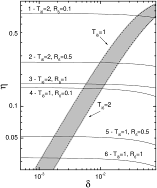
Figure 1: Potential shielding factor $\eta$ calculated from Eq. (5) - two dashed lines, and from Eq. (11) - six solid lines numbered from 1 to 6, versus the temperature difference $\delta=(T_{i}-T_{s})/10^{6}$ K, where $T_{i}$ is the ion critical temperature (Eq. (2)) and $T_{s}<T_{i}$ is the actual surface temperature.

Figure 1 shows values of the shielding factor $\eta$ calculated from Eqs. (5) represented by two dashed lines, and (11), represented by six numbered solid lines. We introduced a parameter $\delta=T_{i6}-T_{6}$ shown on the horizontal axis, which describes a difference between the iron critical temperature $T_{i}=T_{i6}\times 10^{6}$ K and the actual surface temperature $T_{s}=T_{6}\times 10^{6}$ K. Using this parameter we can rewrite Eq. (5) in the form $\eta=1-exp\left[-30\delta/(T_{i6}-\delta)\right]$, and two dashed lines presented in Fig. 1 correspond to limiting values $T_{i6}=$1 and 2, respectively. Similarly, Eq. (11) can be rewritten in the form $\eta=3.25\times 10^{-2}(T_{i6}-\delta)^{7/3}{\cal R}_{6}^{-2/3}P_{1}^{-1/3}$, and six numbered lines presented in Fig. 1 correspond to different (indicated) combinations of $T_{i6}$ and ${\cal R}_{6}$ values ($P_{1}=1$ was used in all cases). The actual values of $\eta$ correspond to the shadowed region limited by the two dashed lines and the two numbered lines 1 and 6 from the top and the bottom, respectively. If the iron critical temperature $T_{i}$ is not much lower than $10^{6}$ K and (3)) and ${\cal R}_{6}$ is not much smaller than 0.1, then the value of $\eta$ should lie in the range 0.03-0.8. This suggests that the actual value of the parameter $\delta$ should range between a fraction of a percent to several percent at most. We therefore conclude that a difference between $T_{i}$ and $T_{s}$ (or $T_{e}$ and $T_{s}$) should be of the order of $10^{4}$ K. In the next section we constrain both $T_{i}$ (or $T_{e}$) and $T_{s}$ from the observationally deduced drift-rates for a number of pulsars. The inferred surface temperature $T_{s}$ and the difference between $T_{i}$ (or $T_{e}$) and $T_{s}$ agree very well with a general estimate obtained here.

The model of a charge-depleted acceleration region described by Eqs. (1) and Eq. (5) for ions and Eq. (7) for electrons is highly sensitive to both $T_{i,e}$ and $T_{s}$ temperatures, where $T_{i,e}$ means either $T_{i}$ (Eqs. (3), (4)) or $T_{e}$ (Eq. (8)). The inequality $T_{s}<T_{i,e}$ is often used as a thermal condition for the “vacuum gap formation” (GM00; GM02; Abrahams & Shapiro as91 (1991); Usov & Melrose um95 (1995), um96 (1996)) and its exact meaning is worth understanding. When the surface temperature $T_{s}$ is only 10% below $T_{i,e}$, then $\eta\approx 0.95$, that is $\rho_{i,e}$ is only a few percent of the corotational GJ charge density and the situation is close to the pure vacuum case of RS (see discussion below Eq. (8) in CR80 for details). If this is the case, then the potential drop $\Delta V\approx\Delta V_{max}$ is being screened mostly due to the intense production of $e^{-}e^{+}$ pairs, that is, the total charge density $\rho_{t}\leq\rho_{GJ}$ (equality holds when a spark plasma filament is fully developed), where $\rho_{t}=\rho_{i}+\rho_{+}$ or $\rho_{t}=\rho_{e}+\rho_{-}$, and $\rho_{+}$ and $\rho_{-}$ are charge densities of positrons and electrons produced in $e^{-}e^{+}$ pairs in spark discharges, respectively. The back flow of high density electrons or positrons accelerated to relativistic energies by the vacuum potential drop, heats strongly the surface beneath the sparks. As a result, the surface temperature $T_{s}$ increases, which may intensify the thermionic ion/electron outflow, additionally screening the potential drop to the level $\Delta V=\eta\Delta V_{max}$. At this stage, the cooling process should slightly dominate, because of weaker heating due to the back flow of lower density $\rho_{\pm}=\eta\rho_{GJ}$ and lower energy $\gamma=\eta\Delta V_{max}/m_{e}c^{2}$ electrons/positrons. Thus, the actual surface temperature should be thermostatically self-regulated. If heating and cooling are nearly in balance, then the quasi-equilibrium surface temperature $T_{s}$ is very close to $T_{i}$ (Fig. 1), with the difference being less than about 1%. Thus, contrary to the suggestion of CR80 (see discussion below their Eq. (8)), the conditions close to a pure vacuum gap will never be established in the quasi-equilibrium stage. Nevertheless, the potential drop arising due to a small charge depletion above the polar cap is high enough for the non-stationary sparking scenario to be realized in the way similar to that envisioned by RS.

The sparking discharge terminates if the total charge density $\rho_{t}=\rho_{i,e}+\rho_{\pm}$ reaches the GJ value (Eq. (1)), where $\rho_{i,e}$ is described by Eqs. (5) and (7), respectively, and time dependent $\rho_{\pm}(t)$ is the charge density of produced electrons/positrons. A slight adjustment to $\rho_{i,e}$ is also expected in the final stage of a spark development due to the surface temperature variations. More exactly, the discharge terminates when the screened potential drop $\Delta V=(1-\rho_{t}/\rho_{GJ})\Delta V_{max}=(\eta-\rho_{\pm}/\rho_{GJ})\Delta V_{max}$ falls below the threshold value $\Delta V_{min}=\gamma_{min}(mc^{2}/e)\approx 2.5\times 10^{3}T_{6}^{1/3}{\cal R}^{1/3}(mc^{2}/e)\approx 5\times 10^{8}$ V, inhibiting further $e^{-}e^{+}$ pair production (see Appendix A.1. for determination of $\Delta V_{max}$ and $\gamma_{min}$). Since $\Delta V_{max}=\Delta V_{ICS}\sim(10^{11}-10^{12})$ V (see Eq. (11) in GM02 or Eq. (A.6) in this paper), then $\Delta V_{min}/\Delta V_{max}\sim 10^{-3}\approx(\eta-\rho_{\pm}/\rho_{GJ})$. Therefore, the discharge terminates if $\rho_{\pm}=\eta\rho_{GJ}$, which can be a small fraction of GJ density. In fact, the condition $\gamma_{acc}>\gamma_{min}$ leads to a lower limit $\eta>10^{-4}b{\cal R}_{6}^{-1}T_{6}$, where $\gamma_{acc}$ is determined in Eq. (A.15). Since the product $b{\cal R}_{6}^{-1}$, describing small scale anomalies of the surface magnetic field should be about 10, the absolute lower limit for $\eta$ is about 0.001. It should be obvious from the above considerations that the sparking discharge can proceed in a similar way to that envisioned by RS, even if the parameter $\eta$ is very low, say below 0.01. In reality, however, one should expect that typically $\eta$ is of the order of 0.1 (Fig. 1) and thus $\rho_{i,e}\sim 0.9\rho_{GJ}$. Thus, one can say that the sparking discharge begins at the partially shielded potential drop $\Delta V\sim 0.1\ \Delta V_{max}\sim 10^{10}-10^{11}$ V and terminates when this potential drop is largely reduced by about two orders of magnitude (due to the screening by cascading production of $e^{-}e^{+}$ pairs).

At the final stage of a spark development, when heating is most intense, the maximum polar cap temperature that can be achieved is $T_{s}=T_{i,e}$ and the spark discharge is terminated. Then, in the absence of heating from a pair production mechanism, the surface temperature should drop fast enough to enable the next discharge to recur within a sufficiently short amount of time. The e-folding cooling time $\tau_{cool}$ is estimated in Appendix B.2. as being of the order of 1 $\mu$s (Eq. B.14). Thus, the surface temperature can drop by a factor of $e$ in a time interval of the order of $\sim\mu$s. However, in our scenario it is only required that the temperature drops by a few to several percent, and thus a corresponding cooling time is at least 10 times shorter. This is comparable with a gap emptying time (or transit time) $t\sim h/c$, which is of the order of 100 ns or less (e.g. Asseo & Melikidze am98 (1998), GS00). On the other hand, the heating time scale due to electron/positron bombardment is about $(10-40)h/c$ (RS, see also Appendix B.3.). Therefore, sparking discharges should be easily able to cycle on and off on a natural thermal timescales, comparable to those described by RS model of a spark development (exponentiation of charge density from $\rho\approx 0$ to $\rho=\rho_{GJ}$).

4 Subpulse drift in pulsars

We now compare the observationally deduced drift-rates with theoretical predictions of the ${\bf E}\times{\bf B}$ drift model determined by Eqs. (A.13–A.15). The input parameters and the observationally deduced parameters are summarized in Table 1. The most important are: the drift periodicity $P_{3}$ and the circulational (tertiary) periodicity $\hat{P}_{3}$, which are related to each other by the number of circulating sparks $N=\hat{P}_{3}/P_{3}$. If necessary/possible these values are corrected for aliasing effects. In the first three cases listed in Table 1 we rely on a robust analysis of real observational data, while in the next three cases (PSRs 2303+30, 2319+60 and 0031-07) we deduce drift parameters by reproducing the actual pulse sequences using the simulation model and fitting the free model parameters to the observed values (see GS00 for details).

4.1 PSR 0943+10

This pulsar was extensively analyzed and interpreted recently by DR99, DR01, Asgekar & Deshpande (2001) and Gil & Sendyk (2003). These authors revealed clearly that drifting subpulses in this pulsar result from a system of $N=20$ subbeams (sparks) circulating around the magnetic axis at the periphery of the pulsar beam (polar cap). Each subbeam (spark) completes one full circulation in $\hat{P}_{3}=37.35P_{1}$, therefore $P_{3}=\hat{P}_{3}/N=1.87P_{1}$, where $P_{1}$ is the pulsar period. These precise estimates were possible due to the successful resolving of aliasing near the Nyquist frequency $f_{3}\sim 0.5/P_{1}$ (or $P_{3}\sim 2P_{1}$).

At the periphery of the polar cap the circulation distance $d\approx r_{p}-h$, where $r_{p}$ is the polar cap radius (Eq. (15)) and $h$ is the height of the acceleration region (e.g. Eqs. (19) and (20)). Thus equation (23) gives in this case $\hat{P}_{3}=\eta^{-1}P_{1}[(r_{p}/h)-1]$. In order to compare this equation with the observed value $\hat{P}_{3}=37.35P_{1}$, we have to estimate the complexity parameter $r_{p}/h$, representing the ratio of the polar cap radius to the characteristic spark dimension ${\cal D}\sim h$ at the polar cap periphery (GS00). First, let as assume after RS that the typical distance between adjacent sparks at the periphery of the polar cap is also about $h$. If this is the case, then $2\pi d=2\pi(r_{p}-h)=2Nh$, which leads to $r_{p}/h-1=N/\pi=20/\pi$ or $r_{p}/h\approx 7.4$ (see also GMM02b who obtained $r_{p}/h=7.34\pm 0.8$ for this pulsar; in consistence with approximate Eq. (11) in GS00, which gives $r_{p}/h=6.8$). Therefore, with $r_{p}/h=7.4$ we obtain $\hat{P}_{3}=6.4P_{1}/\eta=37.35P_{1}$, which gives the value of the shielding parameter $\eta=0.17$, that can be compared with theoretical predictions using Eq. (5) or (7) for partial electron flow of ions or electrons, respectively.

The actual quasi-equilibrium surface temperature is described by Eq. (11), which for $\eta=0.17$ and ${\cal R}_{6}=1$ gives $T_{s}=1.646\times 10^{6}$ K. On the other hand, from Eqs. (5) and (7) we obtain $T_{i}/T_{s}=1.00625$ and $T_{e}/T_{s}=1.0075$, which gives critical iron $T_{i}=1.656\times 10^{6}$ K and electron $T_{e}=1.658$ K temperatures, respectively. Note that $\Delta T=T_{i}-T_{s}\sim T_{e}-T_{s}\sim 10^{4}$ K, in agreement with the general prediction made in Sect. 3. The comparison of $T_{i}$ with Eq. (3) and (4) for iron critical temperatures and $T_{e}$ with Eq. (8) for electron critical temperature implies that $b=2.8$, 29.7 and 18 or $B_{s}\simeq 10^{13}$ G, $B_{s}=11.2\times 10^{13}$ G and $B_{s}=7\times 10^{13}$ G, respectively. As one can see, the calculations of the cohesive energy by Jones (j86 (1986)) represented by Eq. (4) lead to values of $B_{s}$ largely exceeding the critical quantum field $B_{q}=4.4\times 10^{13}$ G, which is believed to represent the photon splitting limit above which the plasma necessary for generation of pulsar radio emission can not be produced (e.g. Zhang & Harding 2002 and references therein). On the other hand, calculations of Abrahams & Shapiro (as91 (1991)) for the iron critical temperature represented by Eq. (3) give a quite suitable value of the surface magnetic field $B_{s}\sim 10^{13}$ G (Table 1). The electron case represented by Eq. (8) can be ruled out, since the corresponding $B_{s}=7\times 10^{13}$ G exceeds largely the photon splitting limit.

4.2 PSR B0809+74

This pulsar was recently analyzed by van Leeuwen et al. (vl03 (2003)), who argued that the number of circulating beams $N\geq 15$ and the circulation period $\hat{P}_{3}>150P_{1}$. Assuming again that the observed drifting subpulses in this pulsar correspond to the periphery of pulsar beam (polar cap) we have $\hat{P}_{3}=\eta^{-1}P_{1}[(r/h)-1]$ and $r_{p}/h=(N/\pi)+1\raisebox{-1.29167pt}{\mbox{$\stackrel{{\scriptstyle>}}{{{}_{\sim}}}\,$}}5.8$ (see Sect. 4.1). Thus, the shielding factor $\eta>0.032$ and using Eq. (5) we obtain $T_{i}/T_{s}=1.001$, while Eq. (7) gives $T_{e}/T_{s}=1.0013$. The actual surface temperature can be estimated from Eq. (11), which for $\eta=0.032$ and ${\cal R}_{6}=1$ gives $T_{s}=0.955\times 10^{6}$ K. Therefore we have $T_{i}=0.956\times 10^{6}$ K and $T_{e}=0.957\times 10^{6}$ K, respectively (notice that in this case $\Delta T=T_{i}-T_{s}=T_{e}-T_{s}\sim 2\times 10^{3}$ K). These values can now be compared with Eqs. (3), (4) and (8), which give $B_{s}=4\times 10^{12}$ G (less than the minimum value $0.1B_{q}$ required by near-threshold conditions described in Appendix A.1.), $B_{s}=3\times 10^{13}$ G (too close to $B_{q}$) and $B_{s}=7\times 10^{12}$ G, respectively (OK). The latter value of the surface magnetic field is very suitable, suggesting that PSR 0809+74 is a good candidate for a drifting subpulse pulsar with a positively charged polar cap (antipulsar in the terminology of RS).

4.3 PSR B0826-34

The drifting subpulses in this remarkable pulsar were first observed by Biggs et al. (betal85 (1985)). The average profile is very broad and consist of the main-pulse (MP) and the interpulse (IP). The single pulse emission occurs practically at every longitude of the 360 degrees pulse window, implying that this pulsar is an almost aligned rotator (i.e. the inclination angle $\alpha$ between the rotation and magnetic axes is very small). At 645 MHz Biggs et al. (betal85 (1985)) revealed 5 to 6 bands of drifting subpulses, swinging across the MP window. Individual subpulses show a variable drift rate, including changes of the apparent drift direction approximately every 100 pulses (see Fig. 2 in Biggs et al. 1985). Such patterns of drifting subpulses are inconsistent with the ${\bf E}\times{\bf B}$ drift model, unless the observed effects result from aliasing and small changes in the drift-rate causing $P_{3}$ to fluctuate around the relevant Nyquist boundary (as in the case of PSR 2303+30; see Fig. 3 in GS00). Recently Gupta et al. (getal03 (2003)) attempted to resolve the possible aliasing in PSR 0826-34. They reobserved this pulsar at 318 MHz using the GMRT and obtained a sequence of 500 good quality single pulses. At this frequency 6 to 7 bands of drifting subpulses appeared, behaving similarly to those 5-6 bands observed by Biggs et al. (betal85 (1985)) at a higher frequency. The careful analysis revealed that subpulse-associated sparks circulate always in one direction consistent with the ${\bf E}\times{\bf B}$ drift model, but the observed patterns are determined by the aliasing corresponding to $P_{3}\sim P_{1}$ (thus around the fluctuation frequency $f_{3}\sim 1/P_{1}$).

The observed longitudinal drift rate $D_{0}=d\varphi/dt=P_{2}/P_{3}$ corrected for aliasing $(P_{3}\sim P_{1})$ is $D_{0}\approx P_{2}/P_{1}$, where $P_{2}\approx 26^{\circ}$ is the typical distance between adjacent subpulses, where $\varphi$ is the observed subpulse longitude. The circulational periodicity $\hat{P}_{3}=360^{\circ}/D_{r}$, where $D_{r}=d\chi/dt$ is the intrinsic azimuthal drift rate (see Appendix A.2.). In the case of an almost aligned rotator $(\alpha\sim 0^{\circ})$ one can write $D_{r}\sim D_{0}=26^{\circ}/P_{1}$ and thus $\hat{P}_{3}\approx(360^{\circ}/26^{\circ})P_{1}=13.85P_{1}$. Therefore, in PSR 0826-34 there are $N=\hat{P}_{3}/P_{3}\approx\hat{P}_{3}/P_{1}=14$ sparks circulating around the pole at the rate $D_{r}\approx 26^{\circ}/P_{1}$.

The detailed analysis of single pulses performed by Gupta et al. (getal03 (2003)) revealed also that sparks contributing to the MP emission of B0826-34 circulate at $d\sim 0.5r_{p}$ (the middle of the polar cap), while the IP emission occupies the periphery of the polar cap. Thus, according to Eq. (23) with $s=0.5$, the circulation period $\hat{P}_{3}=\eta^{-1}P_{1}(0.5r_{p}/h)^{2}$, which can be compared with the observationally deduced value $\hat{P}_{3}\sim 14P_{1}$. To estimate the value of $(r_{p}/h)$ let us notice that in this case $2\pi d=2N{\cal D}$, where $d\sim 0.5r_{p}$ and ${\cal D}\sim 0.5h$ is the characteristic spark dimension in this region of the polar cap. Therefore $r_{p}/h=N/\pi=14/\pi\sim 4.5$, thus $\hat{P}_{3}=5\eta^{-1}P_{1}\approx 14P_{1}$ and, in consequence, the shielding factor $\eta=0.357$. Now using Eqs. (5) and (7) we obtain $T_{i}/T_{s}=1.0147$ and $T_{e}/T_{s}=1.0188$, respectively. The actual surface temperature can be estimated from Eq. (10), which for ${\cal R}_{6}=1$ and $\eta=0.36$ gives $T_{s}=2.565\times 10^{6}$ K. Consequently, we get $T_{i}=2.469\times 10^{6}$ K and $T_{e}=2.475\times 10^{6}$ K, respectively (note that $\Delta T=T_{i}-T_{s}\approx T_{e}-T_{s}\sim 3\times 10^{4}$  K). Comparing these critical temperatures with Eqs. (3), (4) and (9) we obtain $B_{s}=1.4\times 10^{13}$ G, $1.5\times 10^{15}$ G and $5\times 10^{13}$ G, respectively. Thus, again the calculations of the cohesive energy by Abrahams & Shapiro (as91 (1991)) represented by Eq. (3) seem to be the most adequate, while the calculations of Jones (j86 (1986)) lead to $B_{s}>10^{15}$ G. Also the electron case with $B_{s}=5\times 10^{13}\leavevmode\nobreak\ {\rm G}>B_{q}$ can be excluded in this case.

The observed time variability of the apparent drift rate, including the change of the apparent drift direction in PSR B0826-34 can be explained by time variations of the shielding factor $\eta$ (Eqs. (5), (7), (A.7) and (A.8)), which, according to Eq. (11), implies a time variability of the surface temperature $T_{s}$. The detailed analysis of sequences of drifting subpulses in PSR 0826-34 performed by Gupta et al. (getal03 (2003)) indicates the following variations over about 100 pulse sequences: the azimuth drift rate $D_{r}$ varies from $25^{\circ}/P_{1}$ to $27^{\circ}/P_{1}$, drift velocity $v_{d}$ from 7.5 m/s to 9 m/s, $P_{3}$ from 1.03$P_{1}$ to 0.95$P_{1}$ and $\hat{P}_{3}$ from 14.4$P_{1}$ to 13.3$P_{1}$. The change of the apparent drift direction due to aliasing occurs when $P_{3}=1.0P_{1}$ and thus $\hat{P}_{3}=14P_{1}$. These approximately 100 pulse cycles repeat in a quasi-periodic manner. During each cycle the shielding factor increases by a few percent (around $\eta=0.36$) and the surface temperature drops by about 2000 K (around $T_{s}=2.47\times 10^{6}$ K). Notice that similar (though erratic) variations of these parameters, with an amplitude of about a few percent, were observed in PSR 0943+10 (see footnote 3).

4.4 PSR 2303+30

GS00 reproduced the drifting subpulses in this pulsar (see their Fig. 3) and argued that in this case $r_{p}/h\sim 5$, $N=12$ and $\hat{P}_{3}\approx 23P_{1}$, which is consistent with $P_{3}\sim 1.9P_{1}$ obtained by Sieber & Oster (so75 (1975)). For the periphery of the polar cap we get $\eta=0.16$, $T_{s}=1.854\times 10^{6}$ K, $T_{i}=1.864\times 10^{6}$ K and $T_{e}=1.865\times 10^{6}$ K. Comparison with Eqs. (3), (4) and (8) gives $B_{s}=9.6\times 10^{12}$ G (OK), $B_{s}=8.7\times 10^{13}$ G (too high) and $B_{s}=3.7\times 10^{13}$ G (probably too high), respectively. Thus again, the calculations of the cohesive energy by Abrahams & Shapiro (1991) seem to be most adequate.

This pulsar also shows an apparent change of the subpulse drift direction (see Fig.  3 in GS00), which can be explained by small changes of: the azimuth drift-rate from $14.^{\circ}4/P_{1}$ to $15.^{\circ}5/P_{1}$, the drift velocity $v_{d}$ from $\sim 10$ m/s to $\sim 11$ m/s, $P_{3}$ from 2.1$P_{1}$ to $1.9P_{1}$ and $\hat{P}_{3}$ from $25P_{1}$ to $23P_{1}$ (notice, that similar variations of these parameters were observed in PSRs 0826-34 and 0943+10). The corresponding change of the shielding factor $\eta$ is about one percent, which implies the change of the surface temperature $T_{s}$ of about 1000K (around $T_{s}=1.85\times 10^{6}$ K).

4.5 PSR 2319+60

GS00 reproduced the drifting subpulses in this pulsar (see their Fig. 4) and argued that in this case $N=9$, $\hat{P}_{3}\sim 70P_{1}$, $P_{3}\sim 7.8P_{1}$ and $r_{p}/h\sim 5$. For sparks drifting at the periphery of the polar cap we get $\eta\sim 0.071$, $T_{s}=1.236\times 10^{6}$ K, $T_{i}=1.239\times 10^{6}$ K and $T_{e}=1.239\times 10^{6}$. Comparison with Eqs. (3), (4) and (8) gives $B_{s}\sim 5\times 10^{12}$ G (this value is lower than $B_{d}=8\times 10^{12}$ G and should be rejected), $B_{s}=5\times 10^{13}$ G (this value is higher than the photon splitting limit $B_{q}$ and should also be rejected) and $B_{s}=1.36\times 10^{13}$ G. Thus, only the latter case seams acceptable and therefore PSR 2319+60 should be considered as the pulsar with a negatively charged polar cap (antipulsar in RS terminology).

4.6 PSR 0031-07

GS00 reproduced drifting subpulses in this pulsar (see their Fig. 5) and argued that in this case $N\geq 5$, $\hat{P}_{3}>34P_{1}$, $P_{3}\sim 6.8P_{1}$ and $r_{p}/h\sim 4$. For the peripheral sparks we get $\eta>0.089$, $T_{s}=1.551\times 10^{6}$ K, $T_{i}=1.556\times 10^{6}$ K and $T_{e}=1.557\times 10^{6}$ K. Comparison with Eqs. (3), (4) and (8) gives $B_{s}=7.2\times 10^{12}$ G (OK), $B_{s}=7.9\times 10^{13}$ G (too high) and $B_{s}=2.2\times 10^{13}$ G (probably too high). Thus again, the calculations of cohesive energy of Abrahams & Shapiro (1991) seem to be most adequate and calculations by Jones (1986) are not suitable within our model.

5 Discussion and conclusions

Recent progress in the analysis of drifting subpulses in a number of pulsars (DR99, DR01, Asgekar & Deshpande 2001, van Leeuwen et al. 2002, GMM01b, Gil & Melikidze 2002 and Gil & Sendyk 2003) provided a strong support to the canonical RS pulsar model, which relates the spark plasma filaments with subpulse-associated subbeams of radio emission. The observed subpulse drift is naturally explained by the inevitable ${\bf E}\times{\bf B}$ drift of these plasma filaments, at least qualitatively. However, on the quantitative level, the ${\bf E}\times{\bf B}$ drift in a pure vacuum gap is too fast as compared with observations. In this paper, we consider a general concept of the charge depletion region (rather than a pure vacuum gap), with a thermal outflow of ${}^{56}_{26}$Fe ions, coexisting with the generation of $e^{-}e^{+}$ plasmas (CR80). The presence of an ion flow decreases the accelerating gap potential drop and, in consequence, the ${\bf E}\times{\bf B}$ drift-rate, as well as the amount of surface heating due to back-flowing relativistic electrons (positrons). As originally demonstrated by CR80, the extreme sensitivity of the potential drop to the surface temperature makes the gap thermostatically self-regulating, whenever there is both an ion outflow and $e^{-}e^{+}$ discharge plasma. We argued that when heating and cooling are nearly in balance, the surface temperature $T_{s}$ oscillates within a very narrow range around its quasi-equilibrium value, slightly below the critical temperature $T_{i}$ ($T_{e}$) above which the ion outflow reaches the co-rotational GJ density.

Our general model of the charge depleted acceleration region can be applied not only to pulsars with positively charged polar caps $({\bf\Omega}\cdot{\bf B}<0)$, but also to pulsars with negatively charged polar caps $({\bf\Omega}\cdot{\bf B}>0)$, which are usually interpreted within the so-called stationary flow models (e.g. Arons 1981 and references therein) in which electrons flow freely from the polar cap surface at the GJ charge density. Within the model of a partially shielded acceleration region the ${}^{56}_{26}$Fe ions are only marginally bound at a temperature $T_{s}\raisebox{-1.29167pt}{\mbox{$\stackrel{{\scriptstyle<}}{{{}_{\sim}}}\,$}}T_{i}$, but, nevertheless, the non-stationary sparking scenario can be realized in a way similar to that envisioned by RS in their pure vacuum gap model (with strong binding assumed). We suggest that such marginally bound ions are not much different from marginally bound electrons (at $T_{s}\sim T_{e}$). In fact, RS-type non-stationarity (sparks) can also arise if the thermionic electron flow from the surface is not exactly at the GJ corotational charge density. As we demonstrated, even small departures from GJ charge density at the surface temperature $T_{s}\approx T_{e}$ can result in the sparking discharge of the shielded accelerating potential drop above the polar cap. Thus we suggest that both pulsars with positively and negatively charged polar caps can develop non-stationary inner acceleration regions, similar to those invoked by RS. In consequence, the spark-associated coherent radio emission due to instabilities in the non-stationary $e^{-}e^{+}$ secondary plasma (e.g. Usov 1987, Asseo & Melikidze 1991, Melikidze et al. 2000) may originate similarly in both pulsars $({\bf\Omega}\cdot{\bf B}<0)$ and “antipulsars” $({\bf\Omega}\cdot{\bf B}>0)$.

We estimated values of the polar cap surface temperature for six pulsars (Table 1). The estimated values of $T_{s}$ lie in the range between $\sim 1.0$ to $\sim 2.5$ million K. It is worth noting that in a pure vacuum gap (in RS with $\eta=1$), the values of $T_{s}$ would be higher by a factor of about 2, thus in some pulsars from our list exceeding $4\times 10^{6}$ K at the polar cap. Present and future x-ray satellite spectral measurements should be able to constrain maximum surface temperatures of the polar cap heated by intense spark discharges. One should also mention that our estimates of $T_{s}$ were obtained under canonical assumptions that ${\cal R}_{6}=1$ (e.g. RS). However, if the radius of curvature of surface magnetic field lines is much smaller than $10^{6}$ cm, then the values of $T_{s}$ can be lowe even by a factor $2-3$. Thus, our estimates of $T_{s}$ presented in Table 1 represent the upper limits.

Our method is capable of determing both the actual surface temperature $T_{s}$ and critical temperature $T_{i}$ or $T_{e}$, above which the thermionic emission of iron ions or electrons reaches the corotational GJ value. We found that radio pulsars operate at $T_{s}$ approximately $10^{4}$ K lower than $T_{i}$ or $T_{e}$. Comparing our observationally deduced values of critical temperatures with estimates based on the calculations of the cohesive energy and/or work function, we found the required values of the surface magnetic field $B_{s}=bB_{d}$ (Table 1). Within our model we can exclude the calculations of the cohesive energy by Jones (j86 (1986)), represented in our paper by Eq. (4). In most cases calculations of Abrahams & Shapiro (as91 (1991)) represented by Eq. (3) give suitable results, except PSR 0031-07 which is the best candidate for drifting subpulse pulsars with a negatively charged polar cap. Also PSR 0869+74 seems to belong to this category. Interestingly, these two pulsars require the lowest shielding factors $\eta$ (Table 1) to fit the observed and the theoretical drift-rates.

The sparks rotate due to the ${\bf E}\times{\bf B}$ drift in the same direction as the neutron star rotates (lagging behind the polar cap surface). As a matter of fact, the particle drift in the inertial frame cannot exceed the stellar rotation speed within any reasonable model. Thus, the observed direction of the subpulse drift is fixed for a given pulsar and depends only on whether the line-of-sight trajectory passes poleward or equatorward of the magnetic axis. However, two pulsars from our sample demonstrate an apparent change of the drift direction. We argued that sense-reversals can be explained by small changes of the drift-rate causing the $P_{3}$ value to fluctuate around the relevant Nyquist boundary: $P_{3}\approx 1P_{1}$ in the case of PSR 0826-34 and $P_{3}\sim 2P_{1}$ in case of PSR 2303+30, corresponding to fluctuation frequencies $f_{3}$ equal to 1 cycle/$P_{1}$ and 0.5 cycle$/P_{1}$, respectively. We believe that these changes are due to small variations of the polar cap surface temperature. PSR 0540+23 probably also belongs to the category of pulsars with $P_{3}\approx 1P_{1}$, showing apparent reversals of the sense of subpulse drift (Nowakowski 1991), although its drifting patterns are much more chaotic than in PSR 0826-34.

Up to now, it was believed that in conal profiles (Rankin 1983) the values of $P_{3}$ periods covered the range from about 2 to about 15 pulsar periods $P_{1}$ (corresponding to fluctuation frequencies between about $0.5/P_{1}$ (Nyquist frequency) to about $0.07/P_{1}$). It is well illustrated in Fig. 4 and Table 2 in Rankin (1986). In this paper we broadened this range by adding at least one pulsar PSR 0826+23 with $P_{3}\sim P_{1}$ (Table 1), and probably PSR 0540+23 (Nowakowski 1991) also belongs to this category. Perhaps there are many more pulsars with a fast drift corresponding to $P_{3}$ values well below “Nyquist limit”.

It is worth emphasizing again that the subpulse drift is widely considered as a crucial clue towards solving the long standing mystery of pulsar radio emission. Despite its potential importance, this phenomenon has not attracted much theoretical attention beyond that of RS model. A simple explanation of this fact is that probably it is very difficult to propose a theory that would be as natural as the RS model, at least qualitatively. Moreover, this is the only model offering quantitative predictions that can be compared with observations. We review in this paper a number of problems appearing when the existing theory is confronted with the current pulsar data and argue that all of them disappear when the original RS model is modified to include a thermionic outflow of ions or electrons, coexisting with the electron-positron plasma produced in spark discharges. We also emphasize the importance of the strong non-dipolar surface magnetic field driving the spark avalanches, as well as resonant inverse Compton scattering as the mechanism providing seed photons for these avalanches.

Finally, we believe that the phenomenon of drifting subpulses is a manifestation of a more general phenomena related to sparking discharges of the ultra-high potential drop above the polar cap of radio pulsars. Therefore, the result of this paper strongly suggest that spark-associated plasma instabilities (Usov 1987, Asseo & Melikidze 1998) play an important role in generation of the observed coherent pulsar radio emission (e.g. Melikidze et al. 2000).

Appendix A Inner acceleration region

A.1 Charge depleted acceleration region above the polar cap

The acceleration potential drop above the polar cap results from the deviation of a local charge density $\rho$ from the corotational GJ density

$$\rho_{GJ}=-\frac{{\bf\Omega}\cdot{\bf B_{s}}}{2\pi c},$$ (12)

where ${\bf\Omega}$ is the pulsar spin vector and ${\bf B}(r)$ is the pulsar magnetic field, which should be purely dipolar at altitudes of a few stellar radii $R_{*}=10^{6}$ cm, where the pulsar radio emission is expected to originate (e.g. Kijak & Gil 1998 and references therein), but could be highly nondipolar (i.e. having a pronounced small-scale spatial structure) at the polar cap surface. For reasons of generality we describe the surface magnetic field by

$$B_{s}=bB_{d},$$ (13)

where

$$B_{d}=2\times 10^{12}(P_{1}\dot{P}_{-15})^{0.5}\leavevmode\nobreak\ {\rm G}$$ (14)

is the dipolar component of the pulsar magnetic field at the pole, $P$ is the pulsar period in seconds and $\dot{P}_{-15}=\dot{P}/10^{-15}$ and $b>1$. This defines the actual radius of the polar cap

$$r_{p}=b^{-0.5}10^{4}P_{1}^{-0.5}\leavevmode\nobreak\ {\rm cm},$$ (15)

(e.g. GS00). We also introduce the curvature radius of nondipolar surface magnetic field lines ${\cal R}_{6}={\cal R}/R_{*}\raisebox{-1.29167pt}{\mbox{$\stackrel{{\scriptstyle<}}{{{}_{\sim}}}\,$}}1$, where $R_{*}=10^{6}$ cm is the neutron star radius (note that for a purely dipolar field $R_{6}\sim 300$ near the polar cap). Within our model of the charge depleted region the local charge density $\rho=(1-\eta)\rho_{GJ}$, where $\eta=1-\rho_{i}/\rho_{GJ}$ (or $\eta=1-\rho_{e}/\rho_{GJ}$) and $\rho_{i}$ (or $\rho_{e}$) is the charge density of outflowing thermionic ions (or electrons). Within the acceleration region the potential $V$ and the electric field $E$ (parallel to the magnetic field ${\bf B_{s}}$) are determined by one-dimensional Poisson equation $d^{2}V/dz^{2}=-4\pi(\rho-\rho_{GJ})=4\pi\eta\rho_{GJ}$, with the boundary condition $dV/dz=0$ at $z=h=h_{max}$ and $dV/dz=E_{max}$ at $z=0$ (see below for determination of $h$). Since $\rho_{GJ}\approx\pm B_{s}/cP$, where the sign $+(-)$ corresponds to the ion (electron) flow, the solution of Poisson equation gives $E(z)=\pm\eta(4\pi/cP_{1})B_{s}(h-z)$ and $\Delta V=\int_{0}^{h}E(z)dz=\pm\eta(2\pi/cP_{1})B_{s}h^{2}$ or

$$\Delta V=\pm\eta\Delta V_{max},$$ (16)

where

$$\Delta V_{max}=\frac{2\pi}{cP_{1}}B_{s}h^{2}$$ (17)

is the acceleration potential drop within a pure vacuum gap (RS) corresponding to $\eta=1$ ($\rho_{i}=0$ or $\rho_{e}=0$).

The height $h$ of the acceleration region with ultra-high potential drop $\Delta V$ described by Eqs. (A.1) and (A.2) is determined by a quasi-steady discharge via magnetic conversion of high energy $\hbar\omega>2mc^{2}$ photons into $e^{-}e^{+}$ pairs that develop cascading sparks. Thus $h=l_{ph}$, where $l_{ph}$ is the mean free path of an energetic photon to produce a pair. At least several possible models of the inner acceleration region were considered by different authors (see Zhang et al. 2000; ZHM00 hereafter and GM02 for review). Among them, the most promising one with respect to the possibility of creating an effective acceleration region (“vacuum gap”) seems to be the Near-Threshold $(\hbar\omega=2mc^{2}{\cal R}/l_{ph})$ model, involving the resonant ICS seed photons $(\hbar\omega=2\gamma\hbar eB_{s}/mc)$ in the strong magnetic field $B_{s}>0.1B_{q}\sim 5\times 10^{12}$ G (see GM01 and GM02 for details of the so-called ICS-NTVG model). Unlike in the RS case with curvature seed photons, the mean free path of ICS seed photons in ICS-NTVG model is approximately equal to the mean electron path $l_{e}=0.0027\gamma^{2}B_{12}^{-1}T_{6}^{-1}$ to emit an energetic photon with energy $\hbar\omega=2\gamma\hbar eB/mc$ exceeding a pair formation threshold (ZHM00, GM01, GM02), where $B_{12}=B_{s}/10^{12}$ G. Since $2mc^{2}{\cal R}/h=2\gamma\hbar eB_{s}/mc$, then the minimum Lorentz factors $\gamma$ required for the ICS dominated pair production under the Near Threshold conditions is

$$\gamma_{min}=(2.18\times 10^{7})b^{-1}{\cal R}_{6}h^{-1}(P\dot{P}_{-15})^{-0.5},$$ (18)

(see Eq. (2) and GM01 and references therein for details). Now using $h_{ICS}=h=l_{e}$ with $\gamma=\gamma_{min}$ we can obtain the expression for the height of the ICS dominated acceleration region with a strong magnetic field

$$h_{ICS}=(8.6\times 10^{3}){\cal R}_{6}^{2/3}b^{-1}(P\cdot\dot{P}_{-15})^{-1/2}T_{6}^{-1/3}\leavevmode\nobreak\ {\rm cm}$$ (19)

and thus $\gamma_{min}\approx 2.5\times 10^{3}T_{6}^{1/3}{\cal R}_{6}^{1/3}$, which reproduces Eq. (10) in GM02

$$h_{ICS}=(5\times 10^{3}){\cal R}_{6}^{0.57}b^{-1}P^{-0.36}\dot{P}_{-15}^{0.5}\leavevmode\nobreak\ {\rm cm},$$ (20)

if $T_{6}=T_{s}/10^{6}$ K is expressed by their Eq. (12) and $\eta=\xi=k=1$. According to Eqs. (2), (A.1) and (A.2), the acceleration potential drop is

$$\Delta V=(8\times 10^{12})\eta b^{-1}{\cal R}_{6}^{4/3}T_{6}^{-2/3}P^{-3/2}\dot{P}_{-15}^{-1/2}\leavevmode\nobreak\ V,$$ (21)

which reproduces Eq. (11) in GM02

$$\Delta V_{ICS}=(5.2\times 10^{12}){\cal R}_{6}^{1.14}b^{-1}P^{-1.22}\dot{P}_{-15}^{-0.5}\leavevmode\nobreak\ V,$$

again under conditions mentioned above. The electrons (positrons) can be accelerated by this potential drop to the Lorentz factor values

$$\gamma_{acc}=\frac{e\Delta V}{mc^{2}}=$$

$$1.8\times 10^{7}\eta b^{-1}{\cal R}_{6}^{4/3}P^{-3/2}\dot{P}_{-15}^{-1/2}T_{6}^{-2/3}.$$ (22)

It should be noted here that in the case of positively charged polar cap the full accelerating potential drop $\Delta V=\eta\Delta V_{max}+(1-\eta)\Delta V_{SCLF}$, where $\Delta V_{SCLF}\approx 3\times 10^{11}P_{1}^{-1/2}(B_{s}/10^{12}{\mathrm{G}})^{1/2}(h/10^{4}\leavevmode\nobreak\ {\mathrm{cm}})$ V is the potential drop arising due to ions inertia in the space-charge-limited flow (e.g. CR80). If $h\sim h_{ICS}<10^{3}$ cm (Eq. (A.9)) and $\Delta V_{max}\sim\Delta V_{ICS}$ (Eq. (A.11)) then for $\eta\sim 0.1$ (Table 1) $\Delta V\sim\eta\Delta V_{max}$. Thus, within the acceleration region the SCLF potential drop can be neglected, even when the general relativistic (GR) effect of inertial frame dragging (Muslimov & Tsygan 1992) is taken into account. In fact, the GR-induced electric field $E_{GR}$ grows quasi-exponentially from zero at the surface to the maximum value at the height approximately equal to the polar cap radius $r_{p}\gg h<10^{3}$ cm. Thus, the value of the integral $\int_{0}^{h}E_{GR}dz$ must be negliglible compared with $\Delta V$ (e.g. Eq. (A.10)).

A.2 ${\bf E}\times{\bf B}$ drift in the acceleration region

If the actual charge density $\rho<\rho_{GJ}$ (thus $\eta<1$), then the plasma within the acceleration region does not corotate with the neutrons star. This is the so-called ${\bf E}\times{\bf B}$ drift, which results in a slow motion of $e^{-}e^{+}$ plasma in the direction perpendicular to the planes of the local surface magnetic field lines. Effectively, any filamentary lateral structures (sparks) circulate slowly around the local magnetic pole with a velocity $v_{d}=c\Delta E_{\perp}/B_{s}$, where $\Delta E_{\perp}$ is the component of the electric field caused by charge depletion $\Delta\rho=\rho_{GJ}-\rho=\eta\rho_{GJ}$, $B_{s}$ is the local surface magnetic field and $c$ is the speed of light. According to Eq. (30) in RS, this electric field $\Delta E_{\perp}=\Delta V/(r_{p}-d)$, where $\Delta V$ is the potential drop described by Eqs. (A.1) and (A.2), $r_{p}$ is the radius of the polar cap (Eq. (15)), and $d<r_{p}$ is the circulation distance of sparks from the local magnetic pole.

Each spark completes one full circulation around the pole in a time interval $\hat{P}_{3}\approx 2\pi d/v_{d}$ seconds. Using Eqs. (A.5) and (A.6) we obtain the so-called tertiary periodicity (expressed in pulsars periods $P_{1}$)

$$\hat{P}_{3}=\frac{P_{1}}{\eta}\left(\frac{r_{p}}{h}\right)^{2}s(1-s)=\frac{P_{1}}{\eta}\frac{d}{h}\left(\frac{r_{p}-d}{h}\right),$$ (23)

where $s=d/r_{p}$. Consequently, the azimuthal drift-rate $D_{r}=d\chi/dt$ (where $\chi$ is the magnetic azimuth angle of the circulating spark) is

$$D_{r}=\frac{360^{\circ}}{\hat{P}_{3}}=\frac{360^{\circ}}{P_{1}}\frac{\eta h^{2}}{d(r_{p}-d)}.$$ (24)

We assume reasonably that the biggest contribution to the ${\bf E}\times{\bf B}$ drift occurs at the beginning of the spark discharge, when $\Delta V\sim\eta\Delta V_{max}$ (Eqs. (A.5) and (A.6)) that is when the screening due to exponentially growing $e^{-}e^{+}$ pair plasma is weak. This justifies the form of our Eqs. (A.13) and (A.14).

Assuming $d=r_{p}/2$ (thus $s=0.5$), we have $\hat{P}_{3}=0.25(r_{p}/h)^{2}$, which for $\eta=1$ (a pure vacuum gap) reproduces Eq. (32) in RS to within a factor of 0.25. This discrepancy follows from the factor 2 obviously missing in their Eq. (31). In fact, RS used the approximation $<ae>\sim r_{p}/2$ expressed explicitely just above their Eq. (31), in which, however, they put $d=<ae>=r_{p}$, inconsistent with their assumption.

As originally argued by RS, the spark model very strongly suggests that

$$\hat{P}_{3}=NP_{3},$$ (25)

where $N$ is the number of circulating sparks, and $P_{3}=1/f_{3}$ is the basic drifting periodicity determined either visually or measured from the dominant feature $f_{3}$ in the fluctuation spectrum (e.g. Backer 1973). If necessary, the value of $P_{3}$ has to be corrected for aliasing to allow to describe adequately the relationship between the tertiary periodicity $\hat{P}_{3}$ and the number of circulating sparks $N$.

Appendix B Heat transport at the polar cap surface

B.1 Polar cap physics

An inherent property of the polar cap is the presence of the ultra-strong magnetic field (ignored by CR80), which is almost perpendicular to the surface. The presence of such strong magnetic field affects the equation of state, as well as the transport processes in the outermost surface layers of the neutron star. The state of matter and the heat transport regime in the polar cap region is determined by a number of quantities described in the following subsections B.1.1. – B.1.8:

B.1.1 Surface density

The existence of a magnetic field in the order of magnitude of $\sim 10^{13}$G enhances the binding energy of the electrons. This changes drastically the density profile in the very surface layers, the pressure (in the Thomas–Fermi approximation) vanishes at the so–called zero pressure condensation density $\rho_{s}$ which may be regarded as the surface density for a 3–dim $bcc$ crystal (Rögnvaldsson et al. 1993). The most recent result for that density is obtained by Lai (2001)

$$\rho_{\mathrm{s}}\simeq 561AZ^{-3/5}B_{12}^{6/5}\leavevmode\nobreak\ {\rm g\;cm}^{-3}.$$ (26)

Here we consider the neutron star surface to be composed of iron, i.e. $A=56$ and $Z=26$. Thus, the surface matter density is $\rho_{\mathrm{s}}(B_{12}=1)=4.45\times 10^{3}$g cm^-3 and $\rho_{\mathrm{s}}(B_{12}=10)=7.05\times 10^{4}$g cm^-3, respectively.

B.1.2 State of aggregation

The state of aggregation of the polar cap matter is determined by the Coulomb parameter $\Gamma=(Ze)^{2}/(akT)$, which measures the ratio of electrostatic and thermal energy; $a$ is the Wigner–Seitz cell radius $\propto\rho^{-1/3}$. Once the Coulomb parameter exceeds $\Gamma=170$, the ions form a crystal (see e.g. Slattery et al. 1980), the corresponding melting density is

$$\rho_{\mathrm{m}}=\left(\frac{170\,kT}{(Ze)^{2}}\right)^{3}\frac{3\,A\,m_{\mathrm{u}}}{4\pi}\;=76\;T_{6}^{3}\;{\rm gcm}^{-3},$$ (27)

where $m_{\mathrm{u}}$ is the atomic mass unit. Since $\rho_{\mathrm{m}}\ll\rho_{\mathrm{s}}(B_{12}=1)$ up to temperature $T_{6}=3$, the polar cap matter will not be melted but consist of crystallized iron.

B.1.3 Degree of ionization

For $\rho\geq 10^{5}$g cm^-3 the atoms are fully ionized due to the pressure independently of the temperature, because the mean volume of a free electron becomes smaller than the volume of the $1s-$ orbitals. For $\rho_{\mathrm{s}}(B_{12}=1$ or $10)$ the mean ionization per iron atom in the temperature range $T_{6}\geq 1$ is $24$ or $25$, respectively (Schaaf 1988), i.e. the atoms in the polar cap are almost completely ionized. The iron ions are non–degenerated and not affected by the magnetic field, i.e. the phonon spectrum of the crystal remains the same as for the zero magnetic field $(B=0)$ case.

B.1.4 Degree of degeneracy

The Fermi temperature for the iron polar cap is given by

$$T_{\mathrm{F}}=6\times 10^{9}\left(\sqrt{1+0.6\rho_{6}^{2/3}}-1\right)\;{\rm K},$$ (28)

(see e.g. Hernquist 1984). In the presence of a quantizing magnetic field the electron chemical potential is reduced. If only the lowest Landau level is populated, the Fermi temperature is

$$T_{\mathrm{F}}=6\times 10^{9}\left(\sqrt{1+200\rho_{6}^{2}/B_{12}^{2}}-1\right)\;{\rm K}.$$ (29)

Thus, for the typical densities and magnetic field strengths in the polar cap region the electrons there are in the state of a complete degeneracy, provided that the surface is not hotter than a few times $10^{6}$ K.

B.1.5 Degree of being relativistic

That state of the electron gas is determined by the relativistic parameter $x=p_{\mathrm{F}}(B=0)/m_{\mathrm{e}}\;c$ (Yakovlev & Kaminker 1994). The Fermi momentum at $B=0$ is given by

$$p_{\mathrm{F}}(B=0)=\hbar\left(3\pi^{2}\frac{Z\;\rho}{A\;m_{\mathrm{u}}}\right)^{1/3}\;.$$ (30)

For $\rho_{\mathrm{s}}(B_{12}=10)$ we find $p_{\mathrm{F}}\approx 8.8\times 10^{-18}$g cm s^-1 which is much less than $m_{\mathrm{e}}\;c$. Therefore, the electrons in the polar cap region are non–relativistic.

B.1.6 Number of populated Landau levels

As shown by Yakovlev & Kaminker (1994) for conditions realized at the polar cap, the strong magnetic field $>10^{12}$G has a quantizing effect on the electron motion. How many Landau levels are typically populated? The maximum number of these levels is given by (see e.g. Fushiki et al. 1989, Hernquist 1984)

$$n_{\mathrm{m}ax}=\frac{p_{\mathrm{F}}^{2}(B=0)\;c}{2\;e\;\hbar\;B}\approx 14\frac{\rho_{6}^{2/3}}{B_{12}}.$$ (31)

For $B_{12}\approx 10$ and $\rho\leq\rho_{\mathrm{s}}(B_{12}=10)=7\times 10^{4}$g cm^-3, only the lowest Landau level ($n=0$) is populated.

B.1.7 Debye temperature

For temperatures larger than the Debye temperature $\Theta_{\mathrm{D}}$ the specific heat of the $bcc$ crystal lattice can be approximated by its classical value $C_{\mathrm{lattice}}=3kn_{\mathrm{i}}$, where $n_{\mathrm{i}}$ is the number density of ions. According to Yakovlev & Urpin (1980), the Debye temperature as a function of the ion plasma frequency $\omega_{\mathrm{p}}$ is given by

$$\Theta_{\mathrm{D}}=0.45\frac{\hbar\;\omega_{\mathrm{p}}}{k}\approx 1.6\times 10^{6}\;\rho_{6}^{1/2}\;{\rm K}.$$ (32)

The presence of a strong magnetic field does not change $\Theta_{\mathrm{D}}$ drastically. Since $\rho_{\mathrm{s}}(B_{12}=10)\ll\rho_{6}$, we find for the polar cap layer $T>\Theta_{\mathrm{D}}$ and the specific heat of the crystal there can be regarded as caused by classical lattice vibrations.

B.1.8 Depth of heat deposition

The depth of the heat deposition due to the bombardment of the polar cap by ultrarelativistic electrons/positrons is measured in so–called radiation lengths (see CR80). For ${}^{56}_{26}$Fe ions the radiation length $y=14$ g cm^-2. Therefore the corresponding depth $L\approx y/\rho_{\mathrm{s}}$, and for $B_{12}=10$ we have $L\sim 2\times 10^{-4}$ cm.

B.2 Cooling timescales

The polar cap surface is heated by the bombardment of back–flowing relativistic electrons produced in the pair producing spark discharge of the accelerating potential drop. Once the total charge density $\rho_{t}=\rho_{i,e}+\rho_{\pm}$ approaches the GJ value, the intense heating ceases until the next spark recurs. In the absence of heating the region beneath the spark cools down rapidly. The cooling process was considered by CR80, who found the characteristic cooling time $\tau_{c}=0.32(T_{s}/10^{6}\leavevmode\nobreak\ K)^{-6}(\rho_{s}^{m}/10^{5}{\rm gcm}^{-3})^{7/3}$ seconds, where $T_{s}$ is the actual surface temperature and $\rho_{s}^{m}$ is the actual matter density just beneath the polar cap surface. Adopting $T_{s}=10^{6}$ K and $\rho_{s}^{m}=10^{5}$ g cm^-3 CR80 obtained a small fraction of a second for $\tau_{c}$ (which could be a very tiny fraction of a second if $T_{s}$ is slightly higher and $\rho_{s}^{m}$ is lower). It seems therefore appropriate to reconsider their derivation, since much more precise estimates for the transport coefficients and their magnetic field dependence in the uppermost surface layer are currently available. In what follows we omit the superscript $m$ denoting the matter density $\rho^{m}$.

As we have shown in Appendix B.1. the magnetized ($B_{12}=10$) surface of the polar cap in isolated (non–accreting) neutron stars has a density $\rho_{s}\approx 7\times 10^{4}$ g cm^-3 and at temperatures of $T_{s}\geq 10^{6}$ K consists of almost completely ionized iron ions which form a solid $bcc$ crystal lattice having a Debye temperture well below $10^{6}$ K. The electrons in that lattice form a degenerated non–relativistic gas which populates the ground Landau level only.

Let us now estimate the characteristic cooling time for the strongly magnetized outermost surface layer of the polar cap. The cooling time can be deduced from the heat transport equation. The heat transport in the polar cap region can be considered in a very good approximation as purely parallel to the magnetic field lines, which are almost perpendicular to the surface. Therefore, the heat transport is well described by a one–dimensional heat transport equation with the use of the time coordinate $t$ and the spatial length coordinate $l$ (parallel to the magnetic field lines). Without sinks and sources of energy and together with the boundary condition that the heat is radiated away from the very surface according to $-\kappa\;\frac{\partial T}{\partial l}=\sigma\;T^{4}$ (where $\sigma$ is the Stefan-Boltzman constant), the heat transport equation reads

$$C\frac{\partial T}{\partial t}=\frac{\partial}{\partial l}\;\left(\kappa\;\frac{\partial T}{\partial l}\right)\;.$$ (33)

By assuming in the very thin surface layer an almost uniform heat conductivity, and using ${\partial T}/{\partial t}\approx{T}/{\tau_{\mathrm{c}}}$ and ${{\partial}^{2}T}/{\partial l^{2}}\approx{T}/{L^{2}}$, we obtain the e-folding cooling time

$$\tau_{\mathrm{c}ool}=\left(\frac{L^{2}C}{\kappa}\right)\;,$$ (34)

where $L$ is the depth of heat deposition, $\kappa$ is the thermal conductivity and $C$ is the specific heat per unit volume.

Heat can be stored both in lattice vibrations and in the electron gas. In the parameter range under consideration these contributions to the specific heat are comparable, thus

$$C=C_{\mathrm{lattice}}+C_{\mathrm{el}}\;.$$ (35)

For the number of electrons per nucleon corresponding to ${}^{56}_{26}$Fe ions, the contribution of the non–relativistic degenerated electron gas to the specific heat is

$$C_{\mathrm{el}}\approx 1.05\times 10^{11}\rho_{6}^{1/3}\;T_{6}\ {\rm erg\;K}^{-1}{\rm cm}^{-3},$$ (36)

(see Landau & Lifshitz 1969). Since at the polar cap $T>\Theta_{\mathrm{D}}$ the lattice specific heat is given by

$$C_{\mathrm{lattice}}=3\;n_{i}\;k=\frac{3k}{Am_{u}}\rho\approx$$

$$4.4\times 10^{12}\rho_{6}\ {\rm erg\;K}^{-1}{\rm cm}^{-3}\;.$$ (37)

Thus, we obtain for the specific heat per unit volume at the polar cap region

$$C\approx 4.4\times 10^{12}\rho_{6}\left(1+0.024\rho_{6}^{-2/3}T_{6}\right){\rm erg\;K}^{-1}{\rm cm}^{-3}.$$ (38)

For estimates of the thermal conductivity we rely on the results obtained by Schaaf (1988, 1990). He investigated the cooling of a neutron star with magnetized envelopes and therefore calculated carefully the transport coefficients in the density range $\rho\leq 10^{10}$ g cm^-3 for a temperature of about $10^{6}$ K and magnetic field strengths of $10^{12}-10^{13}$ G. The electron–ion collisions are insignificant as transport processes, because the iron ions form a crystal lattice in the considered temperature–density range. Since in the outermost layers of the neutron star the heat is transported both by radiation and by conduction, $\kappa=\kappa_{rad}+\kappa_{cond}$, we have to estimate first the relative importance of these two cooling mechanisms.

For densities $\rho\geq 10^{3}$ g cm^-3, the radiative transport in the temperature and magnetic field range under consideration is limited by the opacity due to free–free transitions, $\tilde{\kappa}\approx\tilde{\kappa}_{ff}$ (see Fig. 3 of Schaaf 1990). For $\rho>\rho_{\mathrm{s}}(B_{12}=1)$ the component of $\tilde{\kappa}_{ff}$ parallel to the magnetic field is about $10^{3}$g^-1cm². The corresponding radiative heat conductivity $\kappa_{rad}=16\sigma T^{3}/(3\tilde{\kappa}\rho_{s})\approx 6.8\times 10^{7}\leavevmode\nobreak\ {\rm erg\ cm}^{-1}{\rm s}^{-1}{\rm K}^{-1}$. This value varies not much with increasing $B_{12}$ because the growth of $\rho_{\mathrm{s}}$ compensates at least partially the decrease of $\tilde{\kappa}$. This $\kappa_{rad}$ has to be compared with the heat conductivity limited by electron–phonon collisions; the contribution of electron–impurity collisions is negligible for such low densities. For densities below $10^{6}$ g cm^-3 the parallel component of the conductivity tensor depends strongly on the local magnetic field strength because at low densities the quantization effects on the electron motion are dominant (Schaaf 1988, Fig 4.13); $\kappa_{cond}(\rho_{\mathrm{s}}(B_{12}=1))\approx 1.6\times 10^{11}$ erg cm^-1 s^-1 K^-1 while $\kappa_{cond}(\rho_{\mathrm{s}}(B_{12}=10))\approx 1.6\times 10^{12}$ erg cm^-1 s^-1 K^-1. Therefore, the heat transport in the polar cap region is nearly solely determined by its electronic part, $\kappa\approx\kappa_{cond}$.

Now we can estimate the e-folding cooling time in the magnetized outermost surface layer of the polar cap. Using B.1.8 for the depth of heat deposition and assuming that the heat by the bombardment of the polar cap surface is released in a depth of about $10$ radiation length (see CR80) we obtain

$$\tau_{\mathrm{c}ool}(B_{12}=1)\approx 200\mu{\rm s}\;\;{\rm and}\;\;\tau_{\mathrm{c}ool}(B_{12}=10)$$

$$\approx 1\mu{\rm s}$$ (39)

Therefore, the strong local surface magnetic field is also the reason for an extremely short characteristic cooling time in the polar cap surface layer. For the thermostatic regulation described in this paper, the cooling by a few percent of $10^{6}$ K may proceed in a time interval as short as 10 ns. Note that the independent estimate of the cooling time as given by CR80 is

$$t_{cool}=\left(\frac{T-T_{0}}{\sigma T_{0}^{4}}\right)^{2}\kappa\;C,$$ (40)

which for values of $\kappa$ and C given above, $B_{12}=10$ , $T_{0}=10^{6}$ K and $T-T_{0}=10^{4}$ K yields a cooling time $t_{cool}\approx 20$ ns, a few percent of our e-folding time $\tau_{cool}$.

B.3 Heating timescales

The inflow of energy per unit time from the bombardment of the polar cap surface with ultrarelativistic electrons (positrons) $\eta\gamma_{\rm acc}\;m_{\rm e}\;c^{3}\;n_{\rm GJ}$ must be balanced by the change of the internal energy within the polar cap volume $\propto r_{\rm p}^{2}\;L$, which is $CL\ \partial T/\partial t$, where the Lorentz factor $\gamma_{\rm acc}$ is given by Eq. (A.13) and depends on the shielding factor $\eta$ as well as on the local temperature, magnetic field strength and curvature. The characteristic heating time can be defined by

$$\tau_{heat}=\frac{C\;L\;T}{\eta\;\gamma_{\rm acc}\;m_{\rm e}\;c^{3}\;n_{\rm GJ}}\;\;.$$ (41)

We will give a lower limit for $\tau_{heat}$, i.e. consider the situation $\eta=1$, when the accelerating potential drop is not yet shielded by thermionic ions (electrons). Using the expressions derived in Appendix A.1. and B.1. we find the characteristic heating time

$$\tau_{heat}\approx 7.2\times 10^{-8}\rho_{6}\;T_{6}^{5/3}L_{-3}P_{1}^{2}{\cal R}_{6}^{-4/3}$$

$$\times\left(1+0.024\rho_{6}^{-2/3}T_{6}\right)\;\;{\rm s},$$ (42)

which returns for the $B_{12}=10$, $\rho_{6}=0.07$, $L_{-3}=2$, $P_{1}=1$, ${\cal R}_{6}=0.1$ and $T_{6}=1$ a characteristic heating time $\tau_{heat}\approx 250$ ns. Note that actually $\tau_{heat}\propto\eta^{-2}$ and for pulsars considered above $\eta<0.2$. Therefore, the real characteristic heating time should be of the order of 10 $\mu$s, which is about $(10-40)h/c$, as determined by RS.

Appendix C Electron flow $({\bf\Omega}\cdot{\bf B}>0)$

Akin to the case ${\bf\Omega}\cdot{\bf B}<0$, where positively charged iron ions are pulled out from the surface to contribute to the GJ density in the acceleration region, for the other “half” of pulsars, frequently called as “antipulsars”, the situation with ${\bf\Omega}\cdot{\bf B}>0$ has to be considered. The question is: what is the threshold surface temperature $T_{s}$ (in case of the thermionic particle extraction) or - electric field $E_{\|}^{s}$ (in case of the field emission particle extraction), below which the binding energy of the electrons in the polar cap matter is significant to allow for the establishment of the charge depleted acceleration region.

C.1 Thermionic electron emission

In order to screen totally the vacuum gap electric field $E_{\|}$ the thermionic extracted electrons have to provide the Goldreich-Julian charge density. Since the electrons are nearly instantenously accelerated to relativistic energies, the current density due to this thermionic emission $j_{th}$ must somewhat exceed the Goldreich-Julian current density, i.e.

$$j_{th}>n_{GJ}e\ c,$$ (43)

(see Usov & Melrose 1995). The thermionic current density is described by the Richardson-Dushman equation (e.g. Gopal g74 (1974)) by

$$j_{th}=\frac{em_{e}}{2\pi^{2}\hbar^{3}}(kT)^{2}exp\left\{-\frac{w}{kT}\right\}.$$ (44)

The work function $w$ has to exceed somewhat the electron Fermi energy $\epsilon_{F}$ (Ziman z74 (1972)). Since it is a very complicated task to calculate $w$ for the electrons at the neutron star surface, a task which has not yet been solved, we will use $w\approx\epsilon_{F}$ as a reliable lower limit.

In the outer layers of the polar gap where the matter density is much lower than $10^{6}{\rm g\leavevmode\nobreak\ cm}^{-3}$, and the temperature $\ll 10^{7}$ K, the electrons are degenerated but non-relativistic, i.e. their Fermi energy $\epsilon_{F}$ is related to the Fermi-momentum $P_{F}$ by

$$\epsilon_{F}=\frac{P_{F}^{2}}{2m_{e}^{*}},$$ (45)

where for densities $<10^{6}{\rm g\leavevmode\nobreak\ cm}^{-3}$ the effective electron mass $m_{e}^{*}$ coincides almost exactly with its vacuum value $m_{e}$. Under conditions of the magnetized polar cap, where the magnetic field strength is of the order of $10^{13}$ G, up to densities of $\sim 10^{5}$g cm^-3 only the ground Landau level $(n=0)$ is populated. In that case the Fermi-momentum of the magnetized electron gas is given by Fushiki et al. (fgp89 (1989))

$$P_{F}(n=0)=\frac{2\pi\hbar^{2}n_{e}c}{eB}.$$ (46)

Correspondingly, the electron Fermi-energy reads

$$\epsilon_{F}(n=0)=\frac{2\pi^{4}\hbar^{4}c^{2}Z^{2}\rho^{2}}{e^{2}m_{u}^{2}m_{e}A^{2}B^{2}}.$$ (47)

Inserting $\rho=\rho_{s}(B)$ from Eq. (B.1), the electron Fermi energy at the solid iron surface of the polar cap is only a function of the magnetic field

$$\epsilon_{F}=1.58\times 10^{-9}B_{12}^{2/5}\leavevmode\nobreak\ {\rm erg}\approx 986B_{12}^{2/5}{\rm eV}.$$ (48)

Approximating $\epsilon_{F}\simeq w$ and with the Goldreich-Julian charge number density $n_{GJ}={2\pi B}/({P_{1}}{2\pi ce})={B}/({P_{1}ce})$, where $P_{1}$ denotes the rotational period of the pulsar, we can rewrite Eq. (C.1) in the form

$$2.78\times 10^{-12}\frac{B_{12}}{P_{1}}\leq T_{6}^{2}exp-\left\{11.45\frac{B_{12}^{2/5}}{T_{6}}\right\},$$ (49)

where $T_{6}=T_{e}/10^{6}$ K and $B_{12}=B_{s}/10^{12}$ G. This equation can be solved iteratively for given values of $P_{1}$ and $B_{12}$. By fitting dependencies on $P_{1}$ and $B_{12}$ we obtain an explicit expression for critical electron temperature (Eq. (C10)) in the form

$$T_{e}\simeq(4.5\times 10^{5})B_{12}^{0.4}P_{1}^{-0.04}\leavevmode\nobreak\ {\rm K}.$$ (50)

For comparison see Eq. (10) in Usov & Melrose (1996) and Eqs. (2.13) in Usov & Melrose (1995), which we reproduced and refined here. The numerical factor 4.5 takes into account the most recent estimate of zero pressure surface matter density obtained by Lai (l01 (2001)) for a 3 dimensional $bcc$ crystal (see Appendix B.1.).

C.2 Field electron emission

When the thermionic electron emission at the polar cap is not efficient, perhaps because of the fact that the neutron stars have been cooled down too much, still a field emission mechanism may provide a sufficiently strong electron flow. A non-zero $E_{\|}$ will cause a quantum mechanical tunneling of the electrons through the barrier provided by the work function and (e.g. Jessner et al. jetal01 (2001)). The field emission current density of electrons is given by

$$j_{f}=ME_{\|}exp\{-N/E_{\|}\},$$ (51)

(e.g. Beskin 1982), where $M=3\times 10^{16}B_{12}w^{-1/2}{\rm s}^{-1}$ and $N=2\times 10^{14}w^{3/2}{\rm Vm}^{-1}$ and $w$ measures the work function in keV. Equating (as in the case of thermionic emission) the Goldreich-Julian outflowing current density with $j_{f}$, and approximating again $w\simeq\epsilon_{F}\simeq 986B_{12}^{2/5}{\rm eV}$, the threshold electric field $E_{\|}^{s}$, above which the field emission of electrons becomes effective is given by

$$1\leq 3\times 10^{4}P_{1}B_{12}^{-1/5}E_{\|}\{exp-(1.96\times 10^{14}B_{12}^{3/5}/E_{\|})\}.$$ (52)

This equation can be solved iteratively for given values of the pulsar period $P_{1}$ and the magnetic field $B_{12}$. For $P_{1}=0.1$ and $B_{12}=1$ we find $E_{\|}^{s}\raisebox{-1.29167pt}{\mbox{$\stackrel{{\scriptstyle>}}{{{}_{\sim}}}\,$}}2.05\times 10^{13}{\rm Vm}^{-1}$, a value certainly too large to occur at the polar cap surface (see also Appendix A in Gil & Melikidze 2002).

Table 1. Parameters of polar cap physics
	(1)	(2)	(3)	(4)	(5)	(6)	(7)	(8)	(9)	(10)	(11)	(12)	(13)	(14)	(15)	(16)
PSR	$\dot{P}$	$P_{1}$	$P_{2}$	$P_{3}$	$\hat{P}_{3}$	$N$	$r_{p}$	$d$	$v_{d}$	$\frac{r_{p}}{h}$	$\eta$	$T_{s}$	$T_{i}$	$T_{e}$	$B_{d}$	$B_{s}$
	$(10^{-15})$	(s)	(deg)	$(P_{1})$	$(P_{1})$		(m)	(m)	(m/s)			($10^{6}$K)	($10^{6}$ K)	($10^{6}$K)	($10^{12}$ G)	($10^{12}$ G)
B0943$+$10	3.25	1.098	10.5	1.86	37.35	20	95	$\sim 80$	$\sim 12$	$\sim 7.4$	0.17	2.012	2.025	2.027	3.9	$\sim 10$
B0809$+$74	0.17	1.29	11	11	$>150$	$\geq 15$	88	$\sim 73$	$<2.4$	$\sim 6$	0.032	0.955	0.956	0.957	0.94	$\sim 7$
B0826$-$34	1.0	1.85	26	$\sim 1$	$\sim 14$	14	73	33	$\sim 8$	$\sim 4.5$	$\sim 0.36$	2.565	2.603	2.613	2.7	$\sim 5$
B2303$+$30	2.9	1.57	3	$\sim 1.92$	$\sim 23$	12	80	65	$\sim 11$	$\sim 5$	$\sim 0.16$	1.854	1.864	1.865	3.3	9.6
B2319$+$60	7	2.26	16	$\sim 7.8$	$\sim 70$	9	66	52	$\sim 2.1$	$\sim 5$	0.071	1.236	1.239	1.239	7.9	13.6
B0031$-$07	0.4	0.94	20	$\sim 6.8$	$>34$	$>5$	103	77	$<15$	$\sim 4$	$>0.089$	1.551	1.556	1.557	1.2	7.2
(1) $\dot{P}_{-15}=\dot{P}/10^{-15}$ – period derivative
(2) $P_{1}$ – pulsar period in seconds
(3) $P_{2}$ – distance between driftbands in degrees of longitude
(4) $P_{3}=1/f_{3}$ – primary drifting period in units of $P_{1}$						($f_{3}$ - frequency of drifting feature)
(5) $\hat{P}_{3}$ – circulational (tertiary) period in units of $P_{1}$ (Eq. (A.13))
(6) $N=\hat{P}_{3}/P_{3}$ – number of circulating sparks (Eq. (A.15))
(7) $r_{p}$ – polar cap radius in meters (Eq. (A.4))
(8) $d$ – circulation distance ($s=d/r_{p}\raisebox{-1.29167pt}{\mbox{$\stackrel{{\scriptstyle<}}{{{}_{\sim}}}\,$}}1$)
(9) $v_{d}=2\pi d/\hat{P}_{3}$ – circulation speed in meters per second
(10) $r_{p}/h$ – complexity parameter ($h$ - gap height)
(11) $\eta$ – shielding factor (Eqs. (5), (7) and (11))
(12) $T_{s}$ – actual surface temperature in $10^{6}$ K (Eq. (10))
(13) $T_{i}$ – ion critical temperature in $10^{6}$ K (Eq. (3) and (4))
(14) $T_{e}$ – electron critical temperature in $10^{6}$ K (Eq. (5))
(15) $B_{d}$ – dipolar surface magnetic field in $10^{12}$ G (Eq. (A.3))
(16) $B_{s}$ – actual surface magnetic field in $10^{12}$ G (Eq. (A.2))

References

- (1) Abrahams, A.M., & Shapiro, S.L. 1991, ApJ, 374, 652 (AS91)
- (2) Arons, J., & Sharleman, E.T. 1979, ApJ, 231, 854
- (3) Arons, J. 1981, ApJ, 248, 1099
- (4) Asgekar, A., & Deshpande, A. 2001, MNRAS, 326, 1249
- (5) Asseo, E., & Melikidze, G. 1998, MNRAS, 301, 59
- (6) Backer, D.C. 1973, ApJ, 182, 245
- (7) Becker, W., & Aschenbach, B. 2002, Proc. of 270 WE - Heracus Seminar, MPE Report 278, pp. 64-86
- (8) Beskin, V. 1982, Astron. Zh., 59, 726
- (9) Biggs, J.D., Mc Culloch, P.M., Hamilton, P.A., et al. 1985, MNRAS, 215, 281
- (10) Cheng, A. F., & Ruderman, M. A. 1980, ApJ, 235, 576 (CR80)
- (11) Deshpande, A.A., & Rankin, J.M. 1999, ApJ, 524, 1008 (DR99)
- (12) Deshpande, A.A., & Rankin, J.M. 2001, MNRAS, 322, 438 (DR01)
- (13) Fushiki, I., Gudmundsson, E.H., & Pethick C.J. 1989, ApJ, 342, 958
- (14) Gil J., Kijak J., Seiradakis J.H. 1993, A&A, 272, 268
- (15) Gil, J., & Sendyk, M. 2000, ApJ, 541, 351 (GS00)
- (16) Gil, J., & Sendyk, M. 2003, ApJ, 585, 453
- (17) Gil, J., & Mitra, D. 2001, ApJ, 550, 383 (GM01)
- (18) Gil, J. & Melikidze, G.I., 2002, ApJ, 577, 909 (GM02)
- (19) Gil, J., Melikidze, G.I., & Mitra, D. 2002a, A&A, 388, 235 (GMM02a)
- (20) Gil, J., Melikidze G.I., & Mitra, D. 2002b, A&A, 388, 246 (GMM02b)
- (21) Goldreich, P., & Julian, H. 1969, ApJ, 157, 869 (GJ)
- (22) Gopal, E.S.R. 1974, Statistical Mechanics and Properties of Matter, New York: Wiley
- (23) Gupta, Y., Gil, J., Kijak, J., & Sendyk, M. 2003, ApJ (to be submitted)
- (24) Hernquist, L. 1984, ApJS, 56, 325
- (25) Jessner, A., Lesch, H., & Kunzl, T. 2001, ApJ, 547, 959
- (26) Jones, P.B. 1986, MNRAS, 218, 477
- (27) Kazbegi, A., Machabeli, G., Melikidze, G., & Shukre, C. 1996, A&A, 309, 515K
- (28) Kijak, J., & Gil, J. 1998, MNRAS, 299, 855
- (29) Lai, D. 2001, Rev. Mod. Phys., 73, 629
- (30) Landau, L.D., & Lifshitz, E.M. 1969, Statistical Mechanics, Reading: Addison-Wesley
- (31) Lyne, A.G., Manchester, D. 1988, MNRAS, 234, 477L
- (32) Melikidze, G.I., Gil, J., & Pataraya, A.A. 2000, ApJ, 544, 1081
- Muslimov & Tsygan (1992) Muslimov, A.G. & Tsygan, A.I. 1992, MNRAS, 255, 61
- (34) Nowakowski, L. 1991, ApJ, 377, 581
- (35) Rankin, J.M. 1983, ApJ, 274, 333
- (36) Rankin, J.M. 1986, ApJ, 301, 901
- (37) Rankin, J.M., Sulejmanova, S.A., & Deshpande, A. 2003, MNRAS, in press
- (38) Ruderman, M. A., & Sutherland, P. G. 1975, ApJ, 196, 51 (RS)
- (39) Usov, V.V. 1987, ApJ, 320, 333
- (40) Usov, V.V., & Melrose, D.B. 1995, Austr. J. Phys., 48, 571
- (41) Usov, V.V., & Melrose, D.B. 1996, ApJ, 464, 306
- (42) Schaaf, M.E. 1988, Thesis, MPE Report 203
- (43) Schaaf, M.E. 1990a, A&A, 227, 61
- (44) Sieber, W., Oster, L. 1975, A&A, 38, 325
- (45) van Leeuwen, A.G.J, Stappers, B.W., Ramachandran, R., et al. 2003, A&A, 399, 223
- (46) Yakovlev, D.G. & Urpin, V.A. 1980, Sov. Astron. 24, 303
- (47) Yakovlev, D.G., & Kaminker, A.P. 1994, Proc. IAU Coll. 147, eds. Charbier, G., & Schatzman, E., Cambridge Univ. Press, 214
- (48) Zhang, B., Harding, A., & Muslimov, A.G. 2000, ApJ, 531, L135 (ZHM00)
- Zhang & Harding (2002) Zhang, B., & Harding, A.K. 2002, Mem. Soc. Astro. It., 73, 584
- (50) Ziman, J.M. 1972, Principles of the Theory of Solids, Cambridge University Press