Gravitational force in weakly correlated particle distributions

Abstract

Abstract

We study the statistics of the gravitational (Newtonian) force in a particular kind of weakly correlated distribution of point-like and unitary mass particles generated by the so-called Gauss-Poisson point process. In particular we extend to these distributions the analysis à la Chandrasekhar introduced for purely Poisson processes. In this way we can find the asymptotic behavior of the probability density function of the force for large values of the field as a generalization of the Holtzmark statistics. The validity of the introduced approximations is positively tested through a direct comparison with the analysis of the statistics of the gravitational force in numerical simulations of Gauss-Poisson processes. Moreover the statistics of the force felt by a particle due to only its first nearest neighbor is analytically a numerical studied, resulting to be the dominant contribution to the total force.

today

I Introduction

The knowledge of the statistical properties of the gravitational field in a given distribution of point-particles with the same (unitary) mass provides an important information about the system in many cosmological and astrophysical applications in which the particles are treated as elementary objects. In fact such an information acquires a particular importance in the contexts of stellar dynamics and of the cosmological $n-$body simulations to study the formation of structures from initial mass density perturbations bsl02 ; bjsl02 . Similar studies are involved in other domains of Physics, such as the analysis of the statistics of the dislocation-dislocation interaction for what concerns the analysis of crystal defects in condensed matter physics disl . Until now a complete study of this problem has been accomplished only in the case of an uncorrelated Poisson particle distribution gnedenko ; chandra . Partial results have been found more recently in other two cases: 1) a fractal point distribution our , and 2) a radial density of particles delpo . In this paper we study the case of a so-called Gauss-Poisson (GP) point process stoyan ; kerscher , which generates particle distributions characterized by only two-points correlations, i.e. connected $n-$points correlation functions vanish for $n\geq 3$. In this sense it can be seen as the first step of correlated systems beyond the completely uncorrelated Poisson distribution. For the GP point process we generalize the method used by Chandrasekhar chandra for the Poisson case introducing some approximations. Moreover we study the contribution to the total force experienced by a particle due to the first nearest neighbor (NN), in order to evaluate the weight of the granular neighborhood of a fixed particle. Indeed, as clearly discussed by Chandrasekhar chandra , one the main problem of the dynamics of a self gravitating particle distribution is concerned with the analysis of the force acting on a single particle. Such a study is at the basis of the analysis of particle and fluid dynamics. In a general way, it is possible to show that there are two different contributions: the first is due to the system as a whole and the second is due to the influence of the immediate neighborhood of the particle. The former is a smoothly varying function of position and time while the latter is subject to relatively rapid fluctuations. These fluctuations, which are then the subject of the present paper, are related to the underlying statistical properties of particle distribution.

II Gravitational force probability density in a Poisson distribution

Firstly, let us recall Chandrasekhar’s chandra results for the Poisson case. A Poisson distribution of point-particles with average density $n$ in a volume $V$ is obtained by occupying randomly with a particle of unitary mass each volume element $dV$ with probability $ndV$ (with $n>0$ and $ndV\ll 1$) or leaving it empty with complementary probability $1-ndV$ with no correlation between different volume elements. Therefore the average number of particles in the volume $V$ is $N=nV$ with fluctuations from realization to realization of the order of $\sqrt{nV}$ (the so-called Poissonian fluctuation), which become negligible with respect to $N$ in the large $V$ limit. By definition the connected two-point correlation function $\tilde{\xi}(\vec{r})$ has only the diagonal part, that is $\tilde{\xi}(\vec{r})=\delta(\vec{r})/n$. Any other statistically homogeneous particle distribution is characterized by a connected two-points correlation function of the form hansen ; hz

$$\tilde{\xi}(\vec{r})=\frac{\delta(\vec{r})}{n}+\xi(\vec{r})$$ (1)

where $\xi(\vec{r})$ is the non-diagonal part due to correlations between the positions of different particles.

In general, given the particle distribution, the gravitational field acting on the origin of axis is given by:

$$\vec{F}=\sum_{i}\frac{\vec{r}_{i}}{r_{i}^{3}}\,,$$ (2)

where the sum runs over all the system particles. Once the statistical ensemble of particle distributions is chosen, one can evaluate the probability density function (PDF) $\tilde{W}(\vec{F})$ of the field $\vec{F}$ by taking the average of $\delta(\vec{F}-\sum_{i}\frac{\vec{r}_{i}}{r_{i}^{3}})$ over the ensemble. In particular for a Poisson distribution in a volume $V$ with average density of particles $n$ this calculation can be performed in the following way chandra . Since in this case the positions of different particles are not correlated at all, the joint PDF of the positions of the $N$ particles of the system is simply given by:

$$p\left(\vec{r}_{1},\vec{r}_{2},...,\vec{r}_{N}\right)=\prod_{i=1}^{N}\frac{1}{V}=\frac{1}{V^{N}}\;.$$ (3)

Therefore the PDF of the total gravitational force acting on the origin is:

$$\tilde{W}(\vec{F})=\int_{V}...\int_{V}\left[\prod_{i=1}^{N}\frac{d^{3}r_{i}}{V}\right]\delta\left(\vec{F}-\sum_{i=1}^{N}\frac{\vec{r}_{i}}{r_{i}^{3}}\right)\;.$$

By using the Fourier representation of the Dirac delta function and taking the thermodynamic limit $V,N\rightarrow+\infty$ with $N/V=n$, we obtain:

$$\tilde{W}(\vec{F})=\frac{1}{(2\pi)^{3}}\int d^{3}ke^{i\vec{k}\cdot\vec{F}-nC_{P}(k)}\,,$$ (4)

where

$$C_{P}(k)=\frac{4}{15}(2\pi k)^{3\over 2}\,.$$ (5)

Note that $A(k)=\exp(-nC_{P}(k))$ is the Fourier transform of $\tilde{W}(\vec{F})$, i.e. $A(k)$ is the so-called characteristic function of the stochastic field $\vec{F}$ gnedenko . Since $C_{P}(k)$ depends only on $k=|\vec{k}|$, Eq. 4 says that the direction $(\theta,\phi)$ of $\vec{F}$ is completely random (i.e. with a PDF $p(\theta,\phi)=1/(4\pi)$) and decoupled from $F=|\vec{F}|$, whose PDF (defined with $F\geq 0$) is instead given by

$$W(F)=\frac{2F}{\pi}\int_{0}^{+\infty}dkk\sin(kF)\ \exp\left(-\frac{4n}{15}(2\pi k)^{\frac{3}{2}}\right)\,.$$ (6)

This important result is known under the name of Holtzmark distribution. An explicit expression of $W(F)$ is not possible to be obtained; anyway it is rather simple to study the asymptotic regimes. Probably the most important feature of Eq. 6 is the behavior at large $F$ that can be found to be $W(F)\simeq 2\pi nF^{-\frac{5}{2}}$ for $F\gg n^{-2/3}$. Now we show that this limit behavior is completely determined by the position of the (NN) particle. In order to show this result we have to evaluate the probability $\omega(r)dr$ that, given a particle, its first NN particle is at a distance between $r$ and $r+dr$. An equation satisfied by $\omega(r)$ can be found by considering that the probability of finding the first neighbor between $r$ and $r+dr$ is equal to the product of the probability that there is no particle in the distance interval $(0,r]$ and the probability $4\pi nr^{2}dr$ of finding a generic particle in the interval of distances $(r,r+dr]$ hertz , that is

$$\omega(r)=\left(1-\int^{r}_{0}{\omega(x)dx}\right)4\pi r^{2}n\,.$$ (7)

The derivation of Eq. 7 is based on the fact that there is no correlation between the position of different particles, implying that the probability of finding no particle in $(0,r]$ is independent of the probability of finding a particle in $(r,r+dr]$. This of course holds for a homogeneous Poisson distribution, but in general it is not true for correlated distributions. Equation 7 can be simply solved to give:

$$\omega(r)=4\pi nr^{2}\exp\left(-\frac{4\pi}{3}nr^{3}\right)\,.$$ (8)

By considering that $F=1/r^{2}$, we can find, by a simple change of variable, the PDF of the modulus of the gravitational field generated by the first neighbor as:

$$W_{nn}(F)=2\pi F^{-\frac{5}{2}}n\exp\left(-\frac{4\pi F^{-\frac{3}{2}}n}{3}\right)\,.$$ (9)

In the limit $F\gg n^{2/3}$ Eq. 9 reads

$$W_{nn}(F)\simeq 2\pi nF^{-\frac{5}{2}}\;,$$ (10)

which is exactly the same of the asymptotic behavior of the PDF $W(F)$ of the modulus of the total force. This result implies that in a Poisson distribution (see Fig.1), in which large-scale correlations are absent but density fluctuations are present at all scales, the main contribution to the force acting on a particle comes from particles in its neighborhood, the rest of faraway particles giving only a finite additional contribution because of statistical isotropy.

III The Gauss-Poisson point process

We now discuss the statistical properties of the gravitational Newtonian field arising by an infinite weakly correlated particle system, and in particular of a so-called Gauss-Poisson distribution of point-like field sources (of unitary mass). A GP particle distribution stoyan ; kerscher is built in the following way: first of all, let us take a Poisson distribution of particles of average density $n_{0}>0$. The next step is to choose randomly a fraction $0<q\leq 1$ of these Poisson points and to attach to each of them a new “daughter” particle in the volume element $d^{3}r$ at vectorial distance $\vec{r}$ from the “parent” particle with probability $p(\vec{r})d^{3}r$ independently one each other. Therefore the net effect of this algorithm is of substituting a fraction $q$ of particles of the initial Poissonian system with an equal number of correlated binary systems. This is the reason why this kind of point distribution can be very useful in all the physical applications characterized by the presence of binary systems.

It is simple to show that the final particle density in the so-generated GP distribution is $n=n_{0}(1+q)$. It is also possible to show that the connected two-point correlation function is

$$\tilde{\xi}(\vec{r})=\frac{\delta(\vec{r})}{n}+\frac{2q}{n(1+q)}p(\vec{r})$$ (11)

and that all the other connected $n-$points correlation function with $n\geq 3$ vanish daley . This means that all the statistics of a GP stochastic distribution is reduced to the knowledge of one and two-points correlations. For this reason the GP particle distribution is the discrete analogous of the continuous Gaussian continuous stochastic fields. Moreover since $p(\vec{r})$ is a PDF, $\tilde{\xi}(\vec{r})$ is non-negative and integrable over all the space, hence correlations are short ranged. This is the reason why the GP point-particle distributions can be seen as the most weakly correlated particle system beyond the Poisson one. To show the validity of Eq. 11 is a quite simple task, in fact it is sufficient to use the definition of average conditional density $n_{p}(\vec{r})$ of particles seen by a generic particle of the system at a vectorial distance $\vec{r}$ from it without counting the observing particle itself. It is simple to show that hz :

$$n_{p}(\vec{r})=n[1+\xi(\vec{r})]\,,$$ (12)

where $\xi(\vec{r})$ is the non-diagonal part of $\tilde{\xi}(\vec{r})$. On the other hand in the GP model the conditional average density can be evaluated in the following way: the number of particles seen in average by the chosen particle in the origin in the volume element $d^{3}r$ around $\vec{r}$ is $nd^{3}r$ if the chosen particle is neither a “parent” nor a “daughter” (i.e. with probability $(1-q)/(1+q)$) and $nd^{3}r+p(\vec{r})d^{3}r$ if it is either a “parent” or a “daughter” (i.e. with a complementary probability $2q/(1+q)$). This gives directly

$$n_{p}(\vec{r})=n\left[1+\frac{2q}{n(1+q)}p(\vec{r})\right]\,,$$

which is equivalent to Eq. 11. Note that if $p(\vec{r})$ depends only on $r$ (i.e. it is spherically symmetric) then the particle distribution, in addition to be statistically homogeneous (i.e. translational invariant), is also statistically isotropic (i.e. rotational invariant).

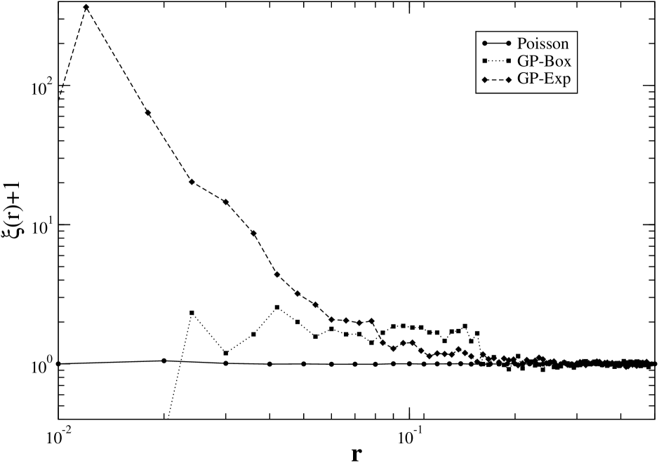
Figure 1: Connected two-points correlation function plus one measured in different types of the particles distribution. The correlations function are taken by averaging over $1000$ realizations of a sample of $N=10^{2}$ particles (in the same fixed volume $V=1$.) Poisson case, the Gauss-Poisson case (GP-box) where $p(r)$ is a $box-function$. and the Gauss-Poisson case (GP-Exp), where $p(r)=\frac{1}{4\pi r_{0}}\frac{\exp(-\frac{r}{r_{0}})}{r^{2}}$.

IV Generalization of the Holtzmark distribution to the Gauss-Poisson case

We can now try to generalize the Holtzmark distribution to this correlated case. Let us suppose of having generated a GP distribution with fixed $n>0$ and $0<q\leq 1$ in a volume $V$ (therefore $N=nV$ with negligible relative fluctuations in different realizations of the distribution in the infinite volume limit). Let us also set the coordinate system in such a way that the origin is occupied by a particle of the system. We want to calculate the PDF $\tilde{W}(\vec{F})$ of the total gravitational field $\vec{F}$ acting on the origin of coordinates due to all the particles out of the origin conditioned to the fact that this point is occupied by a particle of the system . Therefore if the particles seen by the one in the origin are $N-1$ and $p_{c}(\vec{r}_{1},\vec{r}_{2},...,\vec{r}_{N-1})$ is the PDF of their position with respect the origin we can write:

$$\tilde{W}(\vec{F})=\int_{V}...\int_{V}\left[\prod_{i=1}^{N-1}d^{3}r_{i}\right]p_{c}(\vec{r}_{1},\vec{r}_{2},...,\vec{r}_{N-1})\cdot$$ (13)

$$\delta\left(\vec{F}-\sum_{i=1}^{N-1}\frac{\vec{r}_{i}}{r_{i}^{3}}\right)$$

The main problem to face is due to the fact that, since in the GP case, two-points correlations are present, $p_{c}(\vec{r}_{1},\vec{r}_{2},...,\vec{r}_{N-1})$ cannot be written as a product $N-1$ one particle PDF’s as in the Poisson case. This property would prevent from the possibility of applying the Markov method to this case, and an explicit evaluation of $\tilde{W}$ would become impossible. For this reason we introduce the approximation consisting in imposing the factorization

$$p_{c}(\vec{r}_{1},\vec{r}_{2},...,\vec{r}_{N-1})=\prod_{i=1}^{N}\tau(\vec{r}_{i})\,,$$

but taking into account the fact that in average the particle in the origin sees a density of particles in the point $\vec{r}$ given by Eq. 12 with $\xi(\vec{r})=\frac{2q}{n(1+q)}p(\vec{r})$, i.e.

$$\tau(\vec{r})=\frac{1+\frac{2q}{n(1+q)}p(\vec{r})}{V+\frac{2q}{n(1+q)}}\,.$$ (14)

This approximation permits to use the Markov method to find $\tilde{W}(\vec{F})$ which, in the limit $V\rightarrow+\infty$, can be shown to be given by

$$\tilde{W}(\vec{F})=\frac{1}{(2\pi)^{3}}\int d^{3}F\exp\left(i\vec{k}\cdot\vec{F}-nC_{GP}(\vec{k})\right)\,,$$ (15)

where

$$C_{GP}(\vec{k})=C_{P}(k)+\frac{2q}{n(1+q)}\int d^{3}r\,p(\vec{r})\left(1-e^{-i\frac{\vec{k}\cdot\vec{r}}{r^{3}}}\right)\,.$$ (16)

As shown below by a direct comparison with the results of numerical simulations, this approximation is quite accurate at least in the asymptotic regime $F\rightarrow+\infty$. Note that the function $A(\vec{k})=\exp\left(-nC_{GP}(\vec{k})\right)$ is nothing else the characteristic function of the total force $\vec{F}$ acting on the particle in the origin in the GP case. As aforementioned, if the PDF $p(\vec{r})$ depends only on $r=|\vec{r}|$, the particle distribution is statistically isotropic. Consequently, as for the Poisson case, $\tilde{W}(\vec{F})$ also depends only on $F=|\vec{F}|$ and $A(\vec{k})$ on $k=|\vec{k}|$. That is the direction of $\vec{F}$ is completely random while the PDF of $F$ is given by (by recalling $p(\vec{r})$ with $p(r)$ to put in evidence the dependence only on $r$)

$$W(F)\equiv 4\pi F^{2}\tilde{W}(\vec{F})$$ (17)

$$=\frac{2F}{\pi}\int_{0}^{\infty}dkk\sin(kF)\exp\left\{-\frac{4(2\pi)^{\frac{3}{2}}nk^{\frac{3}{2}}}{15}\right.$$

$$-\left.\frac{8\pi q}{1+q}\int_{0}^{\infty}drr^{2}p(r)\left[1-\frac{r^{2}}{k}\sin\left(\frac{k}{r^{2}}\right)\right]\right\}\;.$$

We limit the rest of the discussion to this isotropic case. As for the Poisson distribution, it is not possible to find an explicit form of $\tilde{W}(F)$ (or equivalently of $W(F)$). However we can connect their large $F$ behavior to the small $r$ behavior of $p(r)$ and to that of the Poisson case. In order to do this, it is important to use the general properties of the Taylor expansion of the characteristic function $A(\vec{k})$ to the lowest order greater than zero. In particular in this isotropic case we use that singular , if $\tilde{W}(\vec{F})\sim F^{-\alpha}$ at large $F$ (note that $\alpha>3$ in any case as $\tilde{W}(\vec{F})$ is a normalizable PDF) then

$$A(\vec{k})=\int d^{3}F\exp\left(-i\vec{k}\cdot\vec{F}\right)\tilde{W}(\vec{F})=$$

$$\,=\left\{\begin{array}[]{ll}1-\frac{1}{6}\langle F^{2}\rangle k^{2}&\mbox{ if }\alpha>5\\ 1-ak^{\alpha-3}&\mbox{ if }3<\alpha\leq 5\;,\end{array}\right.$$ (20)

where $a>0$ is a constant characterizing the singularity. Note that $\alpha>5$ implies that $\left<F^{2}\right>$ is finite, and that for the Poisson case $\alpha=9/2$, and correspondingly $A(\vec{k})\simeq 1-\frac{4n}{15}(2\pi k)^{\frac{3}{2}}$.

Therefore our strategy is to find $\alpha$ by connecting the expansion given in Eq. IV to the form of $p(r)$ and in particular to its small $r$ behavior. Let us suppose that $p(r)\sim r^{\beta}$ at small $r$ (in any case $\beta>-3$ as $p(r)$ is a PDF of a three-dimensional stochastic variable). It is quite simple to show that at small $k$ the integral

$$I(k;\beta)=\int_{0}^{\infty}drr^{2}p(r)\left[1-\frac{r^{2}}{k}\sin\left(\frac{k}{r^{2}}\right)\right]$$

behaves as follows:

$$I(k;\beta)\simeq\left\{\begin{array}[]{ll}c_{1}k^{\frac{3+\beta}{2}}&\mbox{if }\beta<1\\ c_{2}k^{2}&\mbox{if }\beta\geq 1\,,\end{array}\right.$$ (21)

where $c_{1}$ and $c_{2}$ are two positive constants depending on the specific form of $p(r)$. Consequently, by inserting this result in Eq. 17, we can distinguish three cases for what concerns the asymptotic behavior of $\tilde{W}(\vec{F})$:

• For $\beta>0$ the dominating part in $A(\vec{k})$ at small $k$ is exactly the same as in the Poisson distribution with the same average density $n$, i.e.

  $$A(\vec{k})\simeq 1-\frac{4n}{15}(2\pi k)^{\frac{3}{2}}\,,$$ (22)

  which implies $\tilde{W}(\vec{F})\sim F^{-\frac{9}{2}}$ (or equivalently $W(F)=4\pi F^{2}\tilde{W}(\vec{F})\sim F^{-\frac{5}{2}}$) at large $F$ with the same amplitude of the pure Poisson case.

• For $\beta=0$ we have again a substantially Poissonian behavior but the coefficient of the non zero order term receives a contribution from two-points correlations:

  $$A(\vec{k})\simeq 1-8\pi n\left(\frac{(2\pi)^{\frac{1}{2}}}{15}+\frac{c_{1}q}{n(1+q)}\right)k^{\frac{3}{2}}\,,$$ (23)

  which implies again $\tilde{W}(\vec{F})\sim F^{-\frac{9}{2}}$ at large $F$ but with a larger amplitude than in the Poisson case.

• for $\beta<0$ the small $k$ behavior of $A(\vec{k})$ is completely changed, being

  $$A(\vec{k})\simeq 1-\frac{8\pi c_{1}q}{1+q}k^{\frac{3+\beta}{2}}\,,$$ (24)

  which gives $\tilde{W}(\vec{F})\sim F^{-\frac{9+\beta}{2}}$ (or equivalently $W(F)=4\pi F^{2}\tilde{W}(\vec{F})\sim F^{-\frac{5+\beta}{2}}$)

V Comparison with simulations

In order to check the validity of these theoretical results, we have performed numerical simulations consisting in generating two kinds of GP distributions of particles with two explicite choices of $p(r)$ (see Fig. 1), and in measuring directly the PDF of $\tilde{W}(\vec{F})$ in these cases:
(1) In the first one the choice of $p(r)$ is simply a positive constant up to a fixed distance $r_{0}$ and zero beyond this distance:

$$p(r)=\left\{\begin{array}[]{ll}\frac{3}{4\pi r_{0}^{3}}&\mbox{if }0<r\leq r_{0}\\ 0&\mbox{if }r<r_{0}\,.\end{array}\right.$$ (25)

That is the probability of attaching a “daughter” particle at a distance between $r$ and $r+dr$ from its “parent” is $3r^{2}dr/r_{0}^{3}$ if $r\leq r_{0}$ and zero for $r>r_{0}$. As shown above this choice of $p(r)$ should give $W(F)\sim F^{-\frac{5}{2}}$ at large $F$ but with a larger amplitude than the pure Poisson case.
(2) In the second case $p(r)$ decays exponentially fast at large $r$ but increases as $r^{-2}$ at small $r$, i.e.

$$p(r)=\frac{1}{4\pi r_{0}}\frac{\exp(-\frac{r}{r_{0}})}{r^{2}}\;\;.$$ (26)

This choice of $p(r)$ should give $W(F)\sim F^{-\frac{3}{2}}$ at large $F$. The results of these simulations for the large $F$ behavior of $\tilde{W}(\vec{F})$ have been compared to the theoretical previsions showing a good agreement (see Fig. 2). Consequently the validity of the approximation at the base of these calculations has been positively tested.

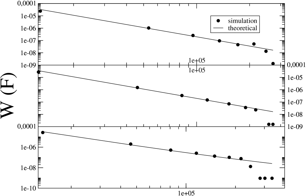
Figure 2: Comparison between theoretical predictions (continuous lines) and simulations of the tail of the probability density function of the modulus of the gravitational force $W(F)=4\pi\tilde{W}(\vec{F})$. The average for the PDF is performed over $2\cdot 10^{4}$ realizations of a the same distribution with each of $N=10^{5}$ particles. Top panel: Poisson case. Middle panel: Gauss-Poisson case, where $p(r)$ is a $box-function$. Bottom panel: Gauss-Poisson case, where $p(r)$ has an exponential cut-off: $p(r)=\frac{1}{4\pi r_{0}}\frac{\exp(-\frac{r}{r_{0}})}{r^{2}}$

The found validity of the relations between the small scale behavior of $\xi(\vec{r})$ and the large scale behavior of $W(F)$ for the GP case suggests that this approach can be extended to more general cases of correlated particle distributions.

VI Nearest Neighbor approximation for the Gauss-Poisson case

As for the Poisson case, we now analyze, for GP distributions in the statistical isotropic case, the importance of the first NN contribution to the total force felt by the particle in the origin. To this aim we use again only the information that the average conditional density $n_{p}(\vec{r})$ (which depends only on $r$) seen by the particle in the origin is given by Eq. 12. Following exactly the same reasoning done for the Poisson case with $n_{p}(\vec{r})$ replacing the simple $n$, we can write:

$$\omega(r)=\left(1-\int^{r}_{0}{\omega(x)dx}\right)4n\pi r^{2}(1+\xi(r))\,,$$ (27)

where again $\xi(r)=\frac{2q}{n(1+q)}p(r)$. Equation 27 can be solved to give

$$\omega(r)=4n\pi r^{2}(1+\xi(r))\exp\left[-4n\pi\int_{0}^{r}s^{2}(1+\xi(s))\right]$$

$$=\omega_{P}(r)+4n\pi r^{2}\exp\left[-4n\pi\int_{0}^{r}s^{2}\xi(s)\right]$$

$$+4n\pi r^{2}\xi(r)\exp\left[-4n\pi\int_{0}^{r}s^{2}(1+\xi(s))\right]\,,$$ (28)

where we have called $\omega_{P}(r)$ the function $\omega(r)$ found above for the Poisson case. By imposing $p(r)\sim r^{\beta}$ at small $r$ and using again $F=1/r^{2}$ in order to pass from $\omega(r)$ to $W_{nn}(F)$, it is simple to see that $W_{nn}(F)$ has the same aforementioned scaling behavior at large $F$ of $W(F)$ for all the permitted values of $\beta$ and with the same coefficient. Therefore also in the GP case we have that the main contribution to the force felt by a particle in the system is due to its first NN. This was somehow expected because the main change introduced by passing from Poisson to GP distribution concerns mainly the introduction of additional fluctuations of density in the neighborhood of any particle.

VII Discussion

In conclusion we have studied the gravitational force distribution in the so called Gauss-Poisson particle distributions, which can be considered in some sense the most weakly correlated case beyond the Poisson one. For this particle systems we have seen how to generalize the methods developed for the Poisson case in order to find the PDF of the gravitational force. The main result is that, in the GP case, significative deviations from the Poisson behavior can be caused only by the small scale behavior of two-points correlations, which can introduce strong modification in the large force regime when diverging at small distances. This is confirmed by direct results in numerical simulations. Moreover, as in the Poisson case, we found that the main contribution to the force felt by a generic particle is due mainly to its neighborhood. The importance of this work is twofold. (i) firstly, this is the first case of statistically homogeneous correlated particle distribution in which a systematic study of the gravitational force à la Chandrasekhar is done, (ii) this study suggest some basic ingredients to be used in future attempts of extending the analysis to more complex correlated particle distributions.

VIII Acknowledgments

We thank L. Pietronero and M. Joyce for useful comments and discussions. A.G. acknowledges the Physics Department of the University “La Sapienza” of Rome (Italy) for supporting this research. F.S.L. acknowledges the support of EC Marie-Curie fellowship HPMF-CT-2001-01443

References

- (1) T. Baertschiger and F. Sylos Labini, Europhys Lett., 57, 322 (2002).
- (2) T. Baertschiger, M. Joyce and F. Sylos Labini, Astrophys.J.Lett, 581, L63 (2002)
- (3) M. Wilkens, Acta Metall., 17, 1155 (1969).
- (4) B.V.Gnedenko, The Theory of Probability, MIR Publishers (Moscow, 1978).
- (5) S.Chandrasekhar, Rev. Mod. Phys., 15, 1 (1943).
- (6) A.Gabrielli, F.Sylos Labini, S.Pellegrini, Europhys. Lett., 46(2), 127 (1999).
- (7) A. Del Popolo, Astron. Astrophys., 311, 715 (1996).
- (8) J.-P. Hansen and I.R. McDonald, Theory of Simple Liquids, Academic Press Limited (London, 1991).
- (9) A. Gabrielli, M. Joyce and F. Sylos Labini, Phys.Rev. D65, 083523 (2002)
- (10) P.Hertz, Math. Ann., 67, 387 (1909).
- (11) D.Stoyan, W.S.Kendall, J.Mecke, Stochastic geometry and its applications, Wiley, (New Yok, 1995).
- (12) M.Kersher, Phys. Rev. E, 64, 056109 (1999).
- (13) D.J.Daley, D.Vere-Jones, An introduction to the theory of point processes, Springer-Verlag (Berlin, 1988).
- (14) B. D. Hughes, Random Walks and Random Environments Vol. 1, Oxford Science Publications (1995).