Polarization of prompt GRB emission:
evidence for electromagnetically dominated outflow

Abstract

Observations by the RHESSI  satellite of large polarization of the prompt $\gamma$-ray emission from the Gamma Ray Burst GRB021206 (Coburn & Boggs, 2003) imply that the magnetic field coherence scale is larger than the size of the visible emitting region, $\sim R/\Gamma$, where $R$ is the radius of the flow, $\Gamma$ is the associated Lorentz factor. Such fields cannot be generated in a causally disconnected, hydrodynamically dominated outflow. Electromagnetic models of GRBs (Lyutikov & Blandford, 2002), in which large scale, dynamically dominant, magnetic fields are present in the outflow from the very beginning, provide a natural explanation of this large reported linear polarization. We derive Stokes parameters of synchrotron emission of a relativistically moving plasma with a given magnetic field configuration and calculate the pulse averaged polarization fraction of the emission from a relativistically expanding shell carrying global toroidal magnetic field. For viewing angles larger than $1/\Gamma$ the observed patch of the emitting shell has almost homogeneous magnetic field, producing a large fractional polarization ($56\%$ for a power-law energy distribution of relativistic particles $dn/d\epsilon\propto\epsilon^{-3}$). The maximum polarization is smaller than the theoretical upper limit for a stationary plasma in uniform magnetic field due to relativistic kinematic effects.

1 Introduction

Origin of magnetic fields in Gamma Ray Bursts (GRBs) is one of the central unresolved issues. In the standard fireball scenario (e.g. Piran 1999, Mészáros 2002 and references therein), magnetic field does not play any dynamical role. The near-equipartition field invoked in the emission region is assumed to be generated locally at relativistic shocks by plasma instabilities (e.g. Medvedev & Loeb 1999). Initially, the spatial scale of such fields is microscopically small, of the order of the ion skip depth, $\delta\sim c/\omega_{p,i}$ ($\omega_{p,i}$ is the ion plasma frequency). Though the typical scale of magnetic field fluctuations may grow due to inverse cascade, even in the unlikely case that such growth proceeds at the speed of light the resulting polarization is expected to be smaller than $10\%$ (e.g.  Gruzinov & Waxman, 1999).

The recent detection by the RHESSI  satellite of large polarization in the prompt $\gamma$-ray emission (Coburn & Boggs, 2003) places severe constraints on the GRB models. It implies that magnetic field coherence scale is larger than the size of the visible emitting region, $\sim R/\Gamma$, where $R$ is the distance form the center and $\Gamma$ is a bulk Lorentz factor of relativistically expanding emission region. Such fields cannot be generated in a hydrodynamically dominated outflow, which is causally disconnected on large scales. Thus, the large scale magnetic fields should be present in the outflow from the very beginning. In fact, as we argue below, such fields must be dynamically dominant, carrying most of the energy of the outflow.

Building upon earlier models of electromagnetic explosions (e.g.  Usov, 1992; Thompson, 1994; Smolsky & Usov, 1996; Mészáros & Rees, 1997), Lyutikov & Blandford (2002, 2003) developed an electromagnetic model of GRBs which assumes that rotating, relativistic, stellar mass progenitor (e.g. “millisecond magnetar”, Usov 1992) loses much of its spin energy in the form of an electromagnetically dominated outflow. A stellar mass relativistic progenitor is born with angular velocity $\Omega\sim 10^{4}$ s^-1 and dynamo generated magnetic field of $B_{\rm s}\sim 3\times 10^{14}$ G. Then the total rotational energy, $E\sim I\Omega^{2}/2\sim 5\times 10^{52}$ erg (for a $1.4\,M_{\odot}$ object) is available to power GRB bursts, while the dipole spin-down luminosity $L_{P}\simeq{B_{\rm s}^{2}r_{s}^{6}\Omega^{4}/c^{3}}\simeq 10^{49}\,{\rm ergss^{-1}}$ is about the luminosities of cosmological $\gamma$-ray bursters. In this model the energy to power the GRBs comes eventually from the rotational energy of the progenitor. It is first converted into magnetic energy by the dynamo action of the unipolar inductor, propagated in the form of Poynting flux dominated flow and then dissipated at large distances from the sources.

A rapidly spinning magnetar with a complicated field structure will form a relativistic outflow. We suggest that magnetic field in the wind quickly rearrange to become predominantly axisymmetric. There is a good precedent for this behavior in Ulysses observations of the quiet solar wind (McComas et al. , 2000) which reveal that, despite the complexity of the measured surface magnetic field, the field in the solar wind quickly rearranges to form a good approximation to a Parker (1960) spiral. The situation in the far field will then resemble that first analyzed by Goldreich & Julian (1969) and the characteristic scale length in the far field is the cylindrical radius from a polar axis, rather than the wavelength.

During the relativistic expansion, most of the magnetic energy carried by axisymmetric toroidal magnetic fields is concentrated in a thin shell with thickness $\Delta r\sim ct_{s}\sim 3\times 10^{12}$ cm inside a contact discontinuity separating the ejecta from the shocked circumstellar material. At the contact discontinuity toroidal magnetic field balances the ram pressure of the circumstellar material $B_{\phi}\sim 4\Gamma^{2}\sqrt{\pi\rho_{\rm ext}c^{2}}$. Both $B_{\phi}$ and $\Gamma$ depend on the angle between a given point on the shell and the polar axis, defined as the axis of rotation of the progenitor. This results in a non-spherical, relativistic expansion of the shell. In particular, for laterally balanced expansion $\Gamma\sim 1/\sin\theta$. The current carrying shell becomes unstable due to development of the current driven instabilities at a radius $\sim 10^{16}$ cm. This leads to acceleration of pairs which emit $\gamma$-rays by synchrotron radiation.

A distinctive feature of the electromagnetic model is that the causal connection is better than in the hydrodynamic models. Initially, close to the central source the subsonic flow is fully causally connected. As the flow is accelerated by magnetic (and partially by pressure) forces it becomes supersonic, strongly relativistic and causally disconnected over small polar angles $\Delta\theta\sim 1/\Gamma$. Later, magnetically dominated flows quickly reestablish causal contact over large polar angles and become fully causally-connected again after a time $t_{\rm c}\sim t_{s}\Gamma^{2}$, where $t_{s}\sim 100$ sec is the source activity life time. This is drastically different from hydrodynamic flows which remain causally disconnected over polar angles larger than $1/\Gamma$. Thus, during expansion the causal behavior of the flow resembles the behavior of cosmic fluctuations during inflation: as the flow expands, angular scales $\sim\Gamma^{-1}$ “enter the horizon” re-establishing causal contact that was lost during acceleration.

To illustrate this behavior, consider propagation of a sound-type disturbance emitted by a point source located on the relativistically moving shell at radius $R_{\rm em}$. Let the typical signal speed in the plasma rest frame be $\beta_{s}$. In appendix A we show that for sub-Alfvenic ejecta (magnetically dominated flows can be strongly relativistic, but still sub-Alfvenic!) a relativistically expanding shell re-establishes a causal contact over the visible patch of $1/\Gamma$ in just one dynamical time scale (after doubling in radius). If the ratio of the magnetic to particle energy density in the cold, magnetized plasma is $\sigma=u_{B}/u_{\rm p}\gg 1$ (Kennel & Coroniti, 1984), then the Alfvén (and fast magneto-sound) velocity is $\beta_{\rm A}=c\sqrt{\sigma/(1+\sigma)}$. The requirement that the expansion velocity be sub-Alfvenic then implies that $c\Gamma\leq u_{\rm A}$ or $\sigma\gg 1$. Therefore, the condition that magnetic fields have a coherence scale larger than $R/\Gamma$ requires that the magnetic fields be energetically dominant in the flow.

Hydrodynamic (e.g. fireballs, Piran 1999, or external shocks, Dermer 2002, with $\sigma\ll 1$) or hydromagnetic models ($\sigma\sim 1$, e.g. Spruit et al.  2000, Drenkhahn & Spruit 2002, Vlahakis & Königl 2003) could also have a large scale ordered magnetic field (cannonballs, e.g. Dar 2003, need to rely on energetically inefficient Compton scattering and strong flow inhomogeneities on the angular scale $\sim 1/\Gamma$, Coburn & Boggs (2003), section 3; we consider this prohibitively tight constraints). In all cases, the whole outflow is in causal contact close to the source and may have a large scale magnetic field which will be carried with the flow. In hydro-dominated models, after the causal contact is lost, different parts of the flow cannot communicate and thus will evolve differently, depending on the local conditions. Only under strict homogeneity of the surrounding medium and of the ejecta the two causally disconnected parts of the flow will have similar properties. On the other hand, since magnetically dominated outflows can quickly communicate information (e.g. magnetic pressure) over large polar angles, they can have quasi-homogeneous properties despite possible inhomogeneities in the circumstellar medium and in ejecta.

Assumption of electromagnetically dominated flow must eventually break down, since the ejecta need to dissipate magnetic energy to produce high energy emission. In the emission region the plasma is expected to be close to equipartition as magnetic field is dissipated to accelerate electrons (generally, equipartition is needed for effective emission). But unlike the hydrodynamic models where equipartition is reached by amplifying weak magnetic fields at the shocks, in the electromagnetically dominated model the equipartition is reached by dissipation of initially dominant magnetic field, as, for example, happens in solar flares.

In this paper we calculate the Stokes parameters for the prompt GRB emission emerging in electromagnetic model as a function of the viewing angle (angle between the line of sight and the polar axis of the flow). We assume that magnetic field in the emission region is dominated by the toroidal field and is concentrated in a thin shell $\Delta R$ near the surface of the shell expanding with the Lorentz factor $\Gamma(\theta)$. Synchrotron emission is produced by an isotropic population of relativistic electrons with the power law distribution in energy. In the present work we calculate Stokes parameters averaged over the duration of the GRB pulse, deferring the time-dependent calculations to a later work. One expects that the polarization fraction will be maximal in the beginning of the pulse, slightly decreasing towards the end as larger emitting volumes become visible. We set the speed of light to unity, $c=1$, in all the expressions to follow.

2 Calculation of Stokes parameters

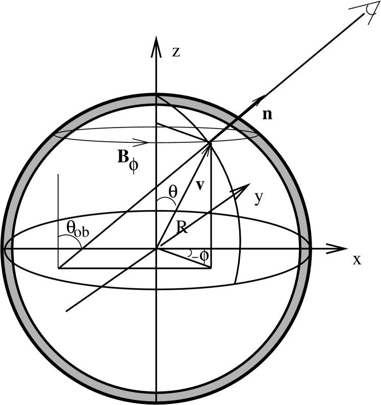
Figure 1: Geometry of the model. A narrow shell $\Delta r\sim t_{s}c\sim 3\times 10^{12}$ cm, dominated by the toroidal magnetic field, expands quasi-spherically with angle dependent velocity ${\bf v}(\theta)$. The observer is located at an angle $\theta_{\rm ob}$ with respect to the polar axis.

Consider a quasi-spherical thin emitting shell (Fig. 1) viewed by an observer. Below we denote all quantities measured in the local frame comoving with an emitting elementary volume with primes, while unprimed notations refer to the quantities measured in the explosion frame. Let $r$, $\theta$, and $\phi$ be the spherical coordinates in the coordinate system centered at the center of the shell, and $x$, $y$, and $z$ be the rectangular coordinates with the origin at the center of the shell. The symmetry axis of the shell is the $z$-axis. The toroidal magnetic field in the shell is in the $\phi$-direction. The observer is located in the $x$–$z$ plane. The components of all vectors written below are the components with respect to the rectangular coordinate system $x$, $y$, and $z$. The shell expands quasi-spherically with an angle-dependent Lorentz factor $\Gamma(\theta)$. An element of the shell moving radially with the velocity ${\bf v}=\beta\{\sin\theta\cos\phi,\sin\theta\sin\phi,\cos\theta\}$ emits a burst of synchrotron radiation in the direction of unit vector ${\bf n}=\{\sin\theta_{\rm ob},0,\cos\theta_{\rm ob}\}$ when viewed in the observer frame.

Several key ingredients need to be taken into account (e.g. Cocke & Holm 1972, Blandford & Königl 1979, Bjornsson 1982, Ginzburg 1989). First, the synchrotron emissivity depends on the direction between the emitted photon and the magnetic field in the plasma rest frame. Second, as the emission is boosted by relativistic motion of the shell, the position angle of the linear polarization rotates in the ${\bf n}-{\bf v}$ plane. The fractional polarization emitted by each element remains the same, but the direction of polarization vector of the radiation emitted by different elements within a visible shell is rotated by different amounts. This leads to effective depolarization of the total emission. The theoretical maximum polarization fraction for homogeneous field can be achieved only for uniform plane-parallel velocity field. Third, integration along the line of sight (and over the emitting solid angle for unresolved sources) is better carried out in the laboratory frame, in order to take correct account of the arriving times of photons.

We assume that the distribution function of emitting particles in the frame comoving with an element of the shell is isotropic in momentum and is a power law in energy

$$dn=K_{\rm e}\epsilon^{-p}d\epsilon dVd\Omega_{\bf p}\mbox{.}$$ (1)

Here $dn$ is the number of particles in the energy interval $\epsilon,\epsilon+d\epsilon$, $dV$ is the elementary volume, $d\Omega_{\bf p}$ is the elementary solid angle in the direction of the particle momentum ${\bf p}$, $K_{\rm e}=K_{\rm e}(r)$, $p={\rm constant}$.

In this paper we are interested in the polarization structure of the time integrated pulse of the emission, and not in its temporal properties. Hence, for simplicity we approximate the $\gamma$-ray emissivity of the shell as a flash at some time $t_{0}$ in the explosion frame, lasting for $\Delta t\ll\Delta R/c$, where $\Delta R\ll R_{0}$ is the thickness of the shell at the moment $t_{0}$ and $R_{0}$ is the radius of the shell at the moment $t_{0}$. More complicated emission profiles may be easily accommodated. In addition, we integrate over the observer time to get an average polarization of the pulse deferring time dependent calculations to a later work.

We also assume that the emission is optically thin and neglect possible plasma propagation effects (e.g., depolarization of radiation due to internal Faraday rotation by low energy electrons). Since the emitting particles are ultra-relativistic and we neglect conversion of linear to circular polarization in plasma, we do not have circular polarization in our model (Stokes $V=0$). We also neglect a possible tangled component of the magnetic field present in the emission region. We assume that the emission originates in a geometrically thin layer $\Delta R\ll R$ with the thickness $\Delta R$ independent on $\theta$ and neglect variation of the magnetic field and velocity across the layer. Given these assumptions, our estimates provide an upper limit on the possible polarization.

Time-integrated Stokes parameters are calculated in appendix B (Eqns. (B7)). Due to cylindrical symmetry of the model the Stokes parameter ${\bar{U}}$ integrates to zero, so that the observed averaged polarization fraction is

$${{\Pi}}={|{\bar{Q}}|\over{\bar{I}}}=\frac{p+1}{p+7/3}{\int\sin\theta d\theta d\phi\,{\cal D}^{2+(p-1)/2}|B^{\prime}\sin\chi^{\prime}|^{(p+1)/2}\cos 2{\tilde{\chi}}\over\int\sin\theta d\theta d\phi\,{\cal D}^{2+(p-1)/2}|B^{\prime}\sin\chi^{\prime}|^{(p+1)/2}}\mbox{.}$$ (2)

Here $B^{\prime}$ is the magnitude of the magnetic field ${\bf B}^{\prime}$ in the frame of an element of the shell, $\chi^{\prime}$ is the angle that the line of sight in the frame of an element of the shell, ${\bf n}^{\prime}$, makes with the magnetic field ${\bf B}^{\prime}$, and $\tilde{\chi}$ is the position angle of the electric field vector in the observer plane of the sky measured from some reference direction. Doppler boosting factor is ${\cal D}={1/\Gamma(1-{\bf n}\cdot{\bf v})}\mbox{.}$ For toroidal magnetic field ${\bar{Q}}>0$, so that the observed polarization vector is always along the projection of the flow axis on the plane of the sky.

Evaluation of different quantities in Eqn. (2) is an involved exercise in Lorentz transformations. We assume that, in the shell frame, the magnetic field is purely toroidal

$${\bf B}^{\prime}=b_{\phi}(r,\theta)\hat{{\bf B}}^{\prime}=b_{\phi}\{-\sin\phi,\cos\phi,0\}\mbox{,}$$ (3)

where $\hat{{\bf B}}^{\prime}$ is the unit vector along ${\bf B}^{\prime}$ in the radiating element frame and $b_{\phi}$ is the magnitude of the field. A photon propagating along the unit vector ${\bf n}$ in the explosion frame is emitted along the direction with the unit vector ${\bf n}^{\prime}$ in the radiating element frame:

$${\bf n}^{\prime}=\frac{{\bf n}+\Gamma{\bf v}\left({\Gamma\over\Gamma+1}({\bf n}\cdot{\bf v})-1\right)}{\Gamma\left(1-({\bf n}\cdot{\bf v})\right)}\mbox{.}$$ (4)

Note, that ${\bf n}^{\prime},{\bf n}$ and ${\bf v}$ lie in the same plane. The angle $\chi^{\prime}$ between the photon and magnetic field in the radiating element frame is

$$\cos\chi^{\prime}={\hat{{\bf B}}^{\prime}\cdot{\bf n}^{\prime}}={(\hat{{\bf B}}^{\prime}\cdot{\bf n})+\Gamma(\hat{{\bf B}}^{\prime}\cdot{\bf v})\left({\Gamma\over\Gamma+1}({\bf n}\cdot{\bf v})-1\right)\over\Gamma(1-({\bf n}\cdot{\bf v}))}$$ (5)

which gives

$$\sin^{2}\chi^{\prime}=1-\frac{\sin^{2}\phi\sin\theta^{2}_{\rm ob}}{\Gamma^{2}(1-\beta\mu)^{2}}\mbox{,}$$ (6)

where $\mu=\cos\theta\cos\theta_{\rm ob}+\sin\theta\sin\theta_{\rm ob}\cos\phi$.

We also need to evaluate angle $\tilde{\chi}$ between a given direction in the observer plane and the polarization vector. This is not trivial since polarization vector emitted by each element will experience rotation during Lorentz transformation from the shell frame to the laboratory frame (Cocke & Holm, 1972; Blandford & Königl, 1979). Rotation of the polarization vector is due to the rotation of the wave vector in the plane containing vectors ${\bf n}$, ${\bf n}^{\prime}$, and ${\bf v}$, and the requirement that the electric field of the wave remains orthogonal to the wave vector. Since wave vectors of emitted waves experience rotation by angles of the order of unity, this effect would lead to effective depolarization of emission from a medium with non-uniform velocity field even from a homogeneous magnetic field. In appendix C we derive general relations for the Lorentz transformation of the polarization vector.

We choose to measure angle $\tilde{\chi}$ clockwise from the direction parallel to the projection of the axis of the flow on the plane of the sky. The unit vector in this direction is $\{-\cos\theta_{\rm ob},0,\sin\theta_{\rm ob}\}$. We find (appendix C)

$$\cos\tilde{\chi}={(1-\beta\mu)\cos\phi-\beta\sin\theta\sin\theta_{\rm ob}\sin^{2}\phi\over\sqrt{(1-\beta\mu)^{2}-\sin^{2}\theta_{\rm ob}\sin^{2}\phi/\Gamma^{2}}}\mbox{,}\mbox{}$$

$$\sin{\tilde{\chi}}=\frac{\sin\phi(\beta\cos\theta-\cos\theta_{\rm ob})}{\sqrt{(1-\beta\mu)^{2}-\sin^{2}\theta_{\rm ob}\sin^{2}\phi/\Gamma^{2}}}\mbox{.}$$ (7)

In the ultra-relativistic limit, $\Gamma\gg 1$, general relations simplify and it becomes possible to determine analytically the maximum polarization fraction for a given velocity field in the limit $\theta_{\rm ob}\Gamma\gg 1$ (appendix D). For $p=3$ we find $\Pi=9/16$, in excellent agreement with numerical calculations.

On Fig. 2 we plot the map of the polarized emissivity from the shell moving with a constant $\Gamma$ and with constant $b_{\phi}$ as it is seen by the observer on the plane of the sky. $l$ and $s$ are rectangular coordinates on the plane of the sky centered at the projection of the center of the shell. Axis $s$ is directed parallel to the projection of the axis of the shell on the sky. $l$ and $s$ are normalized such that the projection of the shell radius, $R_{s}$, is a circle of radius $1$ in the $l$–$s$ plane. Thus,

$$l=\frac{1}{R_{s}}{\bf l}\cdot{\bf r}=\sin\theta\cos\phi\mbox{,}\,\,\,s=-\frac{1}{R_{s}}{\bf r}\cdot({\bf l}\times{\bf n})=-\cos\theta_{\rm ob}\sin\theta\cos\phi+\sin\theta_{\rm ob}\cos\theta\mbox{,}$$

where ${\bf l}=\{0,1,0\}$ is the unit vector along $l$. The arrows on the plots in Fig. 2 are directed perpendicular to the unit vector in the direction of the electric field of the wave, ${\hat{\bf e}}$, so that in the non-relativistic limit, $\Gamma\to 1$, the arrows are aligned with the magnetic field ${\bf B}$. The length of the arrows is proportional to the synchrotron emissivity from the unit volume, i.e., to the expression under the integral for ${\bar{I}}$ in Eq. (B7). Actual observed intensity is modified by the geometric factor proportional to the path of the ray inside the volume of the shell. For $R_{s}-r\gg\Delta R$, the geometric factor is $1/\mu$. For $\Gamma\gg 1$, Doppler boosting leads to the small effective emitting area of the shell: $l\leq 1/\Gamma$ and $s\leq 1/\Gamma$. Relativistic swing of polarization vector is also clearly visible in Fig. 2. Each patch of the shell emits radiation with the same polarization degree, $\Pi_{\rm max}=(p+1)/(p+7/3)$. Due to summation over the areas of the shell with different directions of $\tilde{\chi}$, resulting polarization degree becomes smaller than $\Pi_{\rm max}$.

We are now in a position to estimate polarization fraction (2) integrating Stokes parameters (B7) over an expanding relativistic shell. Results for ${\Pi}$ are shown in Fig. 3. The parameter ${\bar{Q}}$ is zero for $\theta_{\rm ob}=0$ and is small for $\theta_{\rm ob}<1/\Gamma$, because the polar axis falls within the visible patch in this case. The magnetic field changes its direction within the visible patch and the resulting polarization is reduced. The degree of polarization reaches a limiting value of tens percent when observation angle is larger than $1/\Gamma$.

3 Discussion

Large scale ordered magnetic fields produced at the central source provide a simple explanation of the recent observations of highly polarized GRB prompt emission by the RHESSI  satellite (Coburn & Boggs, 2003). In order to retain the coherence of the magnetic field on scales larger than the visible patch, $\sim R/\Gamma$, the ejecta must be electromagnetically dominated. The electromagnetic model suggested by Lyutikov & Blandford (2002, 2003) provides a solution to the puzzle of how to produce large coherent magnetic fields and how to launch a blast wave that extends over an angular scale $>>\Gamma^{-1}$ and where the individual parts are out of causal contact. In the electromagnetic model, the magnetic fields are present in the outflow from the very beginning, and the energy is transferred to the blast wave by a magnetic shell which is causally connected at the end of the coasting phase.

To prove this point we first found general relations for transformation of polarization direction of synchrotron emission produced by relativistically moving source with a given magnetic field structure and calculated Stokes parameters for the time averaged synchrotron emission for a particular case of relativistically expanding shell containing toroidal magnetic fields. We find that for observing angles satisfying $\theta_{\rm ob}\geq 1/\Gamma$ a large polarization fraction $\Pi\sim 60\%$ may be observed (the actual spectrum was not measured for GRB021206). The position angle of the polarization is fixed by the projection of the progenitor axis on the plane of the sky and thus should not change during the burst.

Another potential source of polarization could be Compton scattering of unpolarized $\gamma$-rays. If unpolarized $\gamma$-rays are initially beamed into a small-angle jet and are scattered by surrounding gas, then polarized scattered $\gamma$-rays would be distributed nearly isotropically. This will require a much higher energy in the initial $\gamma$-ray jet than the energy necessary if the narrowly beamed jet is observed directly (Coburn & Boggs, 2003), thus putting a much tougher requirement for the total energy budget of GRB. Compton scattering by relativistically moving wide angle envelope could also occur. In this case kinematics of the scattering is similar to the kinematics of the synchrotron emission considered in the present work. Therefore, the energetic requirements are also similar to the synchrotron mechanism. However, Compton scattered photons do not have preferred direction of polarization, which is set by the large scale magnetic field in the synchrotron case. The net polarization of scattered photons from uniform spherical shell averages to zero. High polarization can be observed only if the shell parameters ($\Gamma$ or electron density) vary significantly on the angular scale $\sim 1/\Gamma$. We are coming back to highly collimated flow. Therefore, we conclude that Compton scattering cannot account for the high degree of polarization of $\gamma$-rays emerging from a wide angle expanding flow. We note, that synchrotron mechanism results in the electric vector of polarized emission directed parallel to the axis of the flow, while the scattered $\gamma$-rays would be polarized in the direction perpendicular to the axis of flow.

Several natural correlations between GRB polarization and other parameters follow from the model and can be tested with future observations. First, polarization fraction should decrease from the beginning to end of the pulse as larger areas of the emitting shell become visible to the observer. Second, the maximum amount of polarization is related to the spectrum of emitting particles, being higher for softer spectra. This points to a possible correlation between the amount of polarization and hardness of the spectrum.

Our treatment of the prompt emission may also be related to polarization of afterglows. If the field from the magnetic shell may be mixed in with the shocked circumstellar material (similar to the so called flux transfer events at the day side of Earth magnetosphere), then a comparably large fractional polarization may be observed in afterglows as well. In addition, since the preferred direction of polarization is always aligned with the flow axis, the position angle should not be changing through the afterglow (if polarization is observed both in prompt and afterglow emission the position angle should be the same). Also, polarization should not be related to the ”jet break” moment. This is in a stark contrast with the jet model, in which polarization is seen only near the ”jet break” times and the position angle is predicted to experience a flip during the ”jet break” (Sari, 1999). For the same reason large average polarization cannot be due to particular viewing geometry, as suggested by Waxman (2003). Current polarization data show that in virtually all cases position angle remains constant (Covino et al. 2003a, b; Barth et al.  2003; Bersier et al.  2003, see though Rol et al.  2003), while the amount of polarization does not show any correlation with the ”jet break”. This is consistent with the presence of large scale ordered magnetic fields in the afterglows. (A model of Rossi et al.  (2002) of structured jets also predicts constant position angle, but since no large scale magnetic field is assumed the polarization features are still related to the jet break times).

In our calculations we have neglected a random component of the magnetic field which must be present in the emission region. Lyutikov & Blandford (2002, 2003) suggested that $\gamma$-ray emitting electrons are accelerated by current instabilities, somewhat similar to solar flares. Development of current instabilities should be accompanied by dissipation of magnetic fields and destruction of the magnetic flux. These will generally add a random component to the ordered magnetic field and will lead to a decrease in polarization (Korchakov & Syrovatskii, 1962). The corresponding calculations are in progress.

An alternative model of GRBs that can feasibly give large scale magnetic fields in the prompt emission region is the plerion model (Königl & Granot 2002; Inoue et al.  2003, see also Lyutikov 2002), which initially was suggested for afterglows, but may also be extended to include the prompt emission by external shock wave (Dermer, 2002). In this case, the large scale equipartition magnetic fields are created ahead of the expanding GRB ejecta by the preceding explosion of the “supranova” (Vietri & Stella, 1999). Still this type of models faces similar causality/efficiency problem: if the plerion plasma is only at equipartition, $\sigma\sim 1$, it may be expected to be inhomogeneous on $R/\Gamma$ scale; if it is strongly magnetized, $\sigma\gg 1$, then the shocks will be only weakly dissipative.

Implications of the RHESSI  results, that GRB flows are electromagnetically-driven, may provide an important clue to the dynamics of other astrophysical sources like pulsars, (micro)quasars and AGNs. It is quite plausible that all these sources produce ultra-relativistic magnetically dominated outflows with low baryon density (Blandford, 2002). The flow evolution in all these systems may proceed in a similar way. Energy, transported primarily by magnetic fields, is dissipated far away from the source due to development of current instabilities. Particles are accelerated in localized current sheets by DC electric fields and/or electromagnetic turbulence producing bright knots (in AGNs) and a variety of bright spots in pulsar jet, best observed in the Crab.

Appendix A Causal structure of relativistic magnetized outflows

In this appendix we consider the casual structure of the relativistically expanding magnetized shell. We wish to answer the question: ”If a surface of relativistically expanding magnetized shell is perturbed at a given radius $R_{\rm em}$ and zero polar angle, which points on the surface of the shell will be affected after time $t$”.

Consider propagation of a sound-type disturbance emitted by a point source located on the surface of relativistically moving shell at radius $R_{\rm em}$. Let the signal speed in the plasma rest frame be $\beta_{s}$. For simplicity we assume that the shell is moving with constant velocity. If in the plasma frame a wave is emitted in the direction $\theta_{\rm em}$ with respect to the flow velocity, then in the laboratory frame the components of the wave velocity along and normal to the bulk velocity are

$$\beta_{s,lab,\parallel}={\beta+\beta_{s}\cos\theta_{\rm em}\over 1+\beta\beta_{s}\cos\theta_{\rm em}},\,\,\,\beta_{s,lab,\perp}={\beta_{s}\sin\theta_{\rm em}\over\Gamma(1+\beta\beta_{s}\cos\theta_{\rm em})}\mbox{.}$$ (A1)

The condition that a waves catches the surface of the shell becomes

$$(R_{\rm em}+t\beta)\sin\theta={t\beta_{s}\sin\theta_{\rm em}\over\Gamma(1+\beta\beta_{s}\cos\theta_{\rm em})}\mbox{,}\mbox{}$$

$$(R_{\rm em}+t\beta)\cos\theta=R_{\rm em}+{\beta+\beta_{s}\cos\theta_{\rm em}\over 1+\beta\beta_{s}\cos\theta_{\rm em}}t\mbox{.}$$ (A2)

Eliminating $\theta_{\rm em}$ we find

$$2(\beta\,\Gamma)^{2}(1-\beta_{s}^{2})\sin^{2}{\theta\over 2}=\sqrt{1-{\beta(2R_{\rm em}+\beta t)\beta_{s}^{2}\over(R_{\rm em}+\beta t)^{2}}}+{\beta\beta_{s}^{2}\over R_{\rm em}+\beta t}t-1\mbox{.}$$ (A3)

In case of isotropic relativistic fluid with internal sound speed $\beta_{s}=1/\sqrt{3}$, Eq. (A3) implies that the maximum angle that sound waves can reach as $t\rightarrow\infty$ is $\theta\sim\sqrt{\sqrt{6}-2}/\gamma\sim 0.67/\gamma$. Thus, hydro-dominated relativistic plasma remains causally disconnected on scales $\theta\sim 1/\Gamma$ at all times.

In magnetically dominated medium the situation is drastically different. Consider, for simplicity, cold magnetically dominated plasma. If the ratio of the magnetic to particle energy density in the flow is $\sigma=u_{B}/u_{\rm p}\gg 1$ (Kennel & Coroniti, 1984), the Alfvén velocity is $\beta_{\rm A}=\sqrt{\sigma/(1+\sigma)}$. Eq. (A3) then becomes

$$2(\beta\,\Gamma)^{2}\sin^{2}{\theta\over 2}=\sqrt{(1+\sigma)\left(1+{R_{\rm em}^{2}\sigma\over(R_{\rm em}+\beta t)^{2}}\right)}-\left(1+{R_{\rm em}\sigma\over R_{\rm em}+\beta t}\right)\mbox{.}$$ (A4)

This implies that two points on the surface of the shell separated by an angle $\theta\ll 1$ come into causal contact after time

$${ct\over R_{\rm em}}\sim\Gamma\theta\sqrt{1+\sigma\over\sigma}\mbox{.}$$ (A5)

Thus, in strongly magnetized medium, $\sigma\gg 1$, the visible patch of the shell with $\theta\sim 1/\Gamma$ re-establishes causal contact in one dynamical time $t\sim R_{\rm em}/c$.

We may also invert Eq. (A4) to find time needed to establish casual contact over angle $\theta$:

$$t={2R_{\rm em}\beta\,\Gamma\sin{\theta\over 2}\over\beta\left(\sigma-4(\beta\,\Gamma)^{2}\sin^{2}{\theta\over 2}(1+(\beta\,\Gamma)^{2}\sin^{2}{\theta\over 2})\right)}\mbox{,}\mbox{}$$

$$\times\left(\sqrt{\sigma(1+\sigma)(1+(\beta\,\Gamma)^{2}\sin^{2}{\theta\over 2})}+\beta\,\Gamma\sin{\theta\over 2}\left(\beta\,\Gamma+2(1+(\beta\,\Gamma)^{2}\sin^{2}{\theta\over 2})\right)\right)\mbox{.}$$ (A6)

For $\sigma<4\Gamma^{2}(1+\Gamma^{2})$ the maximum causally connected region (for $t\rightarrow\infty$) is finite

$$\sin^{2}{\theta_{\infty}\over 2}={\sqrt{1+\sigma}-1\over 2(\beta\,\Gamma)^{2}}\mbox{.}$$ (A7)

For subsonic flow, $\sqrt{\sigma}>\Gamma$, $\theta_{\infty}$ becomes larger than $1/\Gamma$. For larger $\sigma$ whole shell comes into a causal contact after time

$$t={2R_{\rm em}\beta\,\Gamma\over\beta(\sigma-4\Gamma^{2}(1+\Gamma^{2}))}\left(2(\beta\,\Gamma)^{3}+\sqrt{\sigma(1+\sigma)(1+(\beta\,\Gamma)^{2})}+\beta\,\Gamma(2+\sigma)\right)\mbox{.}$$ (A8)

It is also instructive to find the emission angle $\theta_{\rm em}$ as a function of time $t$ when an emitted wave catches with the surface of the shell:

$$\cos\theta_{\rm em}=-{1\over\beta\beta_{s}(2R_{\rm em}+\beta t)}\left((R_{\rm em}+\beta t)-\sqrt{(R_{\rm em}+\beta t)^{2}-t\beta(2R_{\rm em}+\beta t)\beta_{s}^{2}}\right)\mbox{.}$$ (A9)

In an ultra-magnetized plasma (force-free plasma, $\sigma\rightarrow\infty$) relations simplify considerably. The region casually connected after time $t$ becomes

$$\sin{\theta\over 2}={1\over 2\Gamma}\sqrt{t^{2}\over R_{\rm em}(R_{\rm em}+\beta t)}\mbox{,}\mbox{}$$

$$t=2R_{\rm em}\Gamma\sin{\theta\over 2}\left(\beta\,\Gamma\sin{\theta\over 2}+\sqrt{1+(\beta\,\Gamma)^{2}\sin^{2}{\theta\over 2}}\right)\mbox{.}$$ (A10)

So that points separated by $1/\Gamma$ come into causal contact after $t=(1+\sqrt{5})R_{\rm em}/2$ and the whole shell becomes causally connected after $t\sim 2R_{\rm em}\Gamma^{2}$. Emission angle (A9) in the force-free case then becomes

$$\cos\theta_{\rm em}=-{t\over 2R_{\rm em}+t\beta}\mbox{.}$$ (A11)

Note that in the plasma rest frame the waves which propagate furthermost in polar angles are emitted “backward” in the explosion frame. It is due to this fact why they can “beat” the commonly called result that lateral velocity in the laboratory frame cannot be larger than $c/\Gamma$. The latter is true only for waves propagating along the surface of the shell (normal to the flow in the shell frame). We can understand then why hydrodynamic sound waves cannot reach large polar angles: when emitted “backward”, they are advected with the supersonically moving flow. On the other hand, in subsonic strongly magnetized plasma fast magnetosound waves can outrun the flow and reach large polar angles in the laboratory frame.

Thus, if the effective signal velocity ( Alfvén velocity) in the bulk of the flow is larger than the expansion velocity, strongly relativistic magnetized outflows quickly become casually re-connected over the visible patch $\Delta\theta\sim 1/\Gamma$. For strongly subsonic flows, $\sigma\gg\Gamma^{2}$, points on the shell separated by $1/\Gamma$ come into causal contact on a dynamical time scale $t\sim R_{\rm em}$ (in a relativistic hydrodynamical flow this never happens). Since this time is fairly short, the global dynamics of the flow is not very important which vindicates our assumption of constant expansion velocity.

Appendix B Pulse-integrated Stokes parameters

The Stokes parameters are components of the polarization tensor $J_{ls}=\frac{1}{2}\left(\begin{array}[]{cc}I+Q&U\\ U&I-Q\end{array}\right).$ Here $x_{l}$ are coordinates in the plane perpendicular to ${\bf n}$ and there is no circular polarization. The pulse-integrated intensity

$${\bar{J}}_{ls}(\nu)=\frac{1}{D^{2}}\int\,dT\int dVj_{ls}\left({\bf n},\nu,{\bf r},T+\frac{r\cos\Theta}{c}\right)\mbox{.}$$ (B1)

where $j_{ls}$ is emissivity, $T=t-r\cos\Theta/c$ is the observer time and integration is over the whole emitting region in the explosion frame.

We approximate emissivity as an instant flash at the moment $t=t_{0}$ with the duration $\Delta t$, $\Delta t\ll\Delta R/c$. We also assume that the whole shell emits uniformly during the flash. Then, the emissivity can be expressed as

$$j_{ls}({\bf n},\nu,{\bf r},t)=j_{ls}({\bf n},\nu,t_{0})\delta(t-t_{0})\Delta t\left[H(r-R_{0})-H(r-R_{0}-\Delta R)\right]\mbox{,}$$ (B2)

where $\delta(x)$ is Dirac delta function and $H(x)$ is a step function, $H(x)=1$ if $x>0$, $H(x)=0$ if $x<0$. We first integrate in $T$ keeping all other independent variables ($r$, $\theta$, $\phi$) fixed:

$${\bar{J}}_{ls}(\nu)=\frac{1}{D^{2}}\int_{0}^{2\pi}\,d\phi\int_{0}^{\pi}\,\sin\theta\,d\theta\int_{0}^{+\infty}\,r^{2}\,dr\,j_{ls}\left({\bf n},\nu,{\bf r},t_{0}\right)\times$$

$$\Delta t\left[H(r-R_{0})-H(r-R_{0}-\Delta R)\right]\mbox{.}$$ (B3)

Taking into account that $\Delta R\ll R$ and integrating in Eq. (B3) over $dr$, we obtain

$${\bar{J}}_{ls}(\nu)=\Delta t\Delta R\frac{R_{0}^{2}}{D^{2}}\int_{0}^{2\pi}\,d\phi\int_{0}^{\pi}\,\sin\theta\,d\theta\,j_{ls}({\bf n},\nu,R_{0},t_{0})\mbox{.}$$ (B4)

Lorentz transformation of the emissivity to the comoving frame with the element of the shell is

$$j_{ls}({\bf n},\nu,t_{0})={\cal D}^{2}({\bf n}^{\prime},t_{0})j^{\prime}_{l^{\prime}s^{\prime}}({\bf n}^{\prime},{\cal D}^{-1}\nu)$$ (B5)

so we obtain

$${\bar{J}}_{ls}(\nu)=\Delta t\Delta R\frac{R_{0}^{2}}{D^{2}}\int_{0}^{2\pi}\,d\phi\int_{0}^{\pi}\,\sin\theta\,d\theta\,{\cal D}^{2+(p-1)/2}j^{\prime}_{l^{\prime}s^{\prime}}({\bf n}^{\prime},\nu)\mbox{.}$$ (B6)

Using synchrotron expressions for $j^{\prime}_{l^{\prime}s^{\prime}}({\bf n}^{\prime},\nu)$ in the comoving frame (e.g., Ginzburg 1989) we obtain

$${\bar{I}}=\frac{p+7/3}{p+1}\kappa(\nu)\Delta R\Delta t\frac{R_{0}^{2}}{D^{2}(1+z)^{2+(p-1)/2}}\int_{0}^{2\pi}\,d\phi\int_{0}^{\pi}\,\sin\theta\,d\theta\,{\cal D}^{2+(p-1)/2}|B^{\prime}\sin\chi^{\prime}|^{(p+1)/2}\mbox{,}\mbox{}$$

$${\bar{Q}}=\kappa(\nu)\Delta R\Delta t\frac{R_{0}^{2}}{D^{2}(1+z)^{2+(p-1)/2}}\int_{0}^{2\pi}\,d\phi\int_{0}^{\pi}\,\sin\theta\,d\theta\,{\cal D}^{2+(p-1)/2}|B^{\prime}\sin\chi^{\prime}|^{(p+1)/2}\cos 2{\tilde{\chi}}\mbox{,}\mbox{}$$

$${\bar{U}}=\kappa(\nu)\Delta R\Delta t\frac{R_{0}^{2}}{D^{2}(1+z)^{2+(p-1)/2}}\int_{0}^{2\pi}\,d\phi\int_{0}^{\pi}\,\sin\theta\,d\theta\,{\cal D}^{2+(p-1)/2}|B^{\prime}\sin\chi^{\prime}|^{(p+1)/2}\sin 2{\tilde{\chi}}\mbox{,}\mbox{}$$

$${\bar{V}}=0\mbox{,}$$ (B7)

where we reinstated the cosmological factor $1+z$. The function $\kappa(\nu)$ is

$$\kappa(\nu)=\frac{\sqrt{3}}{4}\Gamma_{E}\left(\frac{3p-1}{12}\right)\Gamma_{E}\left(\frac{3p+7}{12}\right)\frac{e^{3}}{m_{\rm e}c^{2}}\left[\frac{3e}{2\pi m_{\rm e}^{3}c^{5}}\right]^{(p-1)/2}\nu^{-(p-1)/2}K_{\rm e},$$ (B8)

where $e$ and $m_{\rm e}$ are the charge and mass of an electron, $\Gamma_{E}$ is the Euler gamma-function.

The degree of polarization of the observed radiation pulse is expressed as $\Pi=\sqrt{{\bar{Q}}^{2}+{\bar{U}}^{2}}/{\bar{I}}$, giving Eq. (2). The resultant position angle of the electric field $\tilde{\chi}_{\rm res}$ measured by the observer is found from

$$\cos 2\tilde{\chi}_{\rm res}=\frac{{\bar{Q}}}{\sqrt{{\bar{Q}}^{2}+{\bar{U}}^{2}}}\mbox{,}\,\,\,\sin 2\tilde{\chi}_{\rm res}=\frac{{\bar{U}}}{\sqrt{{\bar{Q}}^{2}+{\bar{U}}^{2}}}\mbox{,}\quad 0\leq\tilde{\chi}_{\rm res}<\pi\mbox{.}$$ (B9)

It can be checked that in our case under the change of $\phi$ to $2\pi-\phi$ in the integrals (B7) the value of ${\bar{Q}}$ is not changed, and the sign of ${\bar{U}}$ is reversed. Therefore, the Stokes parameter ${\bar{U}}$ integrates out to zero. Consequently, if ${\bar{Q}}>0$ then $\tilde{\chi}_{\rm res}=0$, if ${\bar{Q}}<0$ then $\tilde{\chi}_{\rm res}=\pi/2$. Thus, the observed electric vector can be either parallel or perpendicular to the projection of the axis of the flow on the plane of the sky. For a shell carrying only toroidal magnetic field ${\bar{Q}}>0$.

Appendix C Lorentz transformations of polarization vector

In this appendix we first derive Lorentz transformations of polarization vector of the linearly polarized radiation emitted by a relativistically moving plasma with a given magnetic field and then find an angle $\tilde{\chi}$ between a given direction (chosen later as a direction along the projection of the axis of the flow in the plane of the sky) and the direction of linear polarization of the waves for a spherically expanding shell.

Let ${\bf n}^{\prime}$ be a unit vector in the direction of a wave vector in the plasma rest frame, ${\hat{\bf B}}^{\prime}$ be a unit vector along the magnetic field in the plasma rest frame. The electric field of a linearly polarized electromagnetic wave is directed along the unit vector ${\hat{\bf e}}^{\prime}={\bf n}^{\prime}\times{\hat{\bf B}}^{\prime}$ and the magnetic field of the wave is along the unit vector ${\hat{\bf b}}^{\prime}={\bf n}^{\prime}\times{\hat{\bf e}}^{\prime}$, such that the Pointing flux along ${\hat{\bf e}}^{\prime}\times{\hat{\bf b}}^{\prime}$ is directed along ${\bf n}^{\prime}$. We will make a Lorentz boost to the explosion frame to find an electric field ${\bf e}$ there, normalize it to unity, and project ${\bf e}$ on some given direction (e.g. , along the projection of the flow axis on the plane of the sky).

Fields in the wave expressed in terms of the direction of a photon in the explosion frame ${\bf n}$ are

$${\hat{\bf e}}^{\prime}={{\bf n}\times{\hat{\bf B}}^{\prime}\over\Gamma(1-{\bf n}\cdot{\bf v})}+{1+\Gamma(1-{\bf n}\cdot{\bf v})\over(1+\Gamma)(1-{\bf n}\cdot{\bf v})}{\hat{\bf B}}^{\prime}\times{\bf v}\mbox{,}\mbox{}$$

$${\hat{\bf b}}^{\prime}=-{\hat{\bf B}}^{\prime}+\left({{\hat{\bf B}}^{\prime}\cdot{\bf n}\over\Gamma^{2}(1-{\bf n}\cdot{\bf v})^{2}}-{1+\Gamma(1-{\bf n}\cdot{\bf v})\over\Gamma(1+\Gamma)(1-{\bf n}\cdot{\bf v})^{2}}{\hat{\bf B}}^{\prime}\cdot{\bf v}\right){\bf n}\mbox{}$$

$$+\left({(1+\Gamma(1-{\bf n}\cdot{\bf v}))^{2}\over(1+\Gamma)^{2}(1-{\bf n}\cdot{\bf v})^{2}}{\hat{\bf B}}^{\prime}\cdot{\bf v}-{1+\Gamma(1-{\bf n}\cdot{\bf v})\over\Gamma(1+\Gamma)(1-{\bf n}\cdot{\bf v})^{2}}{\hat{\bf B}}^{\prime}\cdot{\bf n}\right){\bf v}\mbox{.}$$ (C1)

It may be verified that ${\hat{\bf e}}^{\prime}\times{\hat{\bf b}}^{\prime}$ is still directed along ${\bf n}^{\prime}$.

Next, make a Lorentz transformation of ${\hat{\bf e}}^{\prime}$ back to the lab frame

$${\bf e}=\Gamma\left({\hat{\bf e}}^{\prime}-{\Gamma\over\Gamma+1}({\hat{\bf e}}^{\prime}\cdot{\bf v}){\bf v}-{\bf v}\times{\hat{\bf b}}^{\prime}\right)$$ (C2)

and normalize to unity. After some rearrangement we find

$${\hat{\bf e}}={{\bf n}\times{\bf q}^{\prime}\over\sqrt{q^{\prime 2}-({\bf n}\cdot{\bf q}^{\prime})^{2}}}\mbox{,}\mbox{}$$

$${\bf q}^{\prime}={\hat{\bf B}}^{\prime}+{\bf n}\times({\bf v}\times{\hat{\bf B}}^{\prime})-{\Gamma\over 1+\Gamma}({\hat{\bf B}}^{\prime}\cdot{\bf v}){\bf v}\mbox{.}$$ (C3)

Finally, we may express the rest frame unit vector ${\hat{\bf B}}^{\prime}$ in terms of the laboratory frame unit vector ${\hat{\bf B}}$. Assuming ideal MHD, there is no electric field in the rest frame of the plasma, ${\bf E}^{\prime}=0$. Then, we obtain

$${\hat{\bf B}}={1\over\sqrt{1-({\hat{\bf B}}^{\prime}\cdot{\bf v})^{2}}}\left({\hat{\bf B}}^{\prime}-{\Gamma\over 1+\Gamma}({\hat{\bf B}}^{\prime}\cdot{\bf v}){\bf v}\right)\mbox{,}\mbox{}$$

$${\hat{\bf B}}^{\prime}={(1+\Gamma){\hat{\bf B}}+\Gamma^{2}({\hat{\bf B}}\cdot{\bf v}){\bf v}\over(1+\Gamma)\sqrt{1+\Gamma^{2}({\hat{\bf B}}\cdot{\bf v})^{2}}}\mbox{,}$$ (C4)

to get

$${\hat{\bf e}}={{\bf n}\times{\bf q}\over\sqrt{q^{2}-({\bf n}\cdot{\bf q})^{2}}}\mbox{,}\mbox{}$$

$${\bf q}={\hat{\bf B}}+{\bf n}\times({\bf v}\times{\hat{\bf B}})\mbox{.}$$ (C5)

This is a general expression giving the polarization vector in terms of the observed quantities ${\hat{\bf B}}$, ${\bf n}$ and ${\bf v}$. If, for a moment, we adopt a frame aligned with the direction of motion (Fig. 4), we find from (C5)

$$\tan\xi=\cot\eta{\cos(\Theta+\psi)-\beta\cos\psi\over 1-\beta\cos\Theta}\mbox{,}$$ (C6)

reproducing Eq. (16) in Blandford & Königl (1979).

In our particular case ${\hat{\bf B}}^{\prime}\cdot{\bf v}=0$, so that the fields in the rest frame of the emitting plasma element and the laboratory frame are aligned ${\hat{\bf B}}^{\prime}={\hat{\bf B}}$. The general relations then simplify. Setting ${\hat{\bf B}}^{\prime}\cdot{\bf v}=0$ in Eq. (C3) gives

$${\hat{\bf e}}={{\bf n}\times\left({\hat{\bf B}}+\left({\bf n}\times({\bf v}\times{\hat{\bf B}})\right)\right)\over\sqrt{(1-{\bf n}\cdot{\bf v})^{2}-({\hat{\bf B}}\cdot{\bf n})^{2}/\Gamma^{2}}}\mbox{.}$$ (C7)

Next we introduce a unit vector ${\bf l}$ normal to the plane containing ${\bf n}$ and some given direction (in our case the direction of the projection of the axis of the flow to the plane of the sky). Then,

$$\cos\tilde{\chi}={\hat{\bf e}}\cdot({\bf n}\times{\bf l}),\quad\sin\tilde{\chi}={\hat{\bf e}}\cdot{\bf l}\mbox{.}$$ (C8)

Using Eq. (C7) we find

$$\cos\tilde{\chi}={1\over\sqrt{1-\left({{\hat{\bf B}}\cdot{\bf n}\over\Gamma(1-{\bf n}\cdot{\bf v})}\right)^{2}}}\left({\hat{\bf B}}\cdot\left({\bf l}+{({\bf l}\cdot{\bf v})\over 1-{\bf n}\cdot{\bf v}}{\bf n}\right)\right)\mbox{,}\mbox{}$$

$$\sin\tilde{\chi}={\Gamma\over\sqrt{1-\left({{\hat{\bf B}}\cdot{\bf n}\over\Gamma(1-{\bf n}\cdot{\bf v})}\right)^{2}}}\left({({\hat{\bf B}}\cdot{\bf l}\times{\bf n})}+{\Gamma({\bf n}\cdot{\bf v})({\hat{\bf B}}\cdot{\bf v}\times{\bf l})\over(1+\Gamma)}+{\Gamma({\hat{\bf B}}\cdot{\bf n}\times{\bf v})({\bf l}\cdot{\bf v})\over(1+\Gamma)}\right.\mbox{}$$

$$\left.+{({\hat{\bf B}}\cdot{\bf n})({\bf l}\cdot{\bf n}\times{\bf v})\over\Gamma(1-{\bf n}\cdot{\bf v})}\right)\mbox{.}$$ (C9)

In our case

$${\hat{\bf B}}=\{-\sin\phi,\cos\phi,0\},\,\,\,{\bf n}=\{\sin\theta_{\rm ob},0,\cos\theta_{\rm ob}\},\mbox{}$$

$${\bf v}=\beta\{\sin\theta\cos\phi,\sin\theta\sin\phi,\cos\theta\},\,\,\,{\bf l}=\{0,1,0\},\mbox{}$$

$${\bf n}\cdot{\bf v}=\beta\mu,\,\,\,\mu=\cos\Theta=\cos\theta\cos\theta_{\rm ob}+\sin\theta\sin\theta_{\rm ob}\cos\phi\mbox{,}$$ (C10)

which gives Eq. (7).

Appendix D The ultra-relativistic limit.

In the ultra-relativistic limit, when $\Gamma\gg 1$, the maximum polarization fraction for a given velocity field may be found analytically. Because of the Doppler boosting effect described by the factor ${\cal D}$, the contribution to the integrals in formula (2) comes from the small patch $\phi\sim 1/\Gamma$ and $\theta-\theta_{\rm ob}\sim 1/\Gamma$. We can introduce rescaled variables $\xi=\Gamma\phi$ and $\Psi=\Gamma(\theta-\theta_{\rm ob})$ and change the integration from $\theta$ and $\phi$ to $\xi$ and $\Psi$. The integration limits can be taken from $-\infty$ to $+\infty$ for both $\xi$ and $\Psi$. Making expansions for $\Gamma\gg 1$, $\xi\sim O(1)$ and $\Psi\sim O(1)$ the expression (7) results in

$$\cos 2\tilde{\chi}=\frac{(\Psi^{2}-\xi^{2}\sin^{2}\theta_{\rm ob}+1)^{2}-4\Psi^{2}\xi^{2}\sin^{2}\theta_{\rm ob}}{(\Psi^{2}-\xi^{2}\sin^{2}\theta_{\rm ob}+1)^{2}+4\Psi^{2}\xi^{2}\sin^{2}\theta_{\rm ob}}\mbox{,}$$ (D1)

the expression for $\sin\chi^{\prime}$ becomes

$$\sin^{2}\chi^{\prime}=1-\frac{4\xi^{2}\sin^{2}\theta_{\rm ob}}{(1+\Psi^{2}+\xi^{2}\sin^{2}\theta_{\rm ob})^{2}}\mbox{,}$$ (D2)

and the expression for ${\cal D}$ becomes

$${\cal D}=\frac{2\Gamma}{\Psi^{2}+\xi^{2}\sin^{2}\theta_{\rm ob}+1}\mbox{.}$$ (D3)

Note, that the variable $\xi$ and $\sin\theta_{\rm ob}$ enter in the integrals (2) only in the combination $\xi\sin\theta_{\rm ob}$. Therefore, by changing integration to a new variable $\xi_{1}=\xi\sin\theta_{\rm ob}$ the value of the integrals and $\Pi$ becomes independent of $\theta_{\rm ob}$. Therefore, for $\Gamma\gg 1$ the polarization degree is insensitive to $\theta_{\rm ob}$ as long as $\theta_{\rm ob}\gg 1/\Gamma$ (see Fig. 3).

Further, it is convenient to switch to the integration in “polar” coordinates $\sigma$ and $\tau$ in the plane $\xi_{1}$ and $\Psi$, which are introduced according to $\sigma=\xi_{1}^{2}+\Psi^{2}$, $\xi_{1}=\sqrt{\sigma}\cos(\tau/2)$, and $\Psi=\sqrt{\sigma}\sin(\tau/2)$. After some algebra we obtain

$$\Pi=\frac{p+1}{p+7/3}\frac{\displaystyle\int_{0}^{\infty}\,d\sigma\,\int_{0}^{2\pi}\,d\tau(1+\sigma^{2}\cos 2\tau-2\sigma\cos\tau)\frac{(1+\sigma^{2}-2\sigma\cos\tau)^{(p-3)/4}}{(1+\sigma)^{2+p}}}{\displaystyle\int_{0}^{\infty}\,d\sigma\,\int_{0}^{2\pi}\,d\tau\frac{(1+\sigma^{2}-2\sigma\cos\tau)^{(p+1)/4}}{(1+\sigma)^{2+p}}}\mbox{.}$$ (D4)

For $p=3$ expression (D4) gives $\Pi=9/16\approx 56\%$. This value is the value of the horizontal asymptotic of $\Gamma(\theta_{\rm ob})$ curve for $p=3$ in Fig. 3. For arbitrary $p$ asymptotic values of the polarization are plotted in Fig. 5.

Figure 2: Polarization map of the emission from GRB on the observer plane of the sky in rectangular coordinates $l$ and $s$. Axis $s$ is directed parallel to the projection of the axis of the shell on the sky. The observer line of sight makes $30^{\circ}$ angle with the axis of the shell, $\theta_{\rm ob}=30^{\circ}$. Plots are made for four different values of $\Gamma$ and $p=3$. Solid circles have radii $1/\Gamma$. As the intensity of radiation is highly peaked in the area of the size $\sim 1/\Gamma$, we zoomed in on this area in the plots with $\Gamma\gg 1$.

Figure 3: Dependence of the polarization fraction $\Pi=Q/I$ on the viewing angle $\theta_{\rm ob}$ for different Lorentz factors $\Gamma$ for isotropic expansion ($\Gamma(\theta)={\rm constant}=10,50,100$, right to left) and the power-law particle distribution $dn/d\epsilon=\epsilon^{-p}$; upper curves $p=3$, lower curves $p=1$ (for $p=2$ the asymptotic value is $43\%$). At $\theta_{\rm ob}=0$ polarization is zero, growing to large values when $\theta_{\rm ob}>1/\Gamma$. Depolarization of emission due to differential rotation of the position angle of the linear polarization in the ${\bf n}-{\bf v}$ plane reduces the maximum possible polarization fraction below the theoretical limit for a homogeneous field.

Figure 4: Characteristic swing of polarization angle due to relativistic motion. In the frame aligned with ${\bf v}$, the electric field of the wave ${\bf e}$ and the observed magnetic field ${\bf B}$ make angles $\xi$ and $\eta$ with the plane containing ${\bf v}$ and ${\bf n}$, while their projections make angles $\Theta$ and $\psi$ with the axis $z$ perpendicular to ${\bf v}-{\bf n}$ plane (after Blandford & Königl (1979)).

Figure 5: Asymptotic value of polarization for $\Gamma\rightarrow\infty$ as a function of $p$ for spherically divergent flow (solid line), maximum polarization for a homogeneous stationary magnetic field $\Pi_{\rm max}$ (dashed line).

References

- Barth et al. (2003) Barth, A.J. et al. 2003, ApJLett., 584, 47
- Bersier et al. (2003) Bersier, D. et al. 2003, ApJLett., 583, 63
- Bjornsson (1982) Bjornsson, C.-I. 1982, ApJ, 260, 855
- Blandford (2002) Blandford, R. D. 2002, ”Lighthouses of the Universe”, ed. R. Sunyaev, Berlin:Springer-Verlag
- Blandford & Königl (1979) Blandford, R.D., & Königl, A. 1979, ApJ, 232, 34
- Coburn & Boggs (2003) Coburn, W., & Boggs, S.E. 2003, Nature, 423, 415
- Cocke & Holm (1972) Cocke, W.J., & Holm, D.A. 1972, Nature Phys. Sci., 240, 161
- Covino et al. (2003a) Covino, S., et al. 2003, A&A, 400, 9
- Covino et al. (2003b) Covino, S., Ghisellini, G., Lazzati, D., & Malesani, D. 2003, astro-ph/0301608
- Dar (2003) Dar, A., 2003, astro-ph/0301389
- Dermer (2002) Dermer, C.D., 2002, ApJ, 574, 65
- Drenkhahn & Spruit (2002) Drenkhahn, G.; Spruit, H. C., 2002, A&A, 391, 1141
- Ginzburg (1989) Ginzburg V.L. 1989, Applications of Electrodynamics in Theoretical Physics and Astrophysics. (New York: Gordon and Breach Science Publishers)
- Goldreich & Julian (1969) Goldreich, P. & Julian, W.H., 1969, ApJ, 157, 869
- Granot (2003) Granot, J., submitted to ApJL (astro-ph/0306322)
- Gruzinov & Waxman (1999) Gruzinov, A., & Waxman, E. 1999, ApJ, 511, 852
- Inoue et al. (2003) Inoue, S., Guetta, D., Pacini, F. 2003, ApJ, 583, 379
- Kennel & Coroniti (1984) Kennel, C.F., & Coroniti, F.V. 1984, ApJ, 283, 694
- Königl & Granot (2002) Königl, A. & Granot, J. 2002, ApJ, 574, 134
- Korchakov & Syrovatskii (1962) Korchakov, A.A., & Syrovatskii, S.I. 1962, Soviet Astronomy, 5, 678
- Lyutikov (2002) Lyutikov, M., 2002, Phys. Fluids, 14, 963
- Lyutikov & Blandford (2002) Lyutikov, M., & Blandford R.D. 2002, in ”Beaming and Jets in Gamma Ray Bursts”, R. Ouyed, J. Hjorth and A. Nordlund, eds., astro-ph/0210671
- [Lyutikov & Blandford (2003) Lyutikov, M., & Blandford, R.D. 2003, in preparation
- McComas et al. (2000) McComas, D.J. et al. , 2000, J. Geophys. Res., 105, 10419
- Medvedev & Loeb (1999) Medvedev, M.V., & Loeb, A. 1999, ApJ, 526, 697
- Mészáros & Rees (1997) Mészáros, P., Rees, M. J. 1997, ApJLett., 482, 29
- Mészáros (2002) Mészáros, P. 2002, ARA&A, 40, 137
- Parker (1960) Parker, E.N. 1960, ApJ, 132, 821
- Piran (1999) Piran, T. 1999, Phys. Reports, 314, 575
- Rossi et al. (2002) Rossi, E., Lazzati, D., Salmonson, J.D., Ghisellini, G. 2002, astro-ph/0211020
- Rol et al. (2003) Rol, E. et al. 2003, atro-ph/0305227
- Sari (1999) Sari, R. 1999, ApJLett., 524, 43
- Smolsky & Usov (1996) Smolsky M.V., Usov V.V. 1996, ApJ, 461, 858
- Spruit et al. (2000) Spruit H.C., Daigne F., Drenkhahn G. 2001, A&A, 369, 694
- Thompson (1994) Thompson, A. C. 1994, MNRAS, 270, 480
- Usov (1992) Usov, V.V. 1992, Nature, 357, 472
- Vietri & Stella (1999) Vietri, M., Stella, L., 1999, ApJLett., 527, 43
- Vlahakis & Königl (2003) Vlahakis, N. and Konigl, A. 2003, astro-ph/0303482
- Waxman (2003) Waxman, E. 2003, Nature, 423, 388