The Detectability of Departures from the Inflationary Consistency Equation

Abstract

We study the detectability, given CMB polarization maps, of departures from the inflationary consistency equation, $r\equiv T/S\simeq-5n_{T}$, where $T$ and $S$ are the tensor and scalar contributions to the quadrupole variance, respectively. The consistency equation holds if inflation is driven by a slowly-rolling scalar field. Departures can be caused by: 1) higher-order terms in the expansion in slow-roll parameters, 2) quantum loop corrections or 3) multiple fields. Higher-order corrections in the first two slow-roll parameters are undetectably small. Loop corrections are detectable if they are nearly maximal and $r\mathrel{\mathchoice{\lower 3.6pt\vbox{\halign{$\mathsurround=0pt\displaystyle\hfil#\hfil$\cr>\crcr\sim\crcr}}}{\lower 3.6pt\vbox{\halign{$\mathsurround=0pt\textstyle\hfil#\hfil$\cr>\crcr\sim\crcr}}}{\lower 3.6pt\vbox{\halign{$\mathsurround=0pt\scriptstyle\hfil#\hfil$\cr>\crcr\sim\crcr}}}{\lower 3.6pt\vbox{\halign{$\mathsurround=0pt\scriptscriptstyle\hfil#\hfil$\cr>\crcr\sim\crcr}}}}0.1$. Large departures $(|\Delta n_{T}|\mathrel{\mathchoice{\lower 3.6pt\vbox{\halign{$\mathsurround=0pt\displaystyle\hfil#\hfil$\cr>\crcr\sim\crcr}}}{\lower 3.6pt\vbox{\halign{$\mathsurround=0pt\textstyle\hfil#\hfil$\cr>\crcr\sim\crcr}}}{\lower 3.6pt\vbox{\halign{$\mathsurround=0pt\scriptstyle\hfil#\hfil$\cr>\crcr\sim\crcr}}}{\lower 3.6pt\vbox{\halign{$\mathsurround=0pt\scriptscriptstyle\hfil#\hfil$\cr>\crcr\sim\crcr}}}}0.1)$ can be seen if $r\mathrel{\mathchoice{\lower 3.6pt\vbox{\halign{$\mathsurround=0pt\displaystyle\hfil#\hfil$\cr>\crcr\sim\crcr}}}{\lower 3.6pt\vbox{\halign{$\mathsurround=0pt\textstyle\hfil#\hfil$\cr>\crcr\sim\crcr}}}{\lower 3.6pt\vbox{\halign{$\mathsurround=0pt\scriptstyle\hfil#\hfil$\cr>\crcr\sim\crcr}}}{\lower 3.6pt\vbox{\halign{$\mathsurround=0pt\scriptscriptstyle\hfil#\hfil$\cr>\crcr\sim\crcr}}}}0.001$. High angular resolution can be important for detecting non-zero $r+5n_{T}$, even when not important for detecting non-zero $r$.

I Introduction

Inflation is the most promising paradigm for explaining our flat, old and structure-filled Universe. Recent observations of the CMB temperature power spectrum hinshaw03 ; pearson02 ; kuo02 confirm that the scalar perturbation spectrum is nearly scale-invariant, as predicted. Further, the detection of the temperature/polarization E-mode anti-correlation on degree scales kogut03 is a strong indication of correlations on length scales larger than the classical horizon hu97 ; spergel97 .

In addition to the scalar spectrum of perturbations studied so far, inflation also produces tensor perturbations. Several exciting possibilities could come from study of the amplitude and shape of this tensor perturbation spectrum: 1) single-field slow-roll inflation can be verified through confirmation of the consistency equation; 2) the presence of loop corrections can be inferred (from small, but detectable, departures from the consistency equation) and used to constrain the more fundamental physics underlying the effective field theory description of the inflaton; or 3) single-field slow-roll inflation can be ruled out if the departures from the consistency equation are larger than can come from loop corrections. Here we quantify how well the tensor spectrum can be measured (for varying sensitivity and angular resolution of CMB observations) and discuss these various possibilities.

That there must be a consistency equation can be seen from a degrees-of-freedom counting argument. For a single slowly-rolling scalar field, to leading order in the expansion in slow roll parameters, there are only three important parameters: the Hubble parameter and its first two derivatives with respect to the scalar field $\phi$. Since these three parameters control four observables (the amplitude and power-law indexes of the tensor and scalar perturbation spectra) these four observables cannot be independent and indeed are related by $r\simeq-5n_{T}$.

The scalar field driving inflation is most likely the scalar field of an effective field theory (EFT),which may receive large corrections near some high energy scale, $M$. The degrees of freedom at this higher scale can generate quantum loop corrections to the effective Lagrangian which will lead to departures from the consistency equation kaloper02 .

We show here that these departures may be large enough to be detectable, via CMB polarization observations, if $r\mathrel{\mathchoice{\lower 3.6pt\vbox{\halign{$\mathsurround=0pt\displaystyle\hfil#\hfil$\cr>\crcr\sim\crcr}}}{\lower 3.6pt\vbox{\halign{$\mathsurround=0pt\textstyle\hfil#\hfil$\cr>\crcr\sim\crcr}}}{\lower 3.6pt\vbox{\halign{$\mathsurround=0pt\scriptstyle\hfil#\hfil$\cr>\crcr\sim\crcr}}}{\lower 3.6pt\vbox{\halign{$\mathsurround=0pt\scriptscriptstyle\hfil#\hfil$\cr>\crcr\sim\crcr}}}}0.1$. Thus there may be an observational window on the more fundamental physics underlying the inflaton. For this window to be open, $M^{2}$ must not be much larger than $H^{2}$. Holographic considerations may place an upper bound on $M$ albrecht02 .

We further show that the quantum loop corrections envisioned in kaloper02 cannot lead to large departures from the consistency equation. Thus large departures cannot be confused with these loop corrections, but would clearly signal the failure of a single-field description.

We discuss the implications of our results for observation strategies. Although the high resolution required to reduce the gravitational lensing contamination of the tensor signal is not necessary for measurement of the amplitude of the tensor spectrum when $r>0.1$, it can make a significant difference for measurement of the shape. However, for $r\simeq 0.01$ high resolution has very little benefit since other noise sources dominate.

We concentrate solely on CMB observations because these are likely the only observations that can be used to detect the influence of tensor perturbations from inflation. Although direct detection by space-based interferometers has been discussed great , such a mission is at least several decades away and it is likely that foreground signals (from merging massive black hole binaries) will dominate the primordial signal jaffe03 . If direct detection were possible, in combination with CMB observations it would be enormously valuable for measuring the shape of the tensor spectrum since the length scales probed differ by 10 orders of magnitude turner02 .

In section I we introduce the consistency equation to leading order and its next order corrections. In section II we discuss the loop corrections. In section III we discuss CMB observations and how the tensor spectrum can be recovered from them. In section IV we present our detectability limits for departures from the consistency equation and the presence of loop corrections.

II The consistency equation

We consider a single scalar field slow-roll inflation model albrecht82 . For a review of the spectrum of scalar and tensor perturbations produced by a slow-roll scalar field, see lidsey97 . The equation of motion for the single scalar field in an expanding universe is

$$\ddot{\phi}+3H\dot{\phi}+V^{\prime}=0,$$ (1)

where a dot denotes the derivative in terms of a physical time $t$ and a prime denotes the derivative in terms of $\phi$. The Friedmann equation with the scalar field is

$$H^{2}={8\pi\over m^{2}_{pl}}\left(\frac{1}{2}\dot{\phi}^{2}+V(\phi)\right).$$ (2)

The slow-roll parameters, $\epsilon_{0}$ and $\eta_{0}$, which we use here are defined with the Hubble parameter $H$ rather than potential $V$ liddle94 , in order to clarify the relation with the loop corrections. They are given by

$$\epsilon_{0} = {m^{2}_{pl}\over 4\pi}\left({H^{\prime}\over H}\right)^{2}$$

$$\eta_{0} = {m^{2}_{pl}\over 4\pi}{H^{\prime\prime}\over H}.$$ (3)

The square roots of the resulting scalar and tensor power spectra are, to next order in the slow-roll parameters $\epsilon_{0}$ and $\eta_{0}$ stewart93 ; abbott84

$$A_{S}^{0}(k) = \frac{2}{5}\left[1-(2C+1)\epsilon_{0}+2\eta_{0}\right]{2\over m_{pl}^{2}}\frac{H^{2}}{|H^{\prime}|}\,\,\bigg{|}_{k=aH}$$

$$A_{T}^{0}(k) = \frac{1}{10}\left[1-(C+1)\epsilon_{0}\right]{4\over\sqrt{\pi}}\frac{H}{m_{pl}}\,\,\bigg{|}_{k=aH}$$ (4)

where $C\simeq-0.73$. The ratio between $(A_{S}^{0}(k))^{2}$ and $(A_{T}^{0}(k))^{2}$ is simply $\epsilon_{0}$ to zeroth order. The full description to the next order is lidsey97

$$\epsilon_{0}\simeq{(A_{T}^{0})^{2}\over(A_{S}^{0})^{2}}\left[1-2C(\epsilon_{0}-\eta_{0})\right].$$ (5)

This is the first step toward getting the consistency equation in a simple algebraic form. The ratio of both amplitudes turns into a slow-roll parameter $\epsilon_{0}$.

The tensor power spectrum is determined by an inflationary energy scale represented by $H$. Thus its spectral index only includes the first order derivative to leading order. The spectral index $n_{T}^{0}$ for the tensor power spectrum in the next order is liddle92

$$n_{T}^{0}\simeq-2\epsilon_{0}\left[1+(3+2C)\epsilon_{0}-2(1+C)\eta_{0}\right].$$ (6)

Two degrees of freedom of the primordial perturbations, $H$ and $\epsilon_{0}$, describe the three observables, $A_{S}^{0}$, $A_{T}^{0}$ and $n_{T}$. There is a single equation which relates these observables. It can be written as

$$n_{T}^{0}+2{(A_{T}^{0})^{2}\over(A_{S}^{0})^{2}}\simeq 0,$$ (7)

to zeroth order. If we consider the possible departure in the next order, the consistency equation is copeland94

$$n_{T}^{0}+2{A_{T}^{0\,2}\over A_{S}^{0\,2}}-2{A_{T}^{0\,4}\over A_{S}^{0\,4}}+2{A_{T}^{0\,2}\over A_{S}^{0\,2}}\left(1-n^{0}_{S}\right) \simeq 0.$$ (8)

The next order corrections can be estimated from the observables, such as $(A_{T}^{0}/A_{S}^{0})^{2}$ and $n_{S}$. Such a departure is not unknown quantity like the loop corrections which we present in the next section.

We expect higher-order derivatives to be negligible. If they are not then we could tell from observing the scalar spectrum and modify our analysis accordingly.

III The loop corrections

The large corrections to EFT appearing near the higher energy scale $M$ may leave an imprint on the CMB. They appear in the effective Lagrangian due to loop corrections proportional to the even powers of $H/M$ where $H<M$ kaloper02 . The detectability of such ‘short distance physics’ will be possible only if $M$ is far less than $M_{Pl}$. Some theories allow such a low scale of $M$.

The variance of density perturbations $\delta\rho/\rho$ is proportional to the mean-square spectrum of fluctuations of the scalar field as

$$\left({\delta\rho\over\rho}\right)^{2}\propto\left(\frac{H}{\dot{\phi}}\right)^{2}(\delta\phi)^{2}.$$ (9)

The quantum fluctuation $(\delta\phi)^{2}$ is given by the equal time two point function $\langle\phi(p)\phi(-p)\rangle$ when the mode crosses out the horizon. The physical momentum $p$ is equal to $H$ at the horizon crossing. Thus we have

$$(\delta\phi)^{2}\sim\langle\phi(p)\phi(-p)\rangle\mid_{p=H},$$ (10)

where the two point function is defined as

$$\langle\phi(p)\phi(-p)\rangle=\frac{1}{2}(p^{2}+H^{2}),$$ (11)

in de Sitter space.

The loop corrections to to $\langle\phi(p)\phi(-p)\rangle$ are kaloper02 .

$$\langle\phi(p)\phi(-p)\rangle\,\big{|}_{p=H}\,\,\,=\,\,H^{2}\left(1+\chi\frac{H^{2}}{M^{2}}+\,\cdot\cdot\cdot\,\right),$$ (12)

where the curvature is kept close to $H^{2}$ by fine-tuning.

The appearance of the loop corrections in the density perturbations leads to a shift in the observable quantities from the zeroth order, as

$$A_{S} = A_{S}^{0}\left(1+\chi_{S}\frac{H^{2}}{M^{2}}\right)$$

$$A_{T} = A_{T}^{0}\left(1+\chi_{T}\frac{H^{2}}{M^{2}}\right)$$

$$n_{T} = n_{T}^{0}\left(1+2\chi_{T}\frac{H^{2}}{M^{2}}\right),$$ (13)

where we separate $\chi$ into $\chi_{S}$ for the scalar and $\chi_{T}$ for the tensor. The shift in $A_{S}$ leads to an alteration of the consistency equation such that

$$n_{T}+2\left(\frac{A_{T}}{A_{S}}\right)^{2}\simeq-2\epsilon_{0}\chi_{S}\frac{H^{2}}{M^{2}}.$$ (14)

Thus an observed violation of the consistency equation is possibly a signature of short distance degrees of freedom affecting the inflaton kaloper02 .

There are many different ways in which the EFT could receive large corrections near some mass scale $M$. It could happen simply from a Yukawa interaction with a fermion of mass $M$. Or, if we have the high dimensional theory with proper compactification, then $M$ is the reduced Planck scale. In M theory, the fundamental scale possibly approaches the scale of $H$ and can give us the detectable loop corrections, $\chi(H^{2}/M^{2})>0.1$ kaloper02 . Holographic considerations also suggest large corrections to EFT at short distances.

With $|\chi|<1$, we have the maximum departure from the loop corrections as

$$\bigg{|}\,\,n_{T}+2\left(\frac{A_{T}}{A_{S}}\right)^{2}\bigg{|}<2\epsilon_{0},$$ (15)

since $H^{2}/M^{2}$ is always less than unity. At $|\chi(H^{2}/M^{2})|\sim 1$, the consistency equation is maximally broken by the loop corrections. As we discuss below, this maximal departure is larger than any other contribution in the single scalar field slow-roll inflationary model.

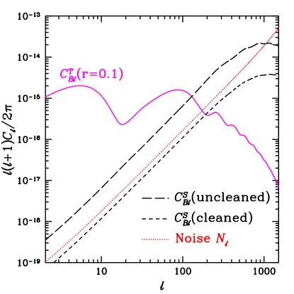
Figure 1: The tensor B mode power spectrum for $r=0.1$ and $\tau=0.17$ (solid) and the scalar B mode power spectrum (long dashes). The noise power spectrum for an experiment with $\Delta_{P}=3\sqrt{2}\mu K\cdot{\rm arcmin}$ and $\theta_{b}=3^{\prime}$ is shown with the dotted line. The short-dashed curve is the residual scalar B mode power spectrum after cleaning of the lensing contaminant by such an experiment.

IV Forecasting Detectability Limits

The cosmic microwave background (CMB) anisotropies are polarized at the last-scattering surface due to the quadrupolar temperature fluctuations seeded by the almost scale-invariant density fluctuations at horizon crossing. The different types of polarization are expected from the different sources of the quadrupolar temperature fluctuations: scalar, vector and tensor quadrupole anisotropy. The observable polarization patterns are separated into the gradient E-mode polarization having even parity and the curly B mode polarization having odd parity kamionkowski97 ; seljak97 .

The different sources of the quadrupolar temperature fluctuations contribute the polarization patterns in their own way. The scalar source leads to E-mode primarily, but the weak lensing effect due to the mass distribution along lines of sight between the observer and the last scattering leads to the transformed secondary B mode zaldarriaga98 of which amplitude is naturally smaller than the overall amplitude of the primary polarization. Vector perturbations have no growing modes in linear perturbation theory and thus are not expected to be significant in inflationary models for either E or B modes. The tensor source expected from the inflationary model has both E and B patterns in roughly equal magnitude kamionkowski97 ; seljak97 . Thus the B mode has the highest ratio of tensor-to-scalar fluctuation power and is what we consider.

We show the scalar power spectrum $C^{S}_{Bl}$ and the tensor power spectrum $C^{T}_{Bl}$ in Fig. 1 . With $r=0.1$, $C^{T}_{Bl}$ is greater than $C^{S}_{Bl}$ at $l<100$. The bump in $C^{T}_{Bl}$ at $l<20$ appears due to reionization. The amplitude is proportional to the square of the optical depth, $\tau$ zaldarriaga97a ; here we have set $\tau=0.17$. The detectability of the tensor B mode is enhanced by the reionization bump knox02 ; kaplinghat03b .

The primary temperature and polarization maps are distorted by the gradient of the projected lensing potential $\phi$. We can estimate $\phi$ from the 4-point function of the temperature and polarization fields okamoto02 . With $\phi$ estimated from the lensed maps, we can clean the lensed B mode. The cleaned and uncleaned $C^{S}_{Bl}$ are shown in Fig. 1. The residual lensing-induced B mode after cleaning is up to 10 times smaller than the uncleaned lensing-induced B mode. The minimum detectable limit of $r$ which we can achieve from the mass reconstruction is close to $2\times 10^{-5}$ which is 10 times better than with no cleaning knox02 ; kesden02 .

We use the the following cosmological parameters : $\Omega_{m}=0.34$, $\Omega_{b}=0.05$, $\Omega_{V}=0.66$, $h=0.66$, $\tau_{reion}=0.17$ and $\sigma_{8}=0.86$, and let $n_{T}$ and $r$ be free parameters. We use the high sensitive future CMB experiments with noise levels, $\Delta_{P}/\sqrt{2}=\Delta_{T}$ in the range $\Delta_{T}=1\mu K\cdot{\rm arcmin}$ to $15\mu K\cdot{\rm arcmin}$, angular resolution in the range $\theta_{b}=1.0^{\prime}$ to $30.0^{\prime}$ and full sky coverage ($f_{sky}=1$). Here $\Delta_{P}=\omega^{-1/2}$ and $\omega$ is the weight per solid angle for the $Q$ and $U$ linear polarization Stokes parameters.

The variance of B mode CMB power spectrum, $\Delta C^{B}_{l}$, is given by

$$\Delta C^{B}_{l}=\sqrt{2\over(2{l}+1)f_{sky}}\left(C_{l}^{B,T}+C_{l}^{B,S}+N_{l}\right),$$ (16)

where $C_{l}^{B,T}$ is the tensorial B mode and $C_{l}^{B,S}$ is the scalar B mode from lensing either before or after cleaning as in knox02 . $N_{l}$ is the experimental noise which is given by

$$N_{l}=\left({\pi\over 180\times 60}\,{\Delta_{P}\over{\rm T_{CMB}}}\right)^{2}{\rm e}^{l^{2}\theta_{b}^{2}/(8\ln 2)}.$$ (17)

Based on the Gaussianity of perturbations, we use the Fisher matrix analysis to estimate the detectability

$${\rm\bf F}_{pp^{\prime}}=\sum_{l}{\partial C^{B}_{l}\over\partial p}\left(\Delta C^{B}_{l}\right)^{-2}{\partial C^{B}_{l}\over\partial p^{\prime}},$$ (18)

where $p$ and $p^{\prime}$ enumerate the cosmological parameters we consider here. The diagonal elements of the ${\rm\bf F}_{pp^{\prime}}^{-1/2}$ are the 1-$\sigma$ errors for the parameters press92 .

The slow-roll parameter $\epsilon$ can be replaced by the measurable quantity $r$, the tensor to scalar ratio $T/S$, by using the fitting formula knox95 turner95 ,

$$\epsilon={1\over 14}\,\frac{1.04-0.82\Omega_{V}+2\Omega_{V}^{2}}{1.0-0.03\Omega_{V}-0.1\Omega_{V}^{2}}\,\,r.$$ (19)

The above fitting formula includes the non-negligible contribution to the quadrupole anisotropy from the late-time ISW effect.

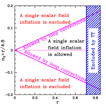
Figure 2: The solid lines bound the possible departures from the consistency equation for models with a single scalar field. The shaded area is excluded by observations of the temperature power spectrum spergel03 .

V results and discussion

Before turning to our detectability limits, we survey the $r$ vs. $n_{T}+2(A_{T})^{2}/(A_{S})^{2}$ plane. We first rewrite the consistency equation Eq. 14 with Eq. 19,

$$n_{T}+\frac{1}{4.8}r=-\frac{1}{4.8}\,r\,r_{l},$$ (20)

where $r_{l}$ is the loop corrections, $r_{l}\equiv\chi_{S}H^{2}/M^{2}$. The solid line in Fig. 2 is given by setting $r_{l}=1$, its maximum value. These are largest possible departure to the consistency equation. If the observed value of $n_{T}+r/4.8$ is outside the two solid lines in Fig. 2, the single scalar field slow-roll inflation model can be excluded. If the observed value of $n_{T}+r/4.8$ is inside the two solid lines and yet different from zero, we may have a chance to study physics at distances shorter than $1/M$. The current upper bound on $r$ from the temperature power spectrum is 0.71 bennett03 .

Our detectability limits are shown in Fig. 3. We fixed all parameters except $r$ and $n_{T}$ and calculated the Fisher matrix with $r$ varying from $10^{-5}$ to 0.71. We show the error on the combination $n_{T}+r/4.8$ since we are interested in testing the consistency equation, but $\sigma(n_{T})\simeq\sigma(n_{T}+r/4.8)$ since $\sigma(n_{T})>>\sigma(r)/4.8$. As expected, $\sigma(n_{T})$ decreases as $r$ increases and raises the signal level.

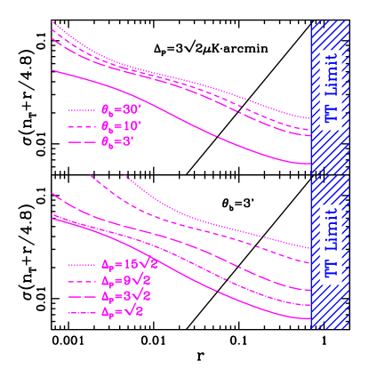
Figure 3: The error on $n_{T}+r/4.8$ as a function of $r$. The cosmic variance limit is the solid line in both panels. In the upper panel, we fix $\Delta_{P}=3\sqrt{2}\mu K\cdot{\rm arcmin}$ and vary the angular resolution: $\theta_{b}=1^{\prime}$ (long dash), $\theta_{b}=3^{\prime}$ (dash) and $\theta_{b}=5^{\prime}$ (dots). In the lower panel, we fix the angular resolution at $\theta_{b}=3^{\prime}$ and vary the weight per solid angle: $\Delta_{P}=\sqrt{2}\mu K\cdot{\rm arcmin}$ (dot-dashed), $\Delta_{P}=3\sqrt{2}\mu K\cdot{\rm arcmin}$ (long dash), $\Delta_{P}=9\sqrt{2}\mu K\cdot{\rm arcmin}$ (dash) and $\Delta_{P}=15\sqrt{2}\mu K\cdot{\rm arcmin}$ (dots). The shaded area is excluded by observations of the temperature power spectrum spergel03 .

From Fig. 3 we see that at $r<0.1$, any possible theoretical correction to the consistency equation for slow-roll single field models is beneath the detectability limit. Therefore, observing non-zero $n_{T}+r/4.8$ and $r<0.1$ will lead us to exclude the single slow-roll scalar field inflation scenario. At $r>0.1$, the loop correction terms begin to show up above the detectability limit. In this case, the broken consistency equation does not necessarily mean the failure of the single slow-roll scalar field inflation. The solid straight line indicates the maximal loop corrections with $r_{l}=1$. Only the broken consistency above this maximal loop corrections will mean the failure of the single slow-roll scalar field inflation at $r>0.1$.

We now consider all the next order corrections in Eq. 8. The term, $2(A_{T}^{4}/A_{S}^{4})=(r/4.8)\times(r/9.6)$, is always below the detectable limit with $r<0.71$. Also $2(A_{T}^{2}/A_{S}^{2})(1-n_{S})=r/4.8(1-n_{S})$ is well below the detectability limit in case of $n_{S}\sim 1$. Even if $n_{S}$ is much different from 1, we can control this term with the knowledge of $n_{S}$ from CMB scalar power spectrum. The future CMB experiment can determine the $n_{S}$ within $\sigma(n_{S})=0.0024$ kaplinghat03b . Thus it is obvious that no other correction terms is larger than the maximal loop correction terms, i.e. the solid straight line in Fig. 2 is the maximum theoretical bound which the correction terms in the consistency equation can reach.

In the upper panel of Fig. 3 we show the variation of the angular resolution with fixed $\Delta_{P}$. As the angular resolution decreases, the ability to clean out the contaminating scalar B mode diminishes and the detectability limit increases. We see that at $r>0.1$ cleaning can make up to a $\sim$50% decrease in the detectability limit. This is due to the improved measurement in the $l=20$ to $200$ range. At $r\simeq 0.01$ high angular resolution is less important, since the dominant source of information is now at $l<20$ which is unaffected by the scalar contamination.

In the lower panel of Fig. 3 we show the variation of $\Delta_{P}$ with fixed angular resolution. As $\Delta_{P}$ increases, the noise power becomes larger than the cleaned, and then even the uncleaned, scalar B mode power. This increased noise reduces the maximum observable tensor $l$ and adds significant noise all across the tensor B mode spectrum rise from $l\simeq 20$ to $l=100$. Thus there is a strong sensitivity to increases in the noise above our fiducial value.

The cosmological parameter with the most impact on the tensor spectrum is $\tau$. Although $\tau$ can make a big difference for the detectability limit of $r$ knox02 ; kaplinghat03b , it has little impact on the detectability limits for $n_{T}+r/4.8$. The $r$ limit is improved by increased $\tau$ since the ‘reionization bump’ at $l<20$ has $C_{l}\propto\tau^{2}$. In contrast, for acceptable values of $\tau$, and $r\mathrel{\mathchoice{\lower 3.6pt\vbox{\halign{$\mathsurround=0pt\displaystyle\hfil#\hfil$\cr>\crcr\sim\crcr}}}{\lower 3.6pt\vbox{\halign{$\mathsurround=0pt\textstyle\hfil#\hfil$\cr>\crcr\sim\crcr}}}{\lower 3.6pt\vbox{\halign{$\mathsurround=0pt\scriptstyle\hfil#\hfil$\cr>\crcr\sim\crcr}}}{\lower 3.6pt\vbox{\halign{$\mathsurround=0pt\scriptscriptstyle\hfil#\hfil$\cr>\crcr\sim\crcr}}}}0.01$, the error in $n_{T}+r/4.8$ is dominated by uncertainties in the tensor power spectrum at $l>20$. Here the only effect of reionization is a suppression of power by $exp(-2\tau)$.

Our analysis has ignored polarized emission from galactic and extragalactic sources. Multi–frequency observations can be used to clean out these signals based on their distinct spectral shapes. However, residual contamination is unavoidable and will also limit the ability of observations to study the consistency equation. As we learn more about polarized foreground emission, these will likely have a big impact on observing strategies and forecasted $n_{T}+r/4.8$ detectability limits below some value of $r$. Our forecasts should therefore be viewed as lower limits.

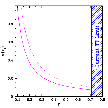
Figure 4: The detectable region of the loop corrections, $r_{l}$. The signature of the short distance physics is visible above the curve. The high resolution reference experiment here is $\Delta_{P}=3\sqrt{2}\mu K\cdot{\rm arcmin}$ $\&$ $\theta_{s}=3^{\prime}$. The dotted curve is the constraint from the uncleaned B mode. The solid curve is the constraint from the cleaned B mode.

We now turn our attention to the signature of the short distance physics; i.e., how well can we detect a non-zero value of $r_{l}\equiv\chi H^{2}/M^{2}$? Fig. 4 shows the narrow window for the detectability of $r_{l}$ which can be seen at $r>0.1$. As Kaloper et. al. pointed out, we cannot see the new physics at $r_{l}<0.1$, but some M theories with proper compactification give $r_{l}>0.1$ kaloper02 .

The window for probing the new physics is very narrow at $r>0.1$ and $r_{l}>0.1$. But it is a clean window from any next order correction in the slow roll parameters, since the next order corrections in Eq. 8 is beneath the detectability limit at this window. We conclude it is possible to probe physics at distances near $1/M$ as long as $r>0.1$ and $M$ is very close to $H$.

The dotted line in Fig. 4 is the forecasted constraint from the uncleaned B mode with the same experiment ($\Delta_{P}=3\sqrt{2}\mu K\cdot{\rm arcmin}$ $\&$ $\theta_{b}=3^{\prime}$). We get the solid line by cleaning the scalar B mode with the estimated lensing potential. If the reduced Planck mass is truly such a small amount, i.e. $r_{l}>0.1$, then even a small amount of improvement in $\sigma(r_{l})$ will be valuable. As we see in Fig. 4, the lensing potential reconstruction improves the detectability of $r_{l}$ by about 50%. If we can detect the tensor power spectrum at $r>0.1$, the uncleaned B mode can probe the tensor power spectrum well. But we will want the cleaned B mode to probe to even shorter distances.

Wands et al. wands02 have studied the consistency equation for two and more scalar fields. For two scalar fields there is a generalized consistency equation giving the tensor perturbation to scalar curvature perturbation ratio proportional to $n_{T}$ times an isocurvature correlation angle. For more than two fields this becomes an inequality, providing an upper bound on this tensor-to-scalar ratio. Thus observation of departure from this generalized consistency equation (by more than allowed by loop corrections) would rule out two–field models and an observed violation of the inequality would rule out all slow-roll models of inflation.

VI Conclusions

The tensor perturbation spectrum is a more direct probe of inflation than the scalar perturbation spectrum and may provide us with highly valuable information about the physics of inflation. We have quantified how well idealized versions of future experiments can probe the tensor perturbation spectrum and, in particular, test the inflationary consistency equation. Detectable departures may come from additional fields or short–distance corrections to the inflaton’s effective field theory. We have shown that for $r\mathrel{\mathchoice{\lower 3.6pt\vbox{\halign{$\mathsurround=0pt\displaystyle\hfil#\hfil$\cr>\crcr\sim\crcr}}}{\lower 3.6pt\vbox{\halign{$\mathsurround=0pt\textstyle\hfil#\hfil$\cr>\crcr\sim\crcr}}}{\lower 3.6pt\vbox{\halign{$\mathsurround=0pt\scriptstyle\hfil#\hfil$\cr>\crcr\sim\crcr}}}{\lower 3.6pt\vbox{\halign{$\mathsurround=0pt\scriptscriptstyle\hfil#\hfil$\cr>\crcr\sim\crcr}}}}0.01$, even though high resolution does not improve the detectability of $r$, high resolution does improve the detectability of departures from the consistency equation.

We thank Nemanja Kaloper for his feedback on a draft version of this manuscript and Andreas Albrecht, Eugene Lim and Sayan Basu for useful conversations. This work was supported in part by NASA NAG5-11098.

References

- (1) G. Hinshaw et al., ArXiv Astrophysics e-prints 2217 (2003).
- (2) T. J. Pearson et al., ArXiv Astrophysics e-prints 5388 (2002).
- (3) C. L. Kuo et al., ArXiv Astrophysics e-prints 12289 (2002).
- (4) A. Kogut et al., (2003), astro-ph/0302213.
- (5) W. Hu and M. White, Astrophys. J. 479, 568 (1997).
- (6) D. N. Spergel and M. Zaldarriaga, Physical Review Letters 79, 2180 (1997).
- (7) N. Kaloper, M. Kleban, A. Lawrence, and S. Shenker, Phys. Rev. D66, 123510 (2002).
- (8) A. Albrecht, N. Kaloper, and Y. Song, ArXiv High Energy Physics - Theory e-prints 11221 (2002).
- (9) N. Cornish, D. Spergel, and C. Bennett, ArXiv Astrophysics e-prints (2002).
- (10) A. H. Jaffe and D. C. Backer, Astrophys. J. 583, 616 (2003).
- (11) M. S. Turner, ArXiv Astrophysics e-prints 12281 (2002).
- (12) A. Albrecht and P. J. Steinhardt, Phys. Rev. Lett. 48, 1220 (1982).
- (13) J. E. Lidsey et al., Reviews of Modern Physics 69, 373 (1997).
- (14) A. R. Liddle, P. Parsons, and J. D. Barrow, Phys. Rev. D50, 7222 (1994).
- (15) E. D. Stewart and D. H. Lyth, Phys. Lett. B302, 171 (1993).
- (16) L. F. Abbott and M. B. Wise, Nucl. Phys. B244, 541 (1984).
- (17) A. R. Liddle and D. H. Lyth, Phys. Lett. B291, 391 (1992).
- (18) E. J. Copeland, E. W. Kolb, A. R. Liddle, and J. E. Lidsey, Phys. Rev. D49, 1840 (1994).
- (19) M. Kamionkowski, A. Kosowsky, and A. Stebbins, Phys. Rev. Lett. 78, 2058 (1997).
- (20) U. . Seljak and M. Zaldarriaga, Phys. Rev. Lett. 78, 2054 (1997).
- (21) M. Zaldarriaga, U. Seljak, and E. Bertschinger, Astrophys. J. 494, 491 (1998).
- (22) M. Zaldarriaga, Phys. Rev. D55, 1822 (1997).
- (23) L. Knox and Y.-S. Song, Phys. Rev. Lett. 89, 011303 (2002).
- (24) M. Kaplinghat, L. Knox, and Y. Song, ArXiv Astrophysics e-prints 3344 (2003).
- (25) T. Okamoto and W. Hu, Phys. Rev. D66, 63008 (2002).
- (26) M. Kesden, A. Cooray, and M. Kamionkowski, Phys. Rev. Lett. 89, 11304 (2002).
- (27) W. H. Press, W. T. Vetterling, S. A. Teukolsky, and B. P. Flannery, Numerical Recipes (Cambridge University Press, Cambridge, UK —c1992, ADDRESS, 1992).
- (28) L. Knox, Phys. Rev. D52, 4307 (1995).
- (29) M. S. Turner and M. White, Phys. Rev. D53, 6822 (1996).
- (30) D. N. Spergel et al., (2003), astro-ph/0302209.
- (31) C. L. Bennett et al., ArXiv Astrophysics e-prints 2207 (2003).
- (32) D. Wands, N. Bartolo, S. Matarrese, and A. Riotto, ArXiv Astrophysics e-prints 5253 (2002).
- (33) N. Turok, Phys. Rev. D54, 3686 (1996).
- (34) U. Seljak and M. Zaldarriaga, Astrophys. J. 469, 437 (1996).